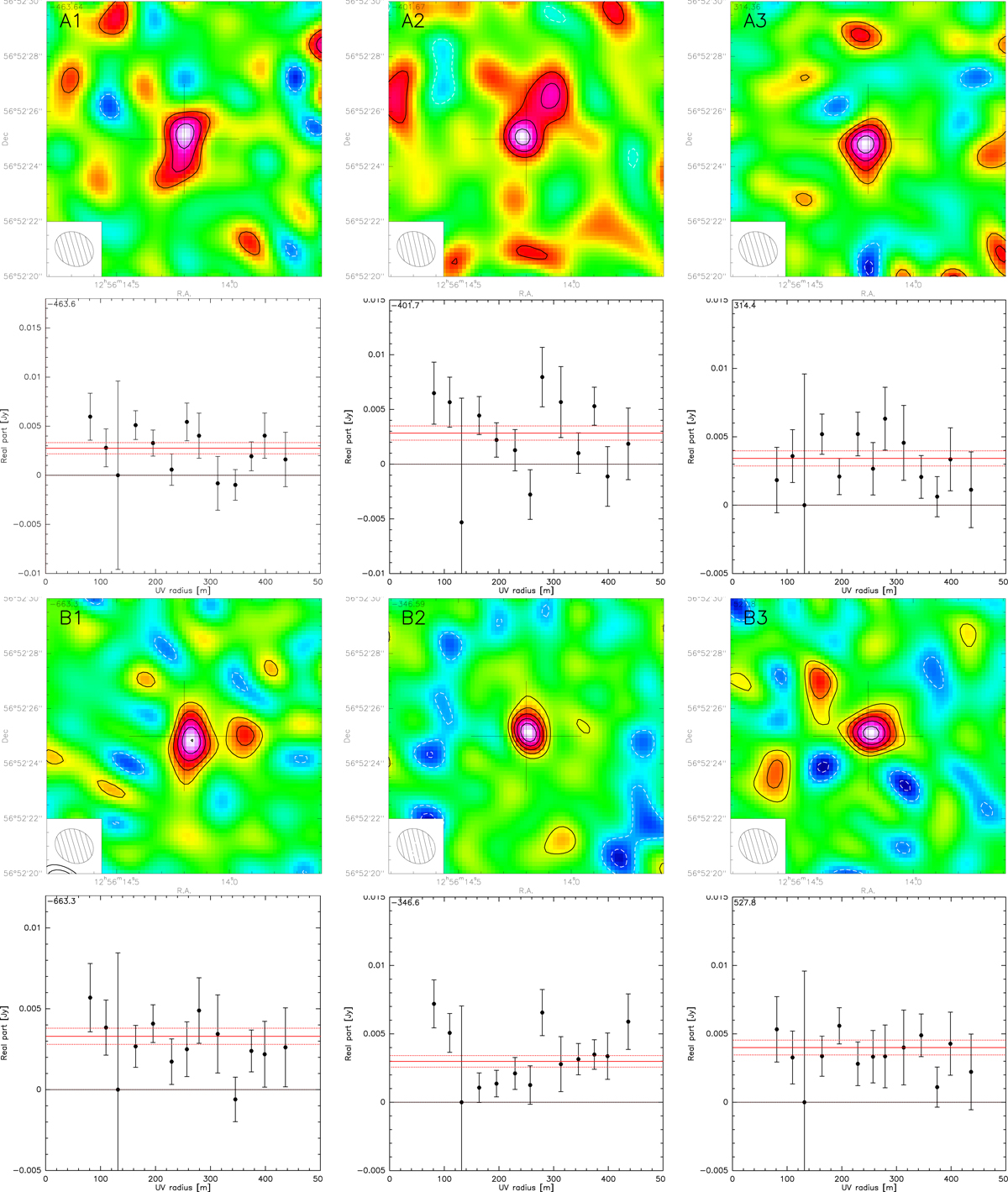
Interferometric maps and corresponding uv visibility plots of the HCN(1–0) clumps (top rows: A1, A2, and A3; bottom rows: B1, B2, and B3, see also labels in the top left corner of the maps). The maps show the continuum-subtracted emission integrated between v_c − 2σ_v <  v <  v_c + 2σ_v, where v_c and σ_v are the best-fit central velocity and velocity dispersion obtained from the spectral line fitting (Table 3). Each map is 10″ × 10″, and the synthesised beam is 1.45″ × 1.21″. Contours correspond to (−3σ, −2σ, 2σ, 3σ, 4σ, 5σ, and 6σ). Below each map we report the corresponding uv plot, binned in intervals of 30 m. The red solid and dashed lines represent the best-fit value and its associated uncertainty obtained using a point source model (Table 3).