Fig. 8
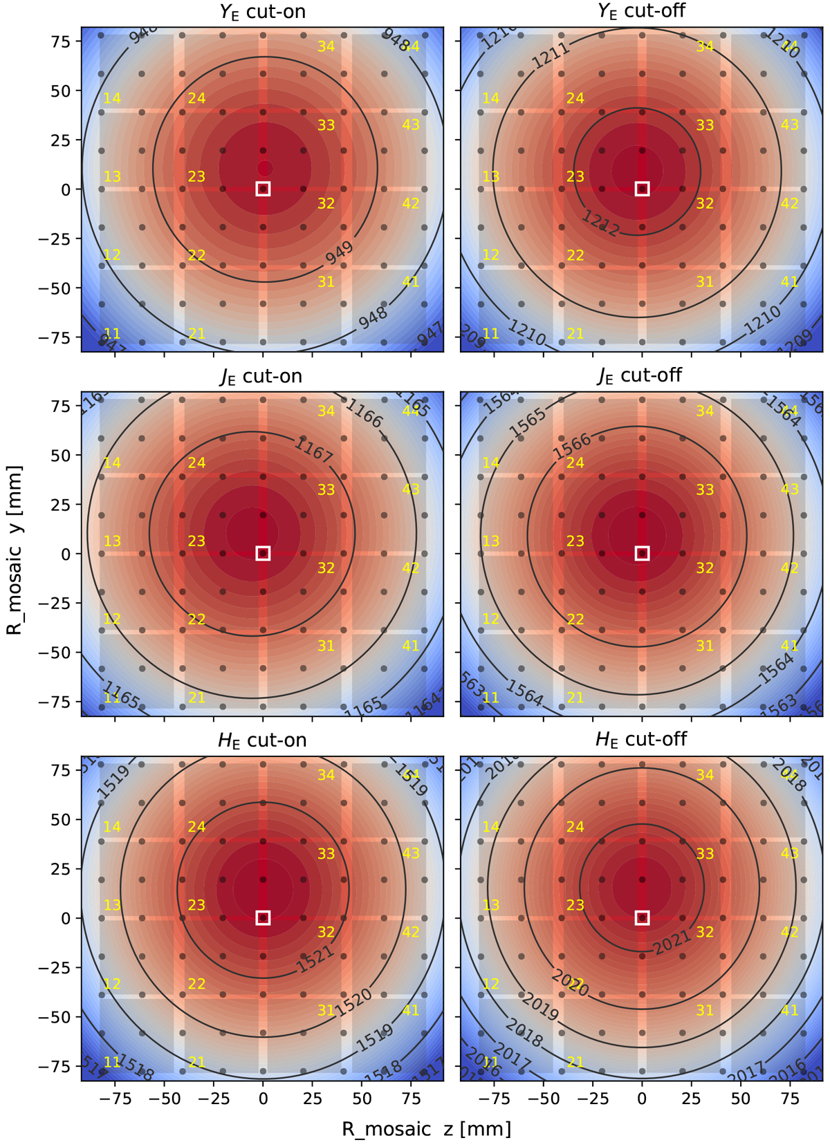
Download original image
Cut-on and cut-off wavelengths (in nm) as a function of FPA position, cold and in vacuum. The blueshift towards the field corners is evident. The black lines and coloured background show the polynomial fits introduced in Sect. 4.2; the fit parameters are listed in Table A.1, and the joint residuals are shown in Fig. 9. The fits are based on the 9×9 object positions (small dots) for which we inferred the AOI distribution on the filter surface using Zemax ray tracing. The shaded squares display the 16 NISP detectors, numbered in yellow from 11 to 44. The position of the number indicates the location of the (111) pixel of a detector. The published response curves (Sect. 7.2) were computed for the central dot marked with the white square. R_mosaic (z, y) is a physical coordinate system in the focal plane, to describe – among other factors – the detector positions.
Current usage metrics show cumulative count of Article Views (full-text article views including HTML views, PDF and ePub downloads, according to the available data) and Abstracts Views on Vision4Press platform.
Data correspond to usage on the plateform after 2015. The current usage metrics is available 48-96 hours after online publication and is updated daily on week days.
Initial download of the metrics may take a while.