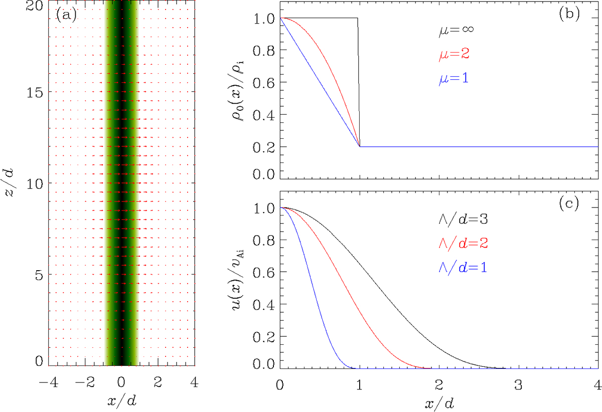
Equilibrium setup and initial exciters. (a) Representation of 2D initial boundary value problem (IBVP). The x − z distribution of the equilibrium density is shown by the filled contours, superimposed on which is the initial velocity field (the arrows). Axial fundamentals are ensured by the z dependence of the initial perturbation. (b) Transverse profiles of the equilibrium density ρ₀ as prescribed by Eq. (8). A number of steepness parameters μ are considered as labeled, whereas the density contrast is fixed at ρ_i/ρ_e = 5. (c) Transverse profiles of the initial perturbation u(x) as prescribed by Eq. (9). Labeled here are a number of values of Λ, which characterizes the spatial extent of the initial exciter.