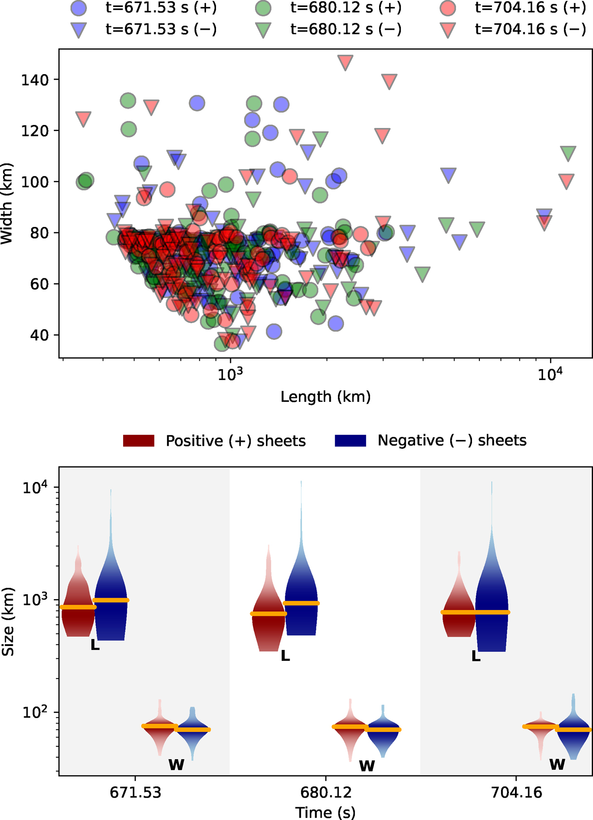
Fig. 7.
Download original image
Top: Scatter plot of all current sheets characterised in length being the longest dimension (horizontal) versus width (vertical) for three times: 73 clusters (positive) and 65 clusters (negative) for t = 671.53 s, 75 clusters (positive), and 62 clusters (negative) for t = 680.12 s, and 73 clusters (positive) and 70 clusters (negative) for t = 704.16 s (blue, green, and red, respectively). The ‘+’ refers to the positive current sheets while ‘−’ refers to the negative current sheets. Most of the current sheets are smaller ranging between 631–1388 km in length and of 61–78 km in width. The largest current sheet analysed by the algorithm in the simulation goes up to ∼11 355 km in length and around ∼116 km in width. Bottom: Statistical distribution of current sheet lengths and widths at the same times, shown as violin plots for positive (red) and negative (blue) current sheets. The width of each violin indicates the probability density estimated by kernel density estimation, while the solid orange horizontal lines mark the medians. The ‘L’ and ‘W’ labels denote distributions for length and width, respectively. Shading is used to visually separate the three time instances. These distributions reveal asymmetries between positive and negative sheets in both length and width, highlighting temporal evolution and polarity dependence in current sheet morphology of the simulation.
Current usage metrics show cumulative count of Article Views (full-text article views including HTML views, PDF and ePub downloads, according to the available data) and Abstracts Views on Vision4Press platform.
Data correspond to usage on the plateform after 2015. The current usage metrics is available 48-96 hours after online publication and is updated daily on week days.
Initial download of the metrics may take a while.