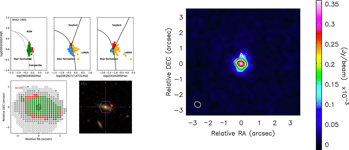
Fig. 1.
Download original image
Left panel: BPT diagram used to distinguish between ionisation by AGN (red spaxels), star formation (blue spaxels), composite (green spaxels), and LINER (yellow spaxels). The figure is adapted from Mezcua & Domínguez Sánchez (2020). Middle panel: The left figure shows the spatial distribution of the BPT-classified spaxels (colour-coded as in the top left panel). Empty squares mark the IFU coverage, grey squares mark those spaxels with S/N > 1. The radio contours at (10, 20, 40, 70) times the off-source RMS noise have been added on the image. The right figure is the SDSS composite image. The pink hexagon shows the IFU coverage. The figure is taken from Mezcua & Domínguez Sánchez (2020). Right panel: VLA radio image at 6 GHz. The colour bar indicates the flux of each pixel in Jy beam−1. Regions selected for Gaussian fitting are indicated by a letter. In the lower right corner is the clean beam (solid white or solid black line), which indicates the minimum beam size resolved in the observation and whose size is shown in Table 2. The radio contours have been added on the image.
Current usage metrics show cumulative count of Article Views (full-text article views including HTML views, PDF and ePub downloads, according to the available data) and Abstracts Views on Vision4Press platform.
Data correspond to usage on the plateform after 2015. The current usage metrics is available 48-96 hours after online publication and is updated daily on week days.
Initial download of the metrics may take a while.