Fig. 3.
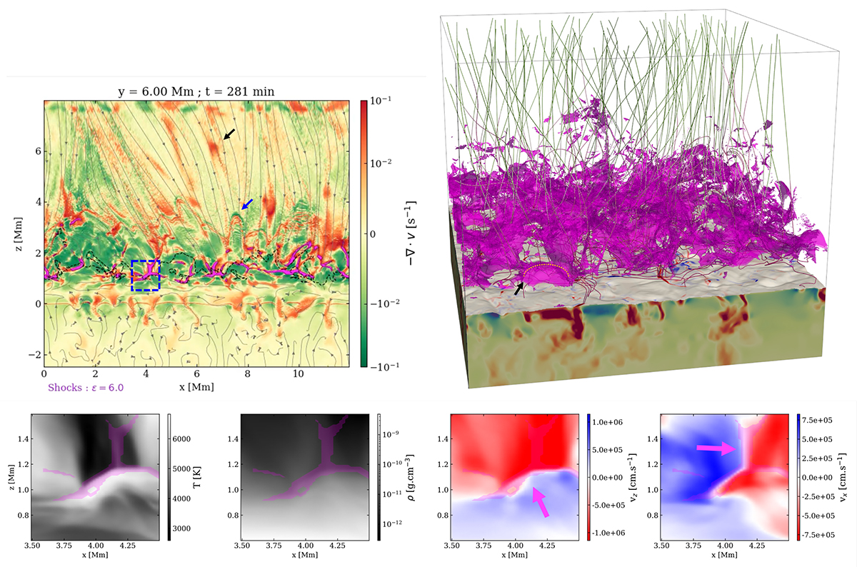
Download original image
Shock locations. Top-left: Compression frequency −∇ ⋅ v taken at Y = 6 Mm. Red and green areas denote compression and expansion, respectively, and magnetic polarity is illustrated along magnetic field lines (grey) with arrows. A zoom-in on the dashed blue square is provided in the bottom panels to highlight shock features (purple). The dark and blue arrows highlight particular compression locations due to wave propagation and rising over-density, respectively. The β = 1 surface is illustrated with a dashed black line. An animation covering 13 s (21 solar minutes) is available online. Top-right: 3D rendering of the shock fronts in the simulation domain at t = 274 min. This is similar to that in Fig. 1, but we do not colour magnetic field lines for the sake of clarity. Note that we use a dashed orange line, along with a dark arrow, to highlight the dome-like shape of a shock’s front. The locations of the magneto-acoustic shocks are highlighted in magenta in the two panels, which indicate large values of compression (−∇ ⋅ v > cs/(6.ds), see Eq. (1)). An animation covering 11 s (18 solar minutes) is available online. Bottom: Zoom-in on shock features, exhibiting from left to right the temperature, density, vertical and horizontal velocity, respectively. We note that the purple contours overlay the strong gradients of the different quantities. Purple arrows illustrate shock motions.
Current usage metrics show cumulative count of Article Views (full-text article views including HTML views, PDF and ePub downloads, according to the available data) and Abstracts Views on Vision4Press platform.
Data correspond to usage on the plateform after 2015. The current usage metrics is available 48-96 hours after online publication and is updated daily on week days.
Initial download of the metrics may take a while.