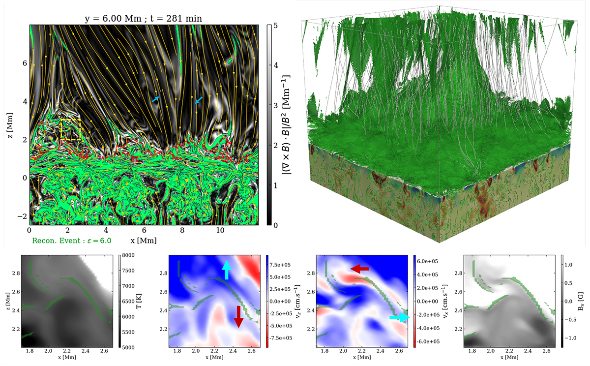
Fig. 4.
Download original image
CS location. Top-left: Normalised-parallel current |∇ × B ⋅ B|/B2 taken at y = 6 Mm. This quantity has the dimension of a spatial frequency, with white areas corresponding to high amplitudes. The magnetic polarity is illustrated along magnetic field lines (yellow) with arrows. A zoom-in on the dashed yellow square is provided in the bottom panels to highlight a CS feature. The β = 1 surface is illustrated with a dashed red line. The blue arrows are used to highlight particular locations of weaker and broader current layers, not labelled as CSs following Eq. (3), likely due to wave propagation, magnetic field braiding, and phase mixing. The β = 1 surface is illustrated with a dashed red line. An animation covering 12 s (20 solar minutes) is available online. Top-right: 3D rendering of CSs in the simulation domain at t = 224 min. The locations of CSs are highlighted in green in the two panels, which indicate large values of the normalised-parallel current (|(∇ × B)⋅B|/B2 > 1/(6.ds); see Eq. (3)). Bottom: Zoom-in on CS features, exhibiting from left to right the temperature, vertical velocity, horizontal velocity, and magnetic field component, respectively. We note that the green contours overlay the strong gradients in the Bx and bipolar velocity patterns. Cyan and dark red arrows illustrate these motions.
Current usage metrics show cumulative count of Article Views (full-text article views including HTML views, PDF and ePub downloads, according to the available data) and Abstracts Views on Vision4Press platform.
Data correspond to usage on the plateform after 2015. The current usage metrics is available 48-96 hours after online publication and is updated daily on week days.
Initial download of the metrics may take a while.