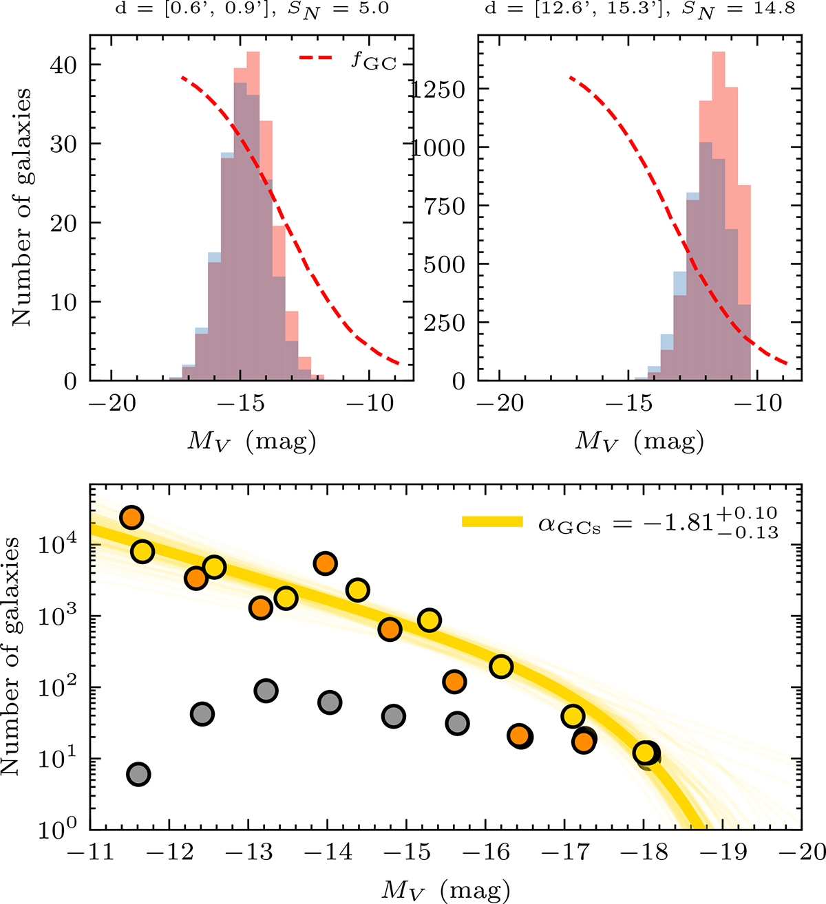
Fig. G.1.
Download original image
Constraint to the faint end of the past LF following the method described in Appendix G. Top panels: examples of two radial bins and their associated primordial LFs according to the measured SN. In each panel, the blue histogram shows the Gaussian LF for the associated value of SN, with dispersion σ = 0.9 mag and normalised to the luminosity inside the bin. The red histogram shows the skewed LF obtained after dividing the non-normalised Gaussian LF by the GC occupation fraction profile (red dashed line), and then normalising to the bin luminosity. Bottom: Faint-end constraint to the past LF considering the contribution from all annuli (gold), compared to the present-day LF (grey) and the past LF obtained with the simplified method (orange).
Current usage metrics show cumulative count of Article Views (full-text article views including HTML views, PDF and ePub downloads, according to the available data) and Abstracts Views on Vision4Press platform.
Data correspond to usage on the plateform after 2015. The current usage metrics is available 48-96 hours after online publication and is updated daily on week days.
Initial download of the metrics may take a while.