| Issue |
A&A
Volume 709, May 2026
|
|
|---|---|---|
| Article Number | A129 | |
| Number of page(s) | 11 | |
| Section | Numerical methods and codes | |
| DOI | https://doi.org/10.1051/0004-6361/202558275 | |
| Published online | 08 May 2026 | |
Accurate spectroscopic redshift estimation using nonnegative matrix factorization: Application to MUSE spectra
1
Université Lyon 1, ENS de Lyon, CNRS, CRAL, UMR 5574,
Saint-Genis-Laval,
France
2
Leibniz-Institut für Astrophysik Potsdam (AIP),
An der Sternwarte 16,
14482
Potsdam,
Germany
3
Instituto de Astrofísica e Ciências do Espaço, Universidade do Porto, CAUP,
Rua das Estrelas,
4150-762
Porto,
Portugal
4
Departamento de Física e Astronomia, Faculdade de Ciências, Universidade do Porto,
Rua do Campo Alegre 687,
4169-007
Porto,
Portugal
5
Institut für Physik und Astronomie, Universität Potsdam,
Karl-Liebknecht-Str. 24/25,
14476
Golm,
Germany
6
National Astronomical Observatory of Japan,
2-21-1 Osawa, Mitaka,
Tokyo
181-8588,
Japan
★ Corresponding author: This email address is being protected from spambots. You need JavaScript enabled to view it.
Received:
26
November
2025
Accepted:
4
March
2026
Abstract
Accurate and automated galaxy redshift determinations are essential for maximizing the scientific return of spectroscopic surveys. In this paper, we propose a data-driven method to address this challenge. The method first learns a rest-frame representation of galaxy spectra using nonnegative matrix factorization (NMF). The method then reconstructs new spectra using this representation at different trial redshifts and identifies the correct redshift by selecting the one that minimizes the reconstruction error. We applied our method to galaxy spectra from the Multi Unit Spectroscopic Explorer (MUSE), covering redshifts from 0 to 6.7. Our method achieves an overall success rate of 93.7%. We demonstrate two applications: (i) the separation between true and false sources and (ii) the detection of blended sources from one-dimensional spectra. Our results demonstrate that NMF-based representations provide a powerful and physically motivated framework for redshift estimation in current and future large spectroscopic surveys.
Key words: instrumentation: spectrographs / methods: data analysis / techniques: imaging spectroscopy / techniques: spectroscopic / surveys / galaxies: general
© The Authors 2026
 Open Access article, published by EDP Sciences, under the terms of the Creative Commons Attribution License (https://creativecommons.org/licenses/by/4.0), which permits unrestricted use, distribution, and reproduction in any medium, provided the original work is properly cited.
This article is published in open access under the Subscribe to Open model. This email address is being protected from spambots. You need JavaScript enabled to view it. to support open access publication.
1 Introduction
All-sky Multi-Object Spectroscopic (MOS) surveys such as the Sloan Digital Sky Survey (SDSS York et al. 2000) and its upgrades (BOSS, eBOSS) have ushered astronomy into the big-data era, producing millions of spectra for objects down to 18–19 mag. MOS surveys on four meter-class telescopes, including Dark Energy Spectroscopic Instrument (DESI DESI Collaboration 2022), 4-Meter Multi-Object Spectroscopic Telescope (4MOST de Jong et al. 2019), and WHT Enhanced Area Velocity Explorer (WEAVE Dalton et al. 2012), now deliver tens of millions of spectra reaching ∼ 22 magnitude. Installed on a larger telescope, the Multi-Object Optical and Near-infrared Spectrograph (MOONS Cirasuolo et al. 2020) at the VLT will extend this capability into the near-infrared (NIR). To maximize the scientific outcome of these large data surveys, strategies to perform fast, efficient, and accurate automated object classification and redshift identification have been developed.
State-of-the-art tools for automated galaxy redshift estimation rely on spectral template fitting, in which a basis of galaxy spectra is first constructed and subsequently used to match observations across trial redshifts. These tools adopt different techniques and strategies to build a set of representative templates of the galaxy population. For example, Bolton et al. (2012) used a principal component analysis (PCA) procedure that accounts for measurement errors and missing data to learn a rest-frame representation of SDSS galaxies. Similarly, AUTOZ (Baldry et al. 2014), MARZ (Hinton et al. 2016; Inami et al. 2017), and xPCA (Krogager, in prep) employ cross-correlation with a set of data-driven templates obtained with PCA, where the stellar continuum is subtracted. Redrock (Anand et al. 2024) developed for the DESI pipeline uses a set of synthetic archetype galaxy templates that were obtained from stellar population synthesis and models of emission line fluxes. Deep learning approaches have also been explored to derive rest-frame representations. For instance, Zhong et al. (2025, 4MOST) trained an encoder network GaSNet-III to learn a rest-frame representation of SDSS galaxy spectra and use it for redshift predictions, achieving a competitive level of accuracy. Other deep learning models that do not rely on a rest-frame representation have also been explored. Zhong et al. (2025) trained a U-net network to transform spectra from the observed to the rest frame directly. Another example of such approaches is M-TOPnet (Ginolfi et al. 2025, MOONS). This network was trained through a multitask learning framework to simultaneously predict the redshift probability density function, stellar mass, star formation rate, and emission-line locations from the continuum-subtracted spectrum and a condensed continuum vector. All of these tools have demonstrated high speed, accuracy, and robustness within their respective MOS survey contexts.
While MOS surveys cover relatively bright preselected objects from imaging surveys, integral field spectroscopy (IFS) instruments, such as the Multi Unit Spectroscopic Explorer (MUSE Bacon et al. 2010), provide spectra for all the objects in the field; namely, without preselections, down to magnitudes of 28 and beyond (Bacon et al. 2017, 2023). At the same time, MUSE poses specific challenges due to its wavelength coverage resulting in objects detected over a wide redshift range (z = 0–6.7), which can lead to emission line confusion, especially between [O II] λλ3727, 3729 Å at z < 1.5 and Lyα λ1216 Å at z > 2.8. Thanks to its exquisite sensitivity, MUSE can efficiently find emission line objects without any continuum. As a result, the task of source detection and redshift identification in deep fields needs to be performed twice (Bacon et al. 2023): once on continuum-detected objects and once on emission line-detected objects. Currently, no existing tool can perform well on both types without visual inspections and validation. In addition, in the “redshift desert” at 1.5 < z < 2.8, galaxies lack strong spectral emission features, making redshift determination heavily dependent on continuum shape. These challenges call for new approaches capable of handling both continuum and emission line-dominated spectra across the full MUSE redshift range.
We present a method for automated galaxy redshift prediction, enabled by the availability of approximately 10 000 MUSE spectra with redshift labels. Our approach is based on non-negative matrix factorization (NMF), which learns a low-rank, additive, and nonnegative representation of galaxy spectra. By enforcing nonnegativity, NMF provides a parts-based and more interpretable representation compared to other techniques such as PCA. Moreover, NMF has been successfully applied in astrophysics to construct empirical spectral templates (Blanton & Roweis 2007) and to identify fundamental mid-infrared (MIR) components of galaxy spectra from Spitzer/IRS (Hurley et al. 2013), demonstrating its effectiveness. The method finds the best redshift solution by nonnegatively projecting a spectrum onto this representation for a range of trial redshifts and then selecting the projection with the lowest reconstruction error. We have applied our method to an independent test set and demonstrate its robustness in this work.
This paper is organized as follows. In Sect. 2, we describe the data selection and preprocessing procedures. Sect. 3 presents the application of NMF to MUSE galaxy spectra and the general methodology underlying our redshift prediction framework. In Sect. 4, we report the test results and present two applications of the method: (i) false and true source separation; and (ii) spectral deblending. Finally, we discuss our results in Sect. 5 and our conclusions in Sect. 6.
2 Data
In this work, we used a collection of galaxy spectra taken from five MUSE Guaranteed Time Observations (GTO) surveys: (i) MUSE Hubble Ultra-Deep Field (HUDF) surveys (Bacon et al. 2023, PI: R. Bacon); (ii) MusE GAs FLOw and Wind [MEGAFLOW] survey (Bouché et al. 2025, PI: N. Bouché); (iii) MUSCATEL survey (Urrutia, in prep; PI: L. Wisotzki); and (iv) MUSE-WIDE DR1 survey (Urrutia et al. 2019, PI: L. Wisotzki) and MUSE gAlaxy Groups in COSMOS (MAGIC) survey (Epinat et al. 2024, PI: T. Contini).
The combination of these surveys provides a representative and diverse sample of galaxy spectra for learning and analysis. It includes galaxies of different types and spectral characteristics, from continuum-dominated systems to strong emission- and absorption-line galaxies, spanning a wide range of redshifts and magnitudes. The mixture of deep and shallow fields observed under different conditions provides spectra with varying signal-to-noise ratios (S/Ns), enabling us to evaluate the robustness of our methods under realistic observational conditions. Table 1 summarizes some of the key characteristics of each survey.
From these surveys, we selected spectra of galaxies based on two criteria. First, we required a secure redshift by selecting galaxies with a redshift confidence score (ZCONF) of 1 or higher1. Second, we visually inspected the spectra to exclude most of the bright blended spectra “blends” (overlap between multiple sources).
Our selection yielded a sample of 9252 spectra. In Fig. 1, we summarize the main properties of the sample, showing the distributions of redshift, ZCONF, continuum S/N (S/Ncont), and S/N of the lines (S/Nlines). We computed S/Ncont as the median S/N of the stellar continuum in the observed-frame 7650–7850 Å window, chosen for its location within the region of highest MUSE throughput. In a given spectrum, we computed S/Nlines as the quadrature sum of the S/N values of all the detected emission and absorption lines with detection significances exceeding 3σ. The stellar continuum fit and line measurements were performed with the pyPlatefit package (Bacon et al. 2023), specifically developed for MUSE spectra. The preprocessing steps specific to our method are described in the following section.
Summary of the MUSE surveys used in this work.
3 Methods
3.1 Nonnegative matrix factorization
Nonnegative matrix factorization is a machine learning technique for dimensionality reduction (Lee & Seung 1999). Given a data matrix, X, NMF learns a low-dimensional representation by approximating X as the product of two nonnegative, low-rank matrices, W and H,
 (1)
(1)
In the specific case of galaxy spectra arranged row-wise in X (see, Fig. 2), NMF reconstructs each spectrum in X as a positive linear combination of k basis vectors in H with coefficients placed in the corresponding row of W. The number of basis vectors is directly controlled by the rank k; its value is free and must be fine-tuned (as detailed in Sect. 3.5).
The prevalent algorithm to solve Eq. (1) is described in the seminal work of Lee & Seung (1999). In our case, we adopt the more sophisticated “nearly NMF” algorithm developed by Green & Bailey (2024) specifically for astronomical spectra. nearly NMF extends Lee & Seung (1999) and Zhu (2016) algorithms to account for heteroscedastic uncertainties and missing values. It also considers negative values in X, known to cause offsets in basis vectors if zero-clipped (Green & Bailey 2024). Briefly, they considered the following optimization problem,
 (2)
(2)
where matrix Y2 holds the minimum shift to make each entry in X nonnegative. F = 1/σ2 is the inverse-variance matrix associated with X, a zero weight is assigned to missing entries. To minimize this objective, they derived multiplicative iterative update rules for W and H matrices that guarantee convergence to a local minimum,
![Mathematical equation: $\matrix{{H = H \odot {{{{\left[ {{W^T}(V \odot X)} \right]}^ + }} \over {{W^T}(V \odot (WH)) + {{\left[ {{W^T}(V \odot X)} \right]}^ - }}},} \hfill \cr {W = W \odot {{{{\left[ {(V \odot X){H^T}} \right]}^ + }} \over {(V \odot (WH)){H^T} + {{\left[ {(V \odot X){H^T}} \right]}^ - }}},} \hfill \cr }$](/articles/aa/full_html/2026/05/aa58275-25/aa58275-25-eq3.png) (3)
(3)
where ⊙ is the element-wise product. Operation [ ]+ applied on a matrix results in a matrix of the same shape, in which all negative values are zeroed. On the other hand, [ ]− cancels out the positive values and takes the absolute value of negative values.
Next, we describe how we construct the matrix X and the related processing steps. We then explain (in Sect. 3.3) how we can predict redshift using NMF learned basis vectors and present several metrics used to validate the predictions (in Sect. 3.4). Finally, we present the rank selection and validation methods in Sect. 3.5.
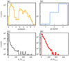 |
Fig. 1 Main statistical properties of the selected MUSE galaxy sample. Distributions of (a) redshift; (b) redshift confidence score (ZCONF)’ (c) stellar continuum S/N (S/Ncont), and (d) emission and absorption lines collective S/N (S/Nlines). |
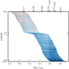 |
Fig. 2 MUSE galaxy spectra matrix in the rest frame. This matrix shows selected MUSE galaxy spectra, prepared for NMF decomposition. Spectra are sorted by increasing redshift (from bottom to top) and transformed to their rest frame. Key redshifts are shown on the y-axis and important spectral lines are indicated on top of the figure. The color of each pixel encodes flux density, scaled using a 95% z-scale to enhance the visibility of emission lines. Bluer colors represent higher flux densities; white pixels denote missing or unobserved data. |
3.2 Data transformation
The rest frame is more effective for learning a representation of galaxy spectra with NMF, as spectral features align consistently at fixed wavelengths, enabling their learning. Consequently, we transformed our MUSE galaxy spectra sample to the rest frame, with the following steps:
1. We defined a common rest-wavelength grid, Γ, in logarithmic space. This grid spans the range 2.77 ≤ log10 λ ≤ 3.97, with a uniform logarithmic spacing of ∆ log10 λ = 2.215525 × 10⁻⁵. The lower end of the grid corresponds to the bluest MUSE wavelength (λobs,min = 4600 Å), and transformed into the rest frame assuming a maximum redshift of zmax = 6.7. The upper end of the grid is given by the reddest MUSE wavelength (λobs,max = 9350 Å) at redshift zero. We derived the grid’s spacing, ∆ log10 λ, from an equivalent reference linear grid. This linear grid spans the same spectral range and has a step size, ∆λref, determined by the maximally squeezed MUSE spectral sampling (δλ) in the rest frame,

When this linear grid is transformed directly into logarithmic space, it produces nonuniform logarithmic spacings. ∆ log10 λ is then taken as the mean of these resulting logarithmic spacings to define a constant. These choices resulted in a 53 918-dimensional grid.
2. We express flux densities fλ in terms of the logarithmic rest wavelengths,
 (4)
(4)
where λrest, λobs are, respectively, the rest and observed wavelengths and z is the redshift.
3. For each spectrum, we linearly interpolated the pairs (fλ(log10 λrest), log10 λrest) to the rest-frame wavelength grid, Γ, and extrapolated with zeros in unobserved regions of Γ. Variances underwent the same transformations, except for the extrapolation part, where we assigned a large number instead of zero. Figure 2 shows the result of the rest-frame transformation of our sample of galaxy spectra.
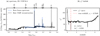 |
Fig. 3 Illustration of redshift prediction with NMF basis vectors. (a) Rest-frame spectrum of the UDF10-4 source at redshift 0.7649 in blue. This galaxy exhibits stellar continuum, strong [O II], Hβ, and [O III] spectral emission lines (their locations are indicated on top of the figure); the best NMF reconstruction is plotted in black. (b) Corresponding χ2 curve, the minimum happens at the true redshift (vertical red dashed line), hence, successfully predicting the correct redshift. The second minimum in the χ2 curve at z ∼ 4.4 corresponds to a solution in which [O II] gets mistaken to be Lya. The values of the ∆χ2 and R metrics are also reported in (b); their values indicate a significant minimum and a very robust redshift prediction. |
3.3 Estimating redshift using NMF basis vectors
Our method posits that the correct rest-frame of NMF basis vectors, aligned with the true redshift zt, achieves the best representation for a given observed galaxy spectrum. Conversely, an incorrect rest-frame will result in a poorer representation. For instance, consider a spectrum exhibiting nebular emission lines such as [O II], Hβ, and strong and weak [O III]. Only the correct rest-frame allows for a simultaneous and accurate reconstruction of all these features. In contrast, an incorrect rest frame could still reconstruct individual emission lines but will fail to model all of them collectively, as they are intrinsically absent.
Following this principle, to determine the redshift of an observed spectrum, fλ, obs, we tested all redshifts in the 0 ≤ z ≤ 6.7 range with a step of 0.0005. For each test redshift, ztest, we proceeded as follows:
- (a)
We de-redshifted the spectrum to its rest frame, assuming ztest, following the steps detailed in Sect. 3.2, we note the de-redshifted spectrum, fλ, test.
- (b)
We reconstructed fλ, test using NMF basis vectors,
 (5)
where the vector, ω, contains decomposition coefficients. Eq. (5) is solved using a nonnegative least squares (Bro & De Jong 1997), ensuring that the coefficients are nonnegative as in NMF.
(5)
where the vector, ω, contains decomposition coefficients. Eq. (5) is solved using a nonnegative least squares (Bro & De Jong 1997), ensuring that the coefficients are nonnegative as in NMF. - (c)
We assessed the reconstruction quality at ztest by computing the corresponding χ2 goodness-of-fit statistic,
 (6)
where σλ, test, is the corresponding standard deviations vector of fλ, test and L is the spectral dimension.
(6)
where σλ, test, is the corresponding standard deviations vector of fλ, test and L is the spectral dimension.
Testing all redshifts results in a χ2(z) curve. The minimum of this curve,  , then gives the predicted redshift, zp. Moreover, we characterized this minimum with a ∆χ2 value and a robustness score (see next subsection for definitions). We illustrate our method for a galaxy spectrum taken from the MXDF survey in Fig. 3a and we show the corresponding χ2 curve in Fig. 3b.
3.4 Evaluation metrics
To evaluate a redshift prediction, we used the following quantities from the χ2(z) curve,
(a) Redshift significance score3:
 (7)
(7)
where  denotes the minimum of the χ2 curve and Q1(χ2) its first quartile. The first quartile provides a robust estimate of the typical χ2 away from the minimum (baseline of the χ2 curve).
Thus, the quantity ∆χ2 measures how much the minimum deviates from the baseline of the χ2 curve, with higher values reflecting more significant minima.
(b) Redshift robustness score3:
 (8)
(8)
min(1)(χ2) and min(2)(χ2) denote the first and second minima of the χ2 curve, respectively. The quantity σQ1(χ2) is the standard deviation of all χ2 values less than or equal to the first quartile. It provides an estimate of the intrinsic dispersion of points lying on or below the χ2 curve baseline. Normalizing the separation between the first and second minima by σQ1(χ2) measures its significance relative to the typical fluctuations of the χ2 curve, while being insensitive to high-χ2 fluctuations. As the two minima approach each other, the score tends toward zero, indicating confusion between two redshift solutions.
To test our method on a set of spectra with known redshifts, we used the following metrics from the predicted and true redshifts:
(a) Relative error:
 (9)
(9)
where zp is the predicted redshift and zt the true redshift.
(b) The good fraction (GF):
This is the ratio of the number of good redshift predictions, Ngood, to the total number of predictions, Ntotal. A redshift prediction is good when its error is ∆z = |zp − zt| < tMUSE (1 + zt), where tMUSE is the adopted error-tolerance threshold. In this work, we fixed tMUSE at 0.005, which corresponds to a value ten times the step size in the trial redshifts. Thus, we have
 (10)
(10)
(c) Mean absolute error with outlier rejection:
 (11)
(11)
The redshift predictions with a relative error five times larger than the median absolute deviation (MAD) were rejected, where the MAD is defined as

where δz is the vector of redshift relative errors.
3.5 Rank selection and validation of the method
The factorization rank, k, sets the number of basis vectors in the NMF decomposition and therefore controls the level of detail the model can represent. If k is too large, the model may adjust to noise; whereas if it is too small, it may fail to capture important spectral features. In both cases, the resulting basis vectors generalize poorly, making careful rank selection essential.
In this work, we propose a rank selection strategy based on the performance in the redshift prediction task. We employed a K-fold cross-validation scheme (Kohavi 1995), where the data are partitioned into K folds, with K-1 folds used to learn basis vectors under various rank hypotheses, and the performance is evaluated on the withheld fold. This process is repeated until each of the K folds has served as the testing set once. The best rank is then taken to be the one that provides the best performance across all testing folds.
Given that our spectra matrix, X, is large (9252 × 53 918), we chose K = 5, which is a good trade-off between computational speed, bias, and variance. We used the GF and MAE to quantify redshift prediction performance on the test folds. The results of this exercise are reported in Fig. 4.
We observed an improvement in the GF up to a rank of 10, beyond which it plateaus. In contrast, the MAE (with outlier rejection) increases steadily with rank, indicating that while a larger rank does not degrade the GF, it leads to less precise redshift estimates for nonoutliers. Based on these observations, we fixed the rank at 10 for the remainder of this work, as it gives the highest success rate and more precise redshift estimates compared to higher ranks.
To conclude this section, we present in Fig. 5, the basis vectors obtained from a rank–10 NMF decomposition, applied to 80% of our sample. The basis vectors capture a broad range of spectral features, including prominent emission and absorption lines such as Lyα, [O II], CaKH, Hβ, [O III], and Hα, with varying relative line ratios across components. In addition, they encode distinct stellar continuum characteristics; for example, vector 10 is associated with red, evolved galaxy populations. Vector 1 shows a blue continuum with a clear UV spectral slope indicative of star-forming galaxies. We further note that several emission lines, in particular [O II] (see panel b), do not always coincide with their nominal rest-frame wavelengths (indicated by the vertical gray lines). Instead, the line center appears blue-shifted in vectors 1 and 9, redshifted in vector 5, and consistent with the rest frame in the remaining vectors. A similar behavior is observed for Lyα, which additionally exhibits a blue bump in some components. These variations indicate that the NMF basis naturally captures kinematic and radiative transfer effects present in the galaxy spectra. A schematic overview of the main steps of our method is provided in Fig. 6.
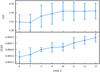 |
Fig. 4 NMF rank selection. Top and bottom panels: Mean GF and mean MAE with outlier rejections across the test folds, respectively, for ranks of 6–13. Corresponding standard deviations are shown as error bars. Both metrics are reported for spectra with ZCONF values of 2 and 3. |
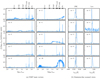 |
Fig. 5 NMF-learned basis vectors. Panel a shows the basis vectors obtained from a sequential rank–10 NMF decomposition applied to 80% of the sample. The index n labels each basis vector. The names and rest-frame wavelengths of prominent spectral emission and absorption lines are indicated in the upper panels. Panel b presents zoomed-in views of the [O II] and Lyα emission lines, shown in the first and second columns, respectively. In each zoom-in, the line’s peak flux is normalized to one, the line rest wavelength is shown with a vertical dashed gray line, and the corresponding basis vector is indicated. |
4 Results
4.1 Performance results
We evaluated the performance of our method using the first fold of the K-fold cross-validation setup. Rank-10 NMF basis vectors were derived from the learning subset and performance was assessed on the testing subset, ensuring that no spectral data from the test set influenced the learning process. This evaluation focused exclusively on 1454 spectra with a ZCONF ≥ 2.
Figure 7 shows the scatter of the predicted redshift (zp) against the true redshift (zt). Our method successfully recovers the redshift for 1363 spectra (points on the diagonal), while 91 spectra have bad predictions (off-diagonal points), yielding an overall GF of 93.7%. An inspection of the failures reveals three main causes: (1) spectra with poor flat-fielding, characterized by distorted continua at the blue and red ends; (2) spectra with a large fraction of negative flux values (negative median flux); and (3) confusion between the [O II] doublet and Lyα, especially in spectra lacking a stellar continuum and/or with broadened [O II] profiles due to galaxy kinematics. The latter confusion appears as a secondary diagonal above the main one in the scatter plot.
Figure 8 presents the relative error, δz, as a function of the significance score, ∆χ2, (panel a) and the Robustness metric R (panel b). We observe that almost all failed predictions correspond to ∆χ2 < 0.05 and R < 3. Moreover, we note that the R distribution peaks at 5 and failed predictions cluster on the left tail of this distribution; a cut in R can therefore be used to secure redshifts (pure selection). Cases with R > 3, but incorrect predictions, are associated with spectra dominated by negative flux values.
The three panels in Fig. 9 present the average GF as a function of redshift, continuum S/N, and S/N of the lines. Overall, the GF remains above 90% across most redshift bins, with notable declines in the redshift desert (z ∼ 2 and z ∼ 2.8) and at very high redshift (z ≥ 6). In the redshift desert, the reduced performance is due to the lack of strong spectral features in the spectra. At the highest redshifts, the GF has large uncertainties due to the small number of objects in these bins. When examined as a function of continuum S/N, the GF is largely stable and remains above 90% for nearly all bins, exhibiting only mild fluctuations at low S/N. A modest performance improvement is observed toward higher continuum S/N values, although the dependence is comparatively weak. In contrast, the strongest dependence is seen as a function of the lines’ S/N. The GF is very low for S/Nlines ≲ 7, rises steadily with increasing S/N, and approaches unity at S/Nlines ∼ 13, beyond which it plateaus. This trend indicates that the number of emission and absorption lines and their S/N values are the dominant factors governing the GF.
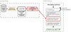 |
Fig. 6 Redshift prediction workflow using a rest-frame representation learned with nearly NMF. |
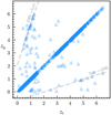 |
Fig. 7 Scatter plot of the predicted redshift (zp) against true redshift (zt) for the test set. Dashed gray lines mark predicted redshifts for [O II] sources misidentified as Lyα sources and vice versa. |
4.2 Performance with varying depth
Increasing survey depth improves data quality by reducing noise and enables the detection of faint objects. To investigate the impact of exposure time on our method, we applied it to four samples of spectra with different exposure times: MXDF (∼ 140 hours), UDF10 (∼ 30 hours), MEGAFLOW medium fields (∼11 hours), and MEGAFLOW shallow fields (∼ 3 hours). We then measured the average GF in bins of the F775W magnitude for each sample; as shown in Fig. 10.
As expected, the GF improves with increasing survey depth. The MXDF sample delivers the best performance, maintaining a GF ≳ 90% down to F775W ∼ 32. The UDF10 and MEGAFLOW medium fields show comparable performance and perform only worse at magnitudes fainter than ∼30; for the MEGAFLOW medium fields, this regime is affected by low-number statistics. In contrast, the MEGAFLOW shallow fields already show a decline in GF below 90% at F775W ∼ 28. These results demonstrate that survey depth is a key factor for achieving reliable redshift predictions at faint magnitudes (F775W ≳ 28).
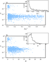 |
Fig. 8 Redshift prediction error and significance. (a) Scatter plot of the redshift relative error, δz, against the significance score, ∆χ2, for the test set. (b) Scatter plot of δz against the robustness score, R. |
4.3 Threshold on ∆χ2
Unlike MOS, where spectroscopy is carried out on preselected targets (e.g., photometrically selected), IFS provides spectroscopy of everything in the field of view. In MUSE surveys, sources must be blindly detected using algorithms such as ORIGIN (Mary et al. 2020) or FELINE (Wendt et al. 2025), which can produce many false positives in order to be highly complete. Currently, these false sources are processed by the redshift prediction pipeline just as in the case of real objects, and identified and marked as ZCONF0 during the visual inspection step (e.g., Bacon et al. 2023).
A reliable automatic redshift prediction tool must cope with these contaminants and classify them accordingly. Here, we investigate the ability of our method to discriminate between true and false sources, relying on the ∆χ2 significance score. Specifically, we applied our redshift prediction method to ZCONF0 spectra from the MXDF survey, and then compared their ∆χ2 predicted redshift significance score distribution with those of spectra having higher ZCONF scores taken from the same survey.
Figure 11 shows the distribution of log10 ∆χ2 for the 4 ZCONF classes. Looking at the four distributions, we can see that the significance score discriminates ZCONF2 and ZCONF3 classes from the ZCONF0 class, with almost no overlap. We note that ZCONF2 sources that overlap with ZCONF0 originate from spectra with a high fraction of negative values. ZCONF1 distribution, on the other hand, shows some overlap with ZCONF0 distribution. In this overlapping region, it becomes hard to distinguish between a very faint true source and a false one (e.g., originating from bad flat-fielding).
We observe that a threshold at log10 ∆χ2 = −2, allows us to keep all of the ZCONF2 and ZCONF3 sources and a large fraction of ZCONF1 sources, while rejecting most of the ZCONF0 sources. For this cut, we quote a completeness score4 of 95.9% and a purity score5 of 96.0%.
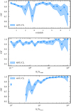 |
Fig. 9 Performance as a function of redshift and S/N for ZCONF 2 and 3 sources. (a) Average GF as a function of redshift, (b) GF as a function of the continuum S/N (S/Ncont), (c) GF as a function of the lines S/N (S/Nlines). The shaded regions indicate 68% Wilson confidence intervals. |
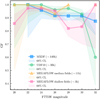 |
Fig. 10 Performance with varying depth. The different curves show the averaged GF in bins of the F775W magnitude for various surveys with different depths. Shaded regions indicate 68% Wilson confidence intervals. |
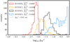 |
Fig. 11 Redshift significance score and ZCONF. log10 ∆χ2 distribution for the four classes of ZCONF in the MXDF survey. |
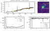 |
Fig. 12 Deblending MXDF-7381. Top-left: spectrum of MXDF-7381 ( fλ) in blue, best fit at z1 ( |


4.4 Application on blends
To ensure the robustness of our analysis, we deliberately excluded blended sources up to this point. For large-scale applications and studies involving deep fields, however, it becomes essential to identify and flag such blended sources, as they are ubiquitous (Melchior et al. 2021) and constitute a primary cause of incorrect redshift determinations. This is due to the fact that redshift pipelines (including ours) generally recover the redshift of the most luminous component (Baron & Poznanski 2016).
In this subsection, we explore the feasibility of blend detection based exclusively on 1D spectra using our learned-NMF basis vectors. We follow the framework described in Tsalmantza & Hogg (2012) with some adaptations. The method proceeds as follows:
- (a)
For a given spectrum, fλ, we predict its redshift using our method. We note the obtained χ2(z) curve,
 , and the corresponding redshift, z1. We note that if the spectrum is blended, this step identifies the redshift component exhibiting the strongest features.
 - (b)
We use pyPlatefit to fit the spectrum at z1, noting the fitted spectrum,
 . The goal of this step is, on the one hand, to maximally reduce reconstruction residuals; on the other hand, we also aim to fit rare lines not captured by our NMF basis vectors. If not accounted for, these rare lines would result in false blend detections. To this end, we extend the default line list used by pyPlatefit to include Fe II⋆, C II⋆ and Si II⋆ fluorescence emission lines, He I λ3187.745, He I λ4471.479, He I λ5875.624, and [N I] λ5200.257 emission lines.
 - (c)
Following the same steps in our redshift prediction method, we scan all possible redshifts a second time. This time, at each test redshift, we can augment our basis by injecting
 . We denote by
  the NMF basis vectors corresponding to redshift zi, where i indexes test redshifts. The augmented basis at zi is written as

At each zi, we nonnegatively project fλ into
 , and compute the reconstruction error, following the same equations in (5) and (6). We note the obtained χ2(z) curve
  .
. - (d)
We identify all minima in
 and discard minima that are in confusion with z1. If a minimum with ∆χ2 > tblend remains (as tblend is a threshold for class separation), we flag the spectrum as blended. The remaining minimum with the highest significance score ∆χ2 gives the blending redshift z2; we note the second reconstruction of the NMF
  .
.
These steps can be repeated to search for double or even triple blends. In this work, we stopped after one blend detection trial, as our goal has been to detect blends and not to estimate the number of mixing components. Figure 12 illustrates an example of a blended source detected by our approach.
We applied our deblending approach to all MXDF survey sources with a ZCONF of 1 or higher, for a total of 664 objects. We inspected all sources and flagged blended ones using the SourceInspector software and the AMUSED6 interface (Bacon et al. 2023)7. From the 664 objects, we flagged 183 as blended and removed 3 objects classified as stars.
For this test, we present the receiver operating characteristic curve (ROC curve) in Fig. 13. This curve reports the true positive rate (TPR) versus the false positive rate (FPR) for a series of thresholds (tblend) spanning 0.003–0.05 with a step of 0.001. TPR and FPR are defined as

where TP is the number of true positive detections (correctly predicted as blended), FP is the number of false positive detections (incorrectly predicted as blended), P is the total number of positive labels (number of blends), and N is the total number of negative labels (number of sources not blended). Next, we can quantify the performance based on the ROC curve and choose a threshold that best balances between the TPR and FPR.
To quantify the performance of our deblending approach, we used the area under the curve (AUC) score. Values close to 1 indicate excellent discrimination and, in our case, the AUC is 0.87, categorizing our method as displaying a “good” performance.
We selected the optimal threshold as the point that minimizes the Euclidean distance to the ideal classifier (0,1), resulting in a TPR of 0.78, a FPR of 0.18, and a threshold on ∆χ2 equal to 0.011. We note that this value is very close to the separation threshold between true and false sources (see Sect. 4.3).
Upon examining the classifications, we found that false positives mainly result from sky-subtraction residuals, bad pyPlatefit fits, and noise. Undetected blends at the optimal threshold correspond to very weak blends. Additionally, we observed that some blends remain undetected even at low thresholds (∆χ2 < 0.01). This occurs when a blending with one line coincides with a line of the first redshift, in which case pyPlatefit absorbs the blending line in step (b).
We conclude this subsection by suggesting possible improvements. Unlike Tsalmantza & Hogg (2012), who doubled the basis vectors at each test redshift (i.e., keeping one set fixed at the first redshift while the other slides with the test redshift), our approach augments the basis vectors using the pyPlatefit best fit at the first redshift. This strategy has the advantage of minimizing residuals at the location of spectral lines; however, it also results in the continuum being completely absorbed during the fit. Introducing a continuum model with fewer degrees of freedom could mitigate this issue and enable the detection of blended objects via continuum features. Additionally, exploiting the spatial origin of the emission would help identify cases in which a blending with one line coincides with another line of the first redshift.
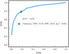 |
Fig. 13 Deblending test ROC curve. The TPR versus the FPR is plotted as a blue line. The value of the AUC score is shown, and the optimal threshold is marked by the green point. |
MUSE-WIDE DR2 survey test results.
4.5 Application to a new dataset
We tested our method on a new reduction of the MUSE-WIDE survey (DR2), which benefits from improved sky-subtraction and flat-fielding (Urrutia, in prep.). It also includes more sources: 2332 sources in DR2 compared to 1602 sources in DR1.
After inspecting all 2332 spectra and removing blends and spectra with very broad features, we obtained an overall GF of 97.1% on ZCONF2 and ZCONF3 classes. The GF of each ZCONF class is reported in Table 2. An inspection of the failed predictions reveals that the majority of them are due to confusion between [O II] and Lyα.
4.6 Implementation and computational time
We have made the data matrix used in this work available, along with the implementation of the nearly NMF algorithm and the code for our redshift prediction method in a Julia package Moose.jl, along with a Python wrapper. Our implementation takes approximately 200 ms to test 7000 redshifts for a single input spectrum; the code was run on a 24-threads CPU with multithreading applied to parallelize multiple redshift tests. This time can be reduced in a number of ways: by decreasing the resolution δΓ of the basis vectors, by selecting redshifts to test if prior information is available, or by the use of a CPU with more threads. Such a computation time is reasonable for current MUSE surveys.
5 Discussion
In this study, we demonstrate that learning a rest-frame representation of galaxy spectra through NMF in a data-driven setup provides an effective framework for automated redshift estimation. By projecting new spectra onto this representation under nonnegativity constraints and identifying the best-fitting decomposition, our method attained an overall success rate of 93.7% when applied to MUSE spectra. To further quantify the reliability of each measurement, we introduced a ∆χ2 score; adopting a threshold at ∆χ2 = 0.01 yielded a very good separation between ZCONF0 and higher-confidence redshifts, illustrating the robustness of our approach against false detections (ZCONF0), which are common in IFS data. Finally, we assessed the feasibility of blend detection using our NMF basis and showed that approximately 78% of blended objects can be recovered at a false positive rate of 18%.
Because standard redshift inference tools have been developed and tested primarily on low-redshift spectra (z<3), we did not attempt a direct numerical comparison. Rather, we emphasize that our method has been applied here to MUSE spectra spanning redshifts between 0 and 6.7, a range that presents significant challenges: line confusion such as Lyα with [O II] and Lyα with Hα, as well as the redshift desert. Achieving an overall 93.7% success rate across this regime demonstrates that our method is robust under conditions that are not systematically addressed by existing tools.
Next, we compare our method with the methodological choices in established approaches. Classical tools, such as RedRock, estimate redshifts by fitting a set of archetype templates constructed from a combination of observed and synthetic spectra, whereas our method learns the templates directly from the data, enabling it to adapt to the diversity of the sample. AUTOZ, on the other hand, relies on cross-correlation with a set of SDSS templates, which requires subtracting the stellar continuum and discards physically informative broadband features. Cross-correlation also suffers from well-known issues, including template mismatch, ambiguous peaks in the cross-correlation function when a spectrum is dominated by a single emission line, and reduced robustness when spectra deviate from the assumed template family. In comparison, our method leverages the full stellar continuum, which constitutes a discriminative source of information, especially when separating between Lyα and [O II]. Recent deep-learning approaches, such as GaSNet III and M-TOPnet, train neural networks to predict redshifts using strategies such as multitask learning and representation learning. While these networks achieve high performance, they require large labeled datasets (>20 000 spectra) for training, and typically operate on continuum-subtracted inputs, which again removes potentially discriminative information. In contrast, our method requires far fewer training examples (≲7000) and processes the full spectrum, making it both competitive with and complementary to these approaches.
Despite its robustness, our method has limitations. We find reduced performance in spectra affected by artifacts such as: (1) residuals from imperfect sky subtraction; (2) flat-fielding errors that distort the continuum; and (3) spectra with a negative median flux, where NNLS decompositions often fail. Because such artifacts are unavoidable in IFS data, a promising direction is to replace the NNLS solver with a neural network (e.g., encoder-like architecture) that enforces nonnegativity, while learning to ignore such artifacts, potentially leading to further performance gains.
6 Conclusions
In this work, we presented a method for automatic redshift prediction for MUSE galaxy spectra. These spectra span a wide redshift range (0 < z < 6.7), where classic tools perform poorly or have not been systematically tested. The method learns a low-rank representation through nonnegative matrix factorization and estimates redshifts by projecting new spectra onto this basis and evaluating χ2 errors across trial redshifts.
Using a K-fold cross-validation, we identified ten basis vectors as the optimal representation, and our method achieved a good fraction of 93.7% on an independent test set. Most of the failed predictions resulted from confusion between the [O II] doublet and Lyα. To assess the reliability of a prediction, we introduced two metrics: the significance score, ∆χ2, and the robustness score, R. We found that failed predictions are typically associated with low values of both metrics, with R showing good discriminating power.
We demonstrated an application of our method to spectral deblending. The approach first identifies and fits the dominant redshift component, then re-scans for secondary redshift solutions after augmenting the NMF basis with the fitted spectrum. When applied to MXDF sources, the method achieves a strong level of performance, recovering 78% of blended sources with a false positive rate of 18%.
Applied to a dataset with improved reduction, the method reached a good fraction of 97.1% on sources with ZCONF2 and ZCONF3, demonstrating robust generalization and sensitivity to data quality. We further evaluated its ability to identify false detections and showed that a threshold at ∆χ2 = 0.01 efficiently separates genuine from spurious sources.
Overall, these results demonstrate that low-rank representations obtained via NMF provide a flexible and data-driven framework for automated redshift determination across a broad redshift range. In addition to high accuracy, the method offers intrinsic reliability diagnostics, making it well-suited to applications in current and coming large spectroscopic surveys.
Acknowledgements
We thank A. Casey for fruitful discussions in the initial phases of the project. NB acknowledges support from the ANR DARK grant (ANR-22-CE31-0006). MB acknowledges support from the Blaise Pascal GPU computing infrastructure. TU acknowledges funding from the European Research Council (ERC) under the European Union’s Horizon 2020 research and innovation programme (grant agreement 101020943, SPECMAP-CGM). Part of this work was supported by the German Deutsche Forschungsgemeinschaft, DFG project number Ts 17/2-1.
References
- Anand, A., Guy, J., Bailey, S., et al. 2024, AJ, 168, 124 [NASA ADS] [CrossRef] [Google Scholar]
- Bacon, R., Accardo, M., Adjali, L., et al. 2010, SPIE Conf. Ser., 7735, 773508 [Google Scholar]
- Bacon, R., Conseil, S., Mary, D., et al. 2017, A&A, 608, A1 [NASA ADS] [CrossRef] [EDP Sciences] [Google Scholar]
- Bacon, R., Brinchmann, J., Conseil, S., et al. 2023, A&A, 670, A4 [NASA ADS] [CrossRef] [EDP Sciences] [Google Scholar]
- Baldry, I. K., Alpaslan, M., Bauer, A. E., et al. 2014, MNRAS, 441, 2440 [Google Scholar]
- Baron, D., & Poznanski, D. 2016, MNRAS, 465, 4530 [Google Scholar]
- Blanton, M. R., & Roweis, S. 2007, AJ, 133, 734 [NASA ADS] [CrossRef] [Google Scholar]
- Bolton, A. S., Schlegel, D. J., Aubourg, É., et al. 2012, AJ, 144, 144 [NASA ADS] [CrossRef] [Google Scholar]
- Bouché, N. F., Wendt, M., Zabl, J., et al. 2025, A&A, 694, A67 [NASA ADS] [CrossRef] [EDP Sciences] [Google Scholar]
- Bro, R., & De Jong, S. 1997, J. Chemom, 11, 393 [Google Scholar]
- Cirasuolo, M., Fairley, A., Rees, P., et al. 2020, Messanger, 10 [Google Scholar]
- Dalton, G., Trager, S., Abrams, D., et al. 2012, in Proc. SPIE, 8446 [Google Scholar]
- DESI Collaboration (Abareshi, B., et al.) 2022, AJ, 164, 207 [NASA ADS] [CrossRef] [Google Scholar]
- de Jong, R. S., Agertz, O., Berbel, A. A., et al. 2019, Messenger, 175, 3 [Google Scholar]
- Epinat, B., Contini, T., Mercier, W., et al. 2024, A&A, 683, A205 [NASA ADS] [CrossRef] [EDP Sciences] [Google Scholar]
- Ginolfi, M., Mannucci, F., Belfiore, F., et al. 2025, A&A, 693, A73 [NASA ADS] [CrossRef] [EDP Sciences] [Google Scholar]
- Green, D., & Bailey, S. 2024, ITSP, 72, 5187 [Google Scholar]
- Hinton, S., Davis, T. M., Lidman, C., Glazebrook, K., & Lewis, G. 2016, A&C, 15, 61 [Google Scholar]
- Hurley, P. D., Oliver, S., Farrah, D., Lebouteiller, V., & Spoon, H. W. W. 2013, MNRAS, 437, 241 [Google Scholar]
- Inami, H., Bacon, R., Brinchmann, J., et al. 2017, A&A, 608, A2 [NASA ADS] [CrossRef] [EDP Sciences] [Google Scholar]
- Kohavi, R. 1995, in Proc. 14th Int. Joint Conf. Artificial Intelligence, 1137 [Google Scholar]
- Lee, D. D., & Seung, H. S. 1999, Nature, 401, 788 [Google Scholar]
- Mary, D., Bacon, R., Conseil, S., Piqueras, L., & Schutz, A. 2020, A&A, 635, A194 [EDP Sciences] [Google Scholar]
- Melchior, P., Joseph, R., Sanchez, J., MacCrann, N., & Gruen, D. 2021, NatRP, 3, 712 [Google Scholar]
- Tsalmantza, P., & Hogg, D. W. 2012, ApJ, 753, 122 [Google Scholar]
- Urrutia, T., Wisotzki, L., Kerutt, J., et al. 2019, A&A, 624, A141 [NASA ADS] [CrossRef] [EDP Sciences] [Google Scholar]
- Wendt, M., Henschel, M., & Soth, O. F. 2025, JOSS, 10, 7528 [Google Scholar]
- York, D. G., Adelman, J., Anderson, J. E., Jr., et al. 2000, AJ, 120, 1579 [NASA ADS] [CrossRef] [Google Scholar]
- Zhong, F., Napolitano, N. R., Heneka, C., et al. 2025, MNRAS, 543, 691 [Google Scholar]
- Zhu, G. 2016, arXiv e-prints [arXiv:1612.06037] [Google Scholar]
As discussed in Bacon et al. (2023), redshifts were obtained using a semi-automatic procedure where the five best redshift solutions produced by a MUSE-adapted version of the MARZ algorithm were visually inspected by a group of experts, who evaluated the reliability of the redshift on a scale from 0 to 3: a ZCONF of 3 indicates a secure redshift from multiple spectral lines; 2 represents a highly probable redshift from a single high S/N line or from multiple low-S/N lines; 1 denotes a possible redshift from a low S/N line; and 0 is attributed when the redshift is undetermined.
Matrix Y changes during iterations and can be different for W and H updates but does not need to be computed explicitly. As explained in Green & Bailey (2024), Y appears implicitly in Eq. (3) via the [ ]+ and [ ]− operators.
Note: our definitions for the redshift significance and robustness scores differ from other definitions in SDSS or DESI literature.
Fraction of ZCONF 1, 2 or 3 sources that are successfully selected.
Fraction of selected sources that are truly ZCONF 1, 2, or 3.
SourceInspector enables interactive inspection of narrow-band images and localization of emission within the datacube, while AMUSED provides an efficient way to identify nearby sources.
All Tables
All Figures
|
Fig. 1 Main statistical properties of the selected MUSE galaxy sample. Distributions of (a) redshift; (b) redshift confidence score (ZCONF)’ (c) stellar continuum S/N (S/Ncont), and (d) emission and absorption lines collective S/N (S/Nlines). |
| In the text | |
|
Fig. 2 MUSE galaxy spectra matrix in the rest frame. This matrix shows selected MUSE galaxy spectra, prepared for NMF decomposition. Spectra are sorted by increasing redshift (from bottom to top) and transformed to their rest frame. Key redshifts are shown on the y-axis and important spectral lines are indicated on top of the figure. The color of each pixel encodes flux density, scaled using a 95% z-scale to enhance the visibility of emission lines. Bluer colors represent higher flux densities; white pixels denote missing or unobserved data. |
| In the text | |
|
Fig. 3 Illustration of redshift prediction with NMF basis vectors. (a) Rest-frame spectrum of the UDF10-4 source at redshift 0.7649 in blue. This galaxy exhibits stellar continuum, strong [O II], Hβ, and [O III] spectral emission lines (their locations are indicated on top of the figure); the best NMF reconstruction is plotted in black. (b) Corresponding χ2 curve, the minimum happens at the true redshift (vertical red dashed line), hence, successfully predicting the correct redshift. The second minimum in the χ2 curve at z ∼ 4.4 corresponds to a solution in which [O II] gets mistaken to be Lya. The values of the ∆χ2 and R metrics are also reported in (b); their values indicate a significant minimum and a very robust redshift prediction. |
| In the text | |
|
Fig. 4 NMF rank selection. Top and bottom panels: Mean GF and mean MAE with outlier rejections across the test folds, respectively, for ranks of 6–13. Corresponding standard deviations are shown as error bars. Both metrics are reported for spectra with ZCONF values of 2 and 3. |
| In the text | |
|
Fig. 5 NMF-learned basis vectors. Panel a shows the basis vectors obtained from a sequential rank–10 NMF decomposition applied to 80% of the sample. The index n labels each basis vector. The names and rest-frame wavelengths of prominent spectral emission and absorption lines are indicated in the upper panels. Panel b presents zoomed-in views of the [O II] and Lyα emission lines, shown in the first and second columns, respectively. In each zoom-in, the line’s peak flux is normalized to one, the line rest wavelength is shown with a vertical dashed gray line, and the corresponding basis vector is indicated. |
| In the text | |
|
Fig. 6 Redshift prediction workflow using a rest-frame representation learned with nearly NMF. |
| In the text | |
|
Fig. 7 Scatter plot of the predicted redshift (zp) against true redshift (zt) for the test set. Dashed gray lines mark predicted redshifts for [O II] sources misidentified as Lyα sources and vice versa. |
| In the text | |
|
Fig. 8 Redshift prediction error and significance. (a) Scatter plot of the redshift relative error, δz, against the significance score, ∆χ2, for the test set. (b) Scatter plot of δz against the robustness score, R. |
| In the text | |
|
Fig. 9 Performance as a function of redshift and S/N for ZCONF 2 and 3 sources. (a) Average GF as a function of redshift, (b) GF as a function of the continuum S/N (S/Ncont), (c) GF as a function of the lines S/N (S/Nlines). The shaded regions indicate 68% Wilson confidence intervals. |
| In the text | |
|
Fig. 10 Performance with varying depth. The different curves show the averaged GF in bins of the F775W magnitude for various surveys with different depths. Shaded regions indicate 68% Wilson confidence intervals. |
| In the text | |
|
Fig. 11 Redshift significance score and ZCONF. log10 ∆χ2 distribution for the four classes of ZCONF in the MXDF survey. |
| In the text | |
|
Fig. 12 Deblending MXDF-7381. Top-left: spectrum of MXDF-7381 ( fλ) in blue, best fit at z1 ( |
| In the text | |
|
Fig. 13 Deblending test ROC curve. The TPR versus the FPR is plotted as a blue line. The value of the AUC score is shown, and the optimal threshold is marked by the green point. |
| In the text | |
Current usage metrics show cumulative count of Article Views (full-text article views including HTML views, PDF and ePub downloads, according to the available data) and Abstracts Views on Vision4Press platform.
Data correspond to usage on the plateform after 2015. The current usage metrics is available 48-96 hours after online publication and is updated daily on week days.
Initial download of the metrics may take a while.