| Issue |
A&A
Volume 709, May 2026
|
|
|---|---|---|
| Article Number | A193 | |
| Number of page(s) | 14 | |
| Section | Extragalactic astronomy | |
| DOI | https://doi.org/10.1051/0004-6361/202558635 | |
| Published online | 13 May 2026 | |
Predicting CO and dust emission of star-forming galaxies
Extension to star-forming low-mass and dwarf galaxies
1
Université de Strasbourg, CNRS, Observatoire Astronomique de Strasbourg, UMR 7550, 67000 Strasbourg, France
2
Laboratoire d’Astrophysique de Bordeaux, Univ. Bordeaux, CNRS, B18N, allé Geoffroy Saint-Hilaire, 33615 Pessac, France
3
Astronomical Observatory, Jagiellonian University, ul. Orla 171, 30-244 Kraków, Poland
★ Corresponding author: This email address is being protected from spambots. You need JavaScript enabled to view it.
Received:
18
December
2025
Accepted:
31
March
2026
Abstract
In this work, we investigate whether dwarf galaxies differ from spirals and whether star formation produces radio and far-infrared (FIR) emission in the same way as it does for spiral galaxies. Radio, FIR, and CO emission depend on gas density, temperature, magnetic field strength, and metallicity. The radio-FIR correlation and Schmidt-Kennicutt relation characterize the links for Milky Way-like galaxies. However, in this work, we want to investigate whether they also hold for smaller objects with different morphologies. Here, we extend our previous work on the IR, line, and radio emission of local and high-z galaxies to local star-forming low-mass and dwarf galaxies. The calculation of the cosmic ray (CR) densities were improved compared to the previous version of the model. The CR ionization rate we found for the different galaxy samples is higher by a factor of 3 than the rate determined for the solar neighborhood. This means that the mean yield of low-energy CR particles is three times higher in external galaxies than what was observed by Voyager I. The dependence of the N(H2)/ICO factor on the metallicity and stellar mass are calculated by the model. The weaker CO emission from low-metallicity galaxies is due to the large amount of (CO-dark) H2 surrounding the regions where CO is not photodissociated. Within our model framework, star-forming low-mass and dwarf galaxies follow the radio-IR correlation.
Key words: galaxies: dwarf / galaxies: general / galaxies: ISM / galaxies: star formation
© The Authors 2026
 Open Access article, published by EDP Sciences, under the terms of the Creative Commons Attribution License (https://creativecommons.org/licenses/by/4.0), which permits unrestricted use, distribution, and reproduction in any medium, provided the original work is properly cited.
This article is published in open access under the Subscribe to Open model. This email address is being protected from spambots. You need JavaScript enabled to view it. to support open access publication.
1. Introduction
The radio-infrared (radio-IR) correlation and the Schmidt-Kennicutt relation between the molecular gas mass and the star formation rate (SFR) are well established in star-forming (SF) galaxies with stellar masses higher than ∼109 M⊙ (see, e.g., Yun et al. 2001; Bell 2003; Molnár et al. 2021; Kennicutt & De Los Reyes 2021; Schinnerer & Leroy 2024). The question of whether these relations also hold in SF low-mass and dwarf galaxies is still matter of debate. The physical conditions in these low-mass and low-metallicity galaxies are distinct from those of their high-mass counterparts. Observationally, the quality of using the radio continuum, IR emission, and CO emission as tracers of the different ISM components depends on many factors, such as gas density, temperature, magnetic field strength, and metallicity.
Detecting CO in dwarf galaxies has been notoriously difficult (e.g., Leroy et al. 2009; Cormier et al. 2014) because of the faintness of the CO emission. Low metallicity environments imply lower C and O abundances and low dust-to-gas ratios (Draine et al. 2007). This decreases the H2 abundance since H2 molecules form on dust surfaces. Dust provides much of the far-UV shielding that is necessary to prevent CO, which generally provides little self-shielding, from photodissociating (Bolatto et al. 2013). Model predictions point to a CO deficiency in low-metallicity SF galaxies as being due to a decrease in dust-shielding, which leads to strong photodissociation of CO by the intense UV radiation fields that are generated in the SF regions (e.g., Wolfire et al. 2010). On the other hand, H2 photodissociates via the absorption of FUV photons and, for moderate AV, this can lead to them becoming optically thick, allowing H2 to become self-shielded from photodissociation (e.g., Gnedin & Draine 2014), leaving a potentially significant reservoir of H2 existing outside of the CO-emitting core, which is commonly called CO-dark molecular gas. As a consequence, the CO-H2 conversion factor strongly increases with decreasing metallicity (e.g., Ramambason et al. 2024). Within the CO-dark photodissociation regions [C II]158 μm emission can be used as a tracer of molecular hydrogen (e.g., Madden et al. 2020).
Many authors have reported that the SF law derived for spiral galaxies does not hold in dwarf galaxies, suggesting the existence of different regimes of SF for different galaxy types. The SF surface densities of dwarf galaxies tend to be lower than the values expected from the Schmidt-Kennicutt relation (Wyder et al. 2009; Gatto et al. 2013; Roychowdhury et al. 2015, 2017; de los Reyes & Kennicutt 2019 but see Teich et al. 2016 for a different conclusion). These studies are based on the atomic gas surface density.
Using CO emission to trace H2 is difficult in low-metallicity (generally low-mass) galaxies because the CO emission per H2 mass is much lower, meaning that the CO-H2 conversion factor, αCO, is higher than in large spirals. Different methods to estimate αCO in dwarf galaxies have yielded discordant values (e.g., Leroy et al. 2011; Bolatto et al. 2013; Hunt et al. 2015; Amorín et al. 2016; Madden & Cormier 2019); hence, it is difficult to estimate the H2 content of low-metallicity galaxies. Cloud-resolved studies of the small local group galaxies M 33 and NGC 6822 suggest that molecular gas is converted in stars more quickly; namely, involving a lower H2 depletion time (Gardan et al. 2007; Gratier et al. 2010, 2017) than in large spirals. This is to be expected because of the weaker stellar winds (Dib 2011) and higher density for conversion of H I to H2 at low metallicities.
The radio continuum emission is emitted by ionized gas, as well as through cosmic rays (CR) interacting with magnetic fields (synchrotron emission). The radio continuum emission at centimeter wavelengths is generally produced by a combination of free–free emission from thermal electrons and nonthermal synchrotron emission from relativistic electrons spiraling around magnetic fields (e.g., Condon 1992). Increased ionizing UV photon production, low metallicity, and reduced dust absorption can increase the ionization of the gas (and, hence, the thermal emission component). This effect is counteracted by increased ionizing photon escape from the galaxy (e.g., Fernandez & Shull 2011; Benson et al. 2013; Leitherer et al. 2016). Together with the SFR, the gravitational potential determines the CR loss versus injection budget: the SF surface density threshold to drive winds and outflows, which can be responsible for CR advection and escape from the galaxy, is lower in smaller gravitational potential wells. Thus, it is not obvious that the radio-IR correlation holds for SF low-mass and dwarf galaxies.
In this paper, we apply the model of IR, molecular line, and radio continuum emission presented in Vollmer et al. (2017, 2022, and 2025) to the sample of SF low-mass and dwarf galaxies presented in Leroy et al. (2008 and 2009). We investigated if the model can reproduce the available integrated IR, CO, and radio continuum observations. Since the CO-H2 conversion factor is calculated by the model, the mechanism for its increase with decreasing metallicity can be identified within the model framework.
The article is structured in the following way: the new galaxy sample and the model are introduced in Sect. 2 and Sect. 3. The model results are presented and compared to available observation in Sect. 4. The implications on the CO conversion factor, the CO-dark gas, the thermal fraction of the radio continuum emission, the SF law, and the viscous gas transport are discussed in Sect. 5, followed by our conclusions in Sect. 6.
2. The star-forming low-mass and dwarf galaxy sample
We applied our models to the the galaxy sample presented in Leroy et al. (2008). In their study, these authors used H I maps from the H I Nearby Galaxy Survey (THINGS) and CO maps measured by the HERA CO-Line Extragalactic Survey and the Berkeley-Illinois-Maryland Association Survey of Nearby Galaxies. Their galaxy sample was divided in two parts: high- and low-mass galaxies. Models of galaxies with stellar masses higher than 1010 M⊙ were presented in Vollmer et al. (2017, 2022, and 2025). The galaxies of masses 107 ≤ M* ≤ 1010 M⊙ are presented here (Table 1). The rotation velocities range between 50 and 130 km s−1. The metallicities vary between 12+log(O/H) = 7.5–8.5 (Fig. A.1). The CO data were provided by the HERACLES survey (Leroy et al. 2009).
Galaxy sample.
In addition, we applied our model to the galaxy samples described in Vollmer et al. (2017, 2025): local luminous IR galaxies (LIRGs; Fisher et al. 2019), local starbursts (i.e., ULIRGs; Downes & Solomon 1998), intermediate-redshift (z ∼ 0.3 − 0.5) main sequence (MS) galaxies (PHIBSS2; Freundlich et al. 2019), high-z MS galaxies (PHIBSS, Tacconi et al. 2013), and starburst galaxies (Genzel et al. 2010).
3. The model
Galactic gas disks are modeled as turbulent clumpy SF accretion disks. The details of the gas disk model are described in Appendix D. The turbulent nature of the ISM is taken into account by applying scaling relations for the gas density and velocity dispersion to gas clouds of given sizes. The scaling relations change when the clouds become self-gravitating. The cloud temperature is calculated via the balance of heating and cooling. In this way, the gas density, temperature, and velocity dispersion were determined for each cloud. The molecular abundances depend on the density, temperature, and CR ionization rate. The CR ionization rate was calculated by using a steady-state model (Pohl 1993) calibrated by the CR ionization in the solar neighborhood. The molecular abundances were derived from calculations by the time-dependent gas-grain code Nautilus (Hersant et al. 2009; Ruaud et al. 2016). The molecular abundances, gas density, velocity dispersion, and temperature served as input for the calculation of the molecular line emission. The radio continuum emission was calculated via a steady-state model calibrated by the observed IR-radio correlations. We performed simulations to predict the emission at many different wavelengths of observed galaxies.
The model simultaneously calculates radial profiles of the gas surface density Σ, the SF surface density  , the gas velocity dispersion, and the volume-filling factor, all of which are large-scale properties; at small scales, it calculates fmol and the IR spectral energy distribution (SED) as well as the molecular line emission via RADEX (van der Tak et al. 2007). For the details of our analytical model, we refer to Appendix A of Lizée et al. (2022). The stellar mass profile is given by the Sérsic fit to the observations, so the calculations are of the gas distribution and kinematics.
The rotation curve and the surface density profile of the stellar disk served as model inputs. For the low-mass and dwarf galaxies we added a dark matter halo with a cored isothermal density profile,
 (1)
(1)
where we adapted ρ0 and R0 to obtain, together with the stellar disk, the observed rotation curve given by Leroy et al. (2008). The central densities and core radii are given in Table 1 for the different galaxies. The halo is also taken into account for the vertical hydrostatic equilibrium.
The model contains three main free parameters: (i) the Toomre parameter  of the gas, where a Q < 1 disk is gravitationally unstable; (ii) the external accretion rate Ṁ, where an increasing Ṁ at constant Q increases vturb; and (iii) δ = ldriv/lcl, where lcl is the cloud size scale and ldriv is the driving length of the turbulence. The mass accretion rate and δ are assumed to be constant. Given the Toomre parameter, mass accretion rate, rotation curve, and stellar mass surface density and velocity dispersion, the large-scale accretion disk model yields the gas density, disk height, gas surface density, gas turbulent velocity dispersion, and SF surface density. The turbulent nature of the interstellar medium (ISM) is taken into account by applying scaling relations for the gas density and velocity dispersion to gas clouds of given sizes. The scaling relations change when the clouds become self-gravitating. The cloud temperature is calculated via the balance of heating and cooling. In this way, the gas density, temperature, and velocity dispersion were determined for each cloud. The molecular abundances depend on the density, temperature, and CR ionization rate. The molecular abundances, gas density, velocity dispersion, and temperature served as input for the calculation of the molecular line emission. The radio continuum emission was calculated via the steady-state model of Pohl (1993) calibrated by the observed IR-radio correlations. For each radius R, the model yields the SF surface density
  , the H I emission, and the IR continuum and molecular line emission for a given set of Q, Ṁ, and δ. Lizée et al. (2022) showed that these radial profiles do not significantly depend on δ for 2 ≤ δ ≤ 10. We thus set δ = 5. The constant that links the rate of energy injection by supernovae to the SFR was set at ξ = 9.2 × 10⁻⁸ (pc yr−1)2. The details of the gas disk model are described in Appendix A of Vollmer et al. (2025).
Following Vollmer et al. (2017), our leaky-box model used an effective yield, meaning that enriched gas can escape and be accreted from the circumgalactic medium. This leads to a gas metallicity of
 (2)
(2)
with
 (3)
(3)
where Σ* is the stellar mass surface density. The normalization of Eq. (2) is half that of the high-mass galaxies (Vollmer et al. 2017, 2022, 2025), which reproduced the integrated metallicities given by McQuade et al. (1995), Kennicutt et al. (2011), and Madden et al. (2013). The observed metallicities of all galaxies more massive than Ho I were reproduced within 1σ ≲ 0.1 dex (Fig. A.1). Those of DDO 154 and Ho I were underestimated by 0.3 dex and 0.5 dex, respectively.
To determine the chemical abundances, we used seven grids calculated by the time-dependent gas-grain code Nautilus (Hersant et al. 2009; Ruaud et al. 2016) for CR ionization rates of (0.1, 0.3, 1.3, 3.0, 6.5, 30, 130, 650, 6500)×10−17 s−1. We varied the time, gas density, and gas temperature. The chemical abundances were calculated by interpolating the 4D Nautilus grid for a given CR ionization rate (Sect. 3.1) and solar metallicity.
The abundances scale with the model metallicity. Since Nautilus is designed to calculate the molecular abundances in gas with n ≳ 103 cm−3, the Nautilus abundances were extrapolated to lower densities. This extrapolation only affects the CO emission of the local non-starburst galaxies, particularly the low-mass and dwarf galaxies. We validated our approach by recalculating the CO(1-0) emission of these galaxies using the simple phenomenological model of CO formation as the immediate descendant of quiescently recombining HCO+ (Eq. (4c) of Liszt 20071). Changes in the model CO(1-0) fluxes are less than ∼10% for all galaxies, except for the case of DDO 154, where the recalculated flux is ∼40% lower than the initial flux. These changes are well within the uncertainties of the model. In addition, the photodissociation of H2 and CO molecules (CO-dark gas) in the outer envelopes of gas clouds, following the approach of Krumholz et al. (2008, 2009) and Wolfire et al. (2010), was included in our model (see Appendix E).
The line emission was calculated with RADEX using the inputs as calculated above. The total emission is highly dependent on the gas mass surface densities (and, hence the filling factors). These come from the local gas densities and the prescription that determines whether gas is atomic or molecular based on the competition between the molecular formation time and the freefall time. The details are described in Sects. 2.1.1 and 2.4 of Vollmer et al. (2017).
3.1. Cosmic-ray ionization rate
Cosmic rays with energies above 1 MeV interact with atoms and molecules of the interstellar medium. These high-energy particles can directly ionize a species. This direct process is dominant for H2, H, O, N, He, and CO. Electrons produced in the direct process can cause secondary ionization before they are thermalized. In addition to secondary ionization, the electrons produced in direct CR ionization can electronically excite molecular and atomic hydrogen. The radiative relaxation of H2 (and H) produces UV photons that ionize and dissociate molecules. While direct ionization is dominant for CO, secondary ionization and dissociation are dominant for HCN. The CR ionization rate thus affects the chemical abundances.
As in Vollmer et al. (2025), we calculated the CR ionization rate and then injected it into Nautilus, which uses the total H2 CR ionization rate ζH2 as input (Wakelam et al. 2012). The CR nucleons (mainly protons) lose energy by the combined effects of ionization and Coulomb losses, adiabatic deceleration, and pion production. To calculate the local (solar neighborhood) CR density spectra of electrons and protons, we followed Pohl (1993). The normalization factors of the proton spectrum was chosen such that the observed local CR intensity, averaged over a solid angle, J(E), was recovered (Fig. 3 of Vollmer et al. 2025). To calculate the CR ionization rate at a given distance R from the center of a galaxy, we set nH to the gas density of the analytical galaxy model (Appendix D), use the interstellar radiation field U and the magnetic field strength of the galaxy model at R, and multiply the proton and electron spectra by  of the galaxy model. In the Vollmer et al. (2025) the normalization was done with the SF surface density,
  .
.
We took a closer look at the CR ionization rates at the scale lengths of the stellar disks. On average, the new normalisation led to CR ionisation rates about five times higher in local MS, LIRGs, and starburst galaxies. The increase in the CR ionization rates was about a factor of 2–3 in the intermediate-redshift LIRGs and high-redshift MS galaxies, whereas it was negligible in the high-z starburst galaxies. However, this only led to a maximum increase in CO(1-0) line emission by ≲50% across all sample galaxies. We note that the increase in the CO line emission is greater for higher transitions. The CO(4-3) line emission increased by about a factor of 1.5–2. On the one hand, an increased CR ionization rate leads to a lower CO abundance. On the other hand, it increases the CR gas heating. As CO emission increased with increasing CR ionization rate, the effect of the gas heating dominates.
3.2. Radio continuum
Overall, CR electrons are accelerated to relativistic velocities in expanding supernova (SN) shells. The exponent of the CRe injection spectrum is q = 2.3, as expected for superbubbles created by multiple SN remnants (Vieu et al. 2022). For relativistic electrons, ionization and Coulomb losses, nonthermal bremsstrahlung, adiabatic deceleration, inverse Compton losses, and synchrotron emission have to be taken into account (e.g., Lacki et al. 2010). The normalization factor of the electron spectrum was chosen such that the observed local CR intensity, averaged over a solid angle was recovered (Fig. 3 of Vollmer et al. 2025). To calculate the CR ionization rate at a given distance R from the center of a galaxy, we set the gas density, nH, to the gas density of the analytical galaxy model, using the interstellar radiation field U and the magnetic field strength of the galaxy model at R, and normalized the equilibrium spectrum of CR protons and electrons with the SF volume density,  , of the galaxy model.
Following Vollmer et al. (2022), we assumed a stationary CR electron density distribution (∂n/∂t = 0). The CR electrons are transported into the halo through diffusion or advection where they lose their energy via adiabatic losses or where the energy loss through synchrotron emission is so small that the emitted radio continuum emission cannot be detected. Furthermore, we assumed that the source term of CR electrons is proportional to the SFR volume density,  . For the energy distribution of the CR electrons, the standard assumption is a power law with index, q, which leads to a power law of the radio continuum spectrum with index −(q − 1)/2 (e.g., Beck 2015). The details of the radio continuum model are described in Appendix B of Vollmer et al. (2025).
As a supplementary step, we replaced Eq. (B.11) of Vollmer et al. (2025) by calculating the radio continuum emission according to chapter 5 of Condon & Ransom (2016) and chapter 3 of Pacholczyk (1970). For the CR energy loss terms we used the formalism of Pohl (1993) with the energy loss time scales of Vollmer et al. (2022). The new method has the advantage that the normalization of the CR ionization rate and yield of low-energy CR particles are explicitly set within the model framework; they are three times higher than what was observed by Voyager I and very close to the results presented in Vollmer et al. (2025).
4. Model result
The model calculates the IR SED, CO emission, and the radio-continuum SEDs. These are compared to available observations in Sects. 4.1, 4.2, and 4.3, respectively.
4.1. Infrared emission
Following Vollmer et al. (2017), we extracted all available photometric data points for our galaxy samples from the CDS VizieR database2 for a direct comparison between the model and the observed dust SED. Since the flux densities were determined within different apertures, we only took the highest flux densities for a given wavelength range around a central wavelength of λ0 (0.75 ≤ λ/λ0 ≤ 1.25). In this way, only the outer envelope of the flux density distribution was selected. We also separately show the Herschel measurements from Dale et al. (2012). Since our dust model does not include stochastically heated small grains and PAHs, the observed IR flux densities for λ ≲ 50 μm cannot be reproduced by the model. We assumed a dust mass absorption coefficient, taking the form of
 (4)
(4)
with λ0 = 250 μm, κ0 = 0.48 m2 kg−1 (Dale et al. 2012) and a gas-to-dust ratio of  (including helium; Rémy-Ruyer et al. 2014). The exponent was β = 1.5 for the SF low-mass and dwarf galaxies. The corresponding model and observed 10–1000 μm luminosities (hereafter, TIR) and dust IR SEDs are presented in Figs. 1 and B.1. The observed TIR luminosities are taken from Kennicutt et al. (2011), Dale et al. (2012), Rujopakarn et al. (2013), Cormier et al. (2015), Rémy-Ruyer et al. (2015), and Aniano et al. (2020). Overall, the model and observed TIR luminosities agree within a factor of 2. Most of the model TIR luminosities of the local MS galaxies (small and large crosses in Fig. 1) are underestimated by about 50%.
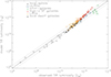 |
Fig. 1. Model TIR luminosity as a function of the observed TIR luminosity. The dotted lines show a factor two above and below the equality. |
As for the TIR luminosities, the observed IR SEDs are reproduced by the model within a factor of 2. The model IR SEDs of Ho I and Ho II are somewhat overestimated, whereas that of NGC 925 is somewhat underestimated. Since the uncertainty of our model results is about a factor of 2 (Vollmer et al. 2017), we did not try to adjust the SFR of the sample galaxies to obtain model results closer to observations. We fit modified Planck functions with β = 1.5 to the model dust IR SEDs to derive the dust temperatures. The modified Planck functions are shown as dashed red lines in Fig. B.1. The resulting mean temperatures of the large grain population lie within 13 and 23 K with a mean of 19 ± 3 K.
4.2. CO emission
Since the CO emission of SF low-mass and dwarf galaxies is notoriously low, as stated in Sect. 1, the CO emission has only been detected in five out of 11 galaxies (Leroy et al. 2009, 2022). Upper limits are available for four galaxies. The model and observed CO(2-1) luminosities and upper limits are shown in Fig. 2. The model overpredicts the observed CO luminosities by about 50%. The model CO luminosities are consistent with the observed upper limits, while Ho II probably is close to the detection limit. We also calculated models with half the gas metallicities. These models resulted in about 50% lower CO luminosities and reproduce the observed CO luminosities within a factor of 2, which is within the model uncertainties (Vollmer et al. 2017).
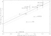 |
Fig. 2. Model CO luminosity as a function of the observed CO luminosity for the SF low-mass and dwarf galaxies. The dotted lines show a factor two above and below the equality. |
4.3. Radio continuum emission
The model radio continuum emission from 150 MHz to 1.4 GHz was calculated using the framework presented in Sect. 3.2. The radio SEDs of the SF low-mass and dwarf galaxies are presented in Fig. C.1. As for the IR SEDs, we also show measurements available in the CDS/VizieR database. Overall, the model reproduced the observed radio SEDs within a factor of 2. It was only in the case of NGC 4214 that the model overestimated the radio flux densities by about a factor of 3. In agreement with the available observations, the slope of the radio SEDs significantly flattens at high frequencies. This is caused by an increase in the fraction of thermal emission towards higher frequencies (see Sect. 5.4).
The monochromatic (70, 100, 160 μm) and TIR–radio correlations of all six samples are shown in Fig. 3. A power law of the form Lradio ∝ LIRα is fit to the large galaxies using an outlier-resistant bisector fit (Kelly 2007). The results are shown in Fig. 3. We assumed uncertainties on the TIR and radio luminosities of 0.2 dex for the local galaxies and 0.3 dex for the high-z galaxies. The star-forming low-mass and dwarf galaxies aptly fall on and complement the correlations of the other galaxy samples highlighted by Vollmer et al. (2025). Only the three dwarf galaxies of the lowest masses display 1.4 GHz luminosities higher than predicted by the monochromatic correlations.
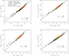 |
Fig. 3. IR-radio correlations. Top-left: 70 μm–1.4 GHz correlation. Top-right: 100 μm–1.4 GHz correlation. Bottom-left: 160 μm–1.4 GHz correlation. Bottom-right: TIR–1.4 GHz correlation. The colored and black symbols show model galaxies. For clarity, the z ∼ 0.5 LIRGs are shown as yellow diamonds in the bottom-right panel. The solid and dotted black lines mark the model linear regression. The gray dots show the observations. |
Basu et al. (2015) studied the radio–TIR correlation in SF galaxies chosen from the PRism MUltiobject Survey up to redshift 1.2 in the XMM-LSS field, employing the technique of image stacking. These authors found an exponent of the TIR–1.4 GHz correlation of α = 1.11 ± 0.04. Bell (2003) assembled a diverse sample of local galaxies from the literature with FUV, optical, IR, and radio luminosities. They found a nearly linear radio–IR correlation. For all galaxy samples except the low-mass and dwarf galaxies we calculated the slopes and offsets of the radio-TIR correlation using an outlier-resistant bisector fit (left panels of Fig. 4). Our model 1.4 GHz luminosities, and especially those of the SF low-mass and dwarf galaxies, are entirely consistent with the results of Bell (2003) and Basu et al. (2015). We conclude that our sample of SF low-mass and dwarf galaxies follows the radio-IR correlation of the more massive SF galaxies.
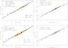 |
Fig. 4. Left panels: TIR–1.4 GHz correlations. The symbols show the model galaxies. Black solid and dotted lines show the model linear regression. Top: Gray solid and dashed lines show the observed linear regression (Basu et al. 2015). Bottom: Orange error bars show data from Bell (2003). Gray solid and dashed lines mark the observed linear regression (Bell 2003). Top-right: SFR–1.4 GHz correlation. Bottom-right: SFR–150 MHz correlation. The colored lines show observed correlations of Wang et al. (2019), Smith et al. (2021), and Gürkan et al. (2018). The pluses mark the model galaxies. The dashed black lines in both panels correspond to outlier-resistant linear bisector fits. |
The resulting correlations between the radio luminosity and the SFR are presented in the right panels of Fig. 4 together with the measured correlations from the literature. The fits yield α = 1.17 ± 0.05 at 1.4 GHz and α = 1.12 ± 0.05 at 150 MHz.
5. Discussion
Our model reproduces the IR, CO, and radio continuum observations of our sample of SF low-mass and dwarf galaxies within a factor of 2 (Sect. 4). In the following, the implications for the CO conversion factor, the CO-dark gas, the thermal fraction of the radio continuum emission, the SF law, and the viscous gas transport will be discussed.
5.1. The CO conversion factor
Since the integrated H2 gas mass and CO emission are explicitly calculated by the model, the integrated CO to H2 conversion factor can be determined. The conversion factor varies between ∼5 and ∼500 M⊙ (K km s−1 pc2)−1 within our sample of low-mass and dwarf galaxies (Fig. 5). As expected, the conversion factor shows a strong dependence on stellar mass and metallicity (Fig. 6). It varies approximately linearly with metallicity: αCO ∝ Z−1.2, very close to what Accurso et al. (2017) found using CO and [C II] observations together with multiphase numerical simulations including radiation transfer and chemical modeling.
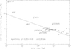 |
Fig. 5. CO(1-0) conversion factor as a function of stellar mass. The solid line corresponds to an outlier-robust linear regression. |
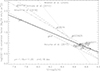 |
Fig. 6. Model CO(1-0) conversion factor as a function of the gas metallicity. The solid line corresponds to an outlier-robust linear regression. The different relations from the literature are labeled. |
Our relation is almost inversely linear, while the exponent found by Madden et al. (2020) is much steeper (−3.4) and those of Schruba et al. (2012), Amorín et al. (2016), and Accurso et al. (2017) are somewhat steeper than our finding. Around solar metallicity all conversion factors, including our model, agree within a factor of 2.
We also calculated the CO conversion factors with twice lower metallicities (Fig. 7). In this case, the model relation is very close to that of Schruba et al. (2012) with a slope of −1.9. The CO conversion factor of DDO 154 increased by a factor of ∼100 when the metallicity was divided by a factor of 2, suggesting a threshold metallicity near 12 + log(O/H = 7.5. Below this limit, virtually all of the CO is photodissociated and the H2 truly CO-dark (no reliable compensation possible via CO-H2 factor). In this 107 M⊙ dwarf galaxy, the CO luminosity abruptly decreases when the metallicity is decreased by a small factor. However, we did not see this kind of behavior in Ho I, which is only two times more massive.
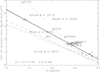 |
Fig. 7. Model with two times lower metallicities than shown in Fig. A.1. Model CO(1-0) conversion factor as a function of the gas metallicity. The solid line corresponds to an outlier-robust linear regression. The different relations from the literature are labeled. |
5.2. CO-dark gas
We can use the model to calculate the CO luminosities without CO photodissociation (see Appendix E). As shown in Fig. 8, without CO photodissociation, the CO luminosities are higher, about a factor of 2 higher than the detected CO luminosities. Most galaxies with CO upper limits (except IC 2574) would have been detected without CO photodissociation.
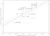 |
Fig. 8. Model CO luminosity without CO photodissociation as a function of the observed CO luminosity. The model including CO photodissociation (Fig. 5) is shown in gray for comparison. |
The CO conversion factors without CO photodissociation are presented in Fig. 9. These can be directly compared to those of Fig. 6. The CO conversion factors of the low-mass NGC galaxies are αCO = 8.5 ± 2.0 M⊙ (K km s−1 pc2)−1, a factor of 2 higher than the Galactic value. Those of the four lowest mass galaxies are more than a factor of 4 higher than the Galactic value.
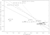 |
Fig. 9. CO(1-0) conversion factor as a function of gas metallicity without CO photodissociation. |
Here we define “CO-dark gas” as being the amount of H2 missed when galactic N(H2)/ICO is used to convert CO brightness to H2 column density. The N(H2)/ICO factor (αCO) increases by a factor of 40 and 10 due to CO photodissociation in DDO 154 and Ho I, respectively. It increases by a factor of 4 in IC 2574 and by a factor of 2 in Ho II and NGC 2403. The increase is ≲50% in the other low-mass galaxies. This mean that ∼98% and ∼90% of the molecular hydrogen mass is CO-dark in DDO 154 and Ho I, respectively. The percentage of CO-dark gas in IC 2574 is ∼75%, that in Ho II and NGC 2403 is ∼50%. Thus, only galaxies with stellar masses ≲109 M⊙ have fractions of CO-dark gas on the level of ≳0.5.
5.3. Intrinsic CO-H2 conversion factor
Running the model without CO photodissociation (but including H2 photodissociation) shows that in slightly subsolar metallicity spirals (e.g., NGC 2403), the photodissociation of CO in the envelopes plays only a small role. The conversion factor αCO decreases from about 8.5 M⊙ (K km s−1 pc2)−1 (corresponding to N(H2)/ICO = 4 × 10²⁰ K km s−1) to 6.0 M⊙ (K km s−1 pc2)−1. However, as the metallicity decreases, the αCO seen without CO photodissociation remains essentially unchanged, whereas the true αCO increases rapidly. Photodissociation is the principal factor controlling αCO: where H2 is not photodissociated, the CO is close to optically thick in the absence of CO photodissociation. The H2 part of clouds in galaxies is intrinsically similar, despite the highly different conditions.
In spiral disks, the UV brightness decreases by more than an order of magnitude between the central regions and R25, whereas the metallicity decreases by a factor of ∼2. Thus, the weak CO emission in outer disks (beyond the effective radius) of solar or slightly subsolar spiral galaxies is not due to CO photodissociation and, instead, to the lower excitation and lower molecular fraction.
5.4. Thermal fraction of the radio continuum emission
The radio continuum SEDs of the low-mass and dwarf galaxies (Fig. C.1) become flatter towards high frequencies because of an increasing fraction of emission of thermal electrons (bremsstrahlung). We calculated the thermal fraction for the different galaxy samples at frequencies between 150 MHz and 30 GHz (Table 2). As expected, the thermal fraction increases from a few percent at 150 MHz to 50–70 % at 30 GHz. Interestingly, the highest thermal fractions are observed in our SF low-mass and dwarf galaxy sample. At 1.4 GHz, the mean thermal fraction is 23%. DDO 154 and IC 2574 have a thermal fraction of 45%, which is consistent with the results of Roychowdhury & Chengalur (2012). These authors found a thermal fraction of ∼50% for their sample of faint dwarf irregular galaxies with typical SFRs of several 10−3 M⊙ yr−1. For our low-mass and dwarf galaxy sample, the thermal fraction is 40% at 5 GHz. It increases to 70% at 30 GHz. Presumably, this is due to the weaker large-scale magnetic field in the smaller galaxies (see also Klein et al. 1984).
Thermal fraction in percent.
5.5. The star formation law
The SF efficiency in local MS galaxies is roughly linear with a gas depletion time of SFE = M(H2)/SFR ∼ 2 Gyr (e.g., Bigiel et al. 2008, 2011). Saintonge et al. (2011a) compared the molecular gas depletion time and global galaxy parameters in a sample of ∼300 local galaxies with 1010 < M* < 1011.5 M⊙. The global molecular gas depletion time was found to vary with stellar mass, stellar surface mass density, light concentration, near-ultraviolet (NUV)-r color, and specifific SFR (sSFR). The strongest dependencies were on seen for the color and sSFR.
The link between model  (SF surface density) and model Σ(H2) (H2 surface density) is presented in Fig. 10. The slope steepens with increasing molecular gas surface density, increasing from linear in local MS galaxies to ∼1.5 for local LIRGs and 0.5 ≤ z ≤ 1.5 MS galaxies to ∼2 for local and high-z starbursts. Part of the steepening could be because at high pressure all of the gas is molecular, increasing the SFR. At high redshift, the galaxies are physically small so the surface densities are high.
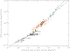 |
Fig. 10. Star formation rate surface density as a function of the molecular gas surface density. The symbols are the same as in Fig. 1. The dashed lines correspond to outlier-robust linear regressions to three subsamples (local MS, intermediate- and high-z MS, and local and high-z starbursts). The dotted lines correspond to exponents of the logarithmic relation of 1, 1.5, and 2, respectively. |
The molecular gas depletion time as a function of the sSFR is shown in Fig. 11 together with the relations determined by Saintonge et al. (2011b) and Huang & Kauffmann (2014). sSFR = Ṁ∗/M∗ and tdep = M(H2)/SFR so the relation (red line) shown is tdep ≈ 103.18 sSFR−0.58. The scatter is 0.12 dex, about half that of Saintonge et al. (2011b) or Huang & Kauffmann (2014). The relation found by Saintonge et al. (2011b) is somewhat steeper (exponent of −0.72), while that of Huang & Kauffmann (2014) is shallower (−0.37) than our model relation. We note that all galaxies except Ho I lie on the model relation. The galaxy sample with the largest scatter is that of the high-z starburst galaxies. It should be noted that the variation in sSFR is very small among spirals (little variation around sSFR ≈ 5 × 10⁻¹¹) and the phase in which a galaxy (necessarily a starburst) has a high sSFR is short. Small galaxies, which generally tend to be chemically young, have much lower stellar masses and (unless they have little or no gas; e.g., local dwarf spheroidals) have higher sSFR and lower gas consumption times.
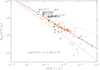 |
Fig. 11. Molecular gas depletion time as a function of the sSFR. The red solid line corresponds to an outlier-robust linear regression to our model galaxies. The symbols are the same as in Fig. 1. The dotted line corresponds to the relation found by Huang & Kauffmann (2014), while the dashed line relates to that of Saintonge et al. (2011b). |
Since the model SF surface density is proportional to the total gas pressure (Fig. A.1 of Vollmer et al. 2025; Ostriker & Kim 2022), a change in regime from vertically non-self-gravitating to self-gravitating gas might lead to the steepening of the SFR correlation with increasing gas surface density. To investigate the influence of vertical self-gravity (0.5 π G Σ2; Eq. (D.8)) on the SF law, we calculated the ratio between the pressure of self-gravitating gas to the total gas pressure,
 (5)
(5)
Since this ratio does not vary significantly between the MS and starburst galaxies and since fselfgrav for local and high-z starburst galaxies are significantly different (Table 3), we conclude that vertical self-gravity does not play an important role in shaping the  –ΣH2 relation. We also calculated our model without vertical gas self-gravity. This led to much higher gas velocity dispersions, approaching the rotation velocities, compared to the models with self-gravity. The resulting logarithmic
  –ΣH2 and SFR–sSFR relations have similar slopes as those of the model with self-gravity, corroborating our conclusion that self-gravity is not responsible for the different slopes of the
  –ΣH2 relation. We argue that it is the combination of a constant mass accretion rate, a SF surface density that is proportional to the gas pressure, a constant Toomre Q parameter, and energy flux conservation (Appendix D) that lead to the observed
  –ΣH2 and SFR–sSFR relations.
Self-gravitating gas disk pressure fraction.
5.6. Radial gas transport
The turbulent viscosity of the gas is given by ν = vturb ldriv. To compare the radial gas accretion rate with gas consumption by SF, we evaluated the SF timescale ( ) and the viscous timescale (tvisc = (R2Ω)″/( − Ω″ν)) at the effective (half-light) radius of each galaxy. Figure 12 shows the model tvisc/t* ratio versus stellar mass for the SF galaxies. We determined tvisc/t* ≲ 1 for all low-mass and dwarf galaxies. Therefore, as argued in Vollmer et al. (2025), we find that viscous gas transport plays a role in SF galaxies with M* ≲ 1010 M⊙.
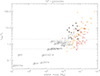 |
Fig. 12. Fraction tvisc/t* as a function of the stellar mass of the model galaxies. Top: SF galaxies. The tvisc/t* fractions of the SF galaxies should thus be taken as lower limits with an uncertainty of a factor of 2 towards higher values. The symbols are the same as in Fig. 1. |
6. Conclusions
We extended the work of Vollmer et al. (2025) related to local and high-z SF and starburst galaxies by adding local SF low-mass and dwarf galaxies. The gas chemistry computed by the Nautilus code depends on the cosmic ray (CR) ionization rate, which was calculated following the analytical model of Pohl (1993) using the local density, magnetic field strength, and radiation field of our analytical model. The injection rate of CR particles was kept proportional to the SFR per volume ( ). The molecular line emission was calculated by RADEX. We then calculated the radio continuum emission of the galaxies following the framework of Vollmer et al. (2022, 2025), Condon & Ransom (2016), and Pacholczyk (1970). For the CR energy loss terms, we used the formalism of Pohl (1993) with the energy loss time scales of Vollmer et al. (2022). The new method has the advantage that the normalization of the CRe density and, as a consequence, of the CR ionization rate is explicitly set within the model framework. The normalization of the CR ionization rate we found for the different galaxy samples is higher by a factor of 3 than the normalization in the solar neighborhood. This means that the mean yield of low-energy CR particles for a given SF surface density is higher by three times in external galaxies than was observed by Voyager I. We found that the thermal fraction of the radio continuum emission of our SF low-mass and dwarf galaxy sample is higher than 40% for frequencies higher than 5 GHz.
The model was applied to seven samples of MS and starburst galaxies (see Sect. 2) at low, intermediate, and high redshifts. Based on the comparison between the model and available observations, we conclude that
-
The model reproduces the IR (Sect. 4.1), CO (Sect. 4.2), and radio continuum (Sect. 4.3) luminosities to within a factor of 2.
-
The model CO-H2 conversion factor, αCO, varies with metallicity as αCO(1 − 0) ∝ 1/Z (Sect. 5.1).
-
The model αCO(1 − 0) varies with stellar mass as M*1/3 (Fig. 5).
-
Photodissociation of CO in cloud envelopes (“CO-dark gas”) is responsible for the variation of αCO with M* and Z. Without CO photodissociation, αCO would remain nearly constant (Sects. 5.2 and 5.3).
-
Star-forming low-mass and dwarf galaxies follow the radio–IR and radio–SFR correlations (Sect. 4.3).
-
The SFR versus H2 mass (expressed as surface densities) is a three-part function that is highly dependent on the subsample (Sect. 5.5).
-
Viscous gas transport is important in galaxies with tvisc ≲ tdepl, which generally corresponds to M* ≲ 1010 M⊙ (Sect. 5.6).
References
- Accurso, G., Saintonge, A., Catinella, B., et al. 2017, MNRAS, 470, 4750 [NASA ADS] [Google Scholar]
- Amorín, R., Muñoz-Tuñón, C., Aguerri, J. A. L., et al. 2016, A&A, 588, A23 [NASA ADS] [CrossRef] [EDP Sciences] [Google Scholar]
- Aniano, G., Draine, B. T., Hunt, L. K., et al. 2020, ApJ, 889, 150 [NASA ADS] [CrossRef] [Google Scholar]
- Basu, A., Wadadekar, Y., Beelen, A., et al. 2015, ApJ, 803, 51 [NASA ADS] [CrossRef] [Google Scholar]
- Beck, R. 2015, A&ARv, 24, 4 [Google Scholar]
- Bell, E. F. 2003, ApJ, 586, 794 [Google Scholar]
- Benson, A., Venkatesan, A., & Shull, J. M. 2013, ApJ, 770, 76 [NASA ADS] [CrossRef] [Google Scholar]
- Bertoldi, F., & McKee, C. F. 1992, ApJ, 395, 140 [NASA ADS] [CrossRef] [Google Scholar]
- Bigiel, F., Leroy, A., Walter, F., et al. 2008, AJ, 136, 2846 [NASA ADS] [CrossRef] [Google Scholar]
- Bigiel, F., Leroy, A. K., Walter, F., et al. 2011, ApJ, 730, L13 [NASA ADS] [CrossRef] [Google Scholar]
- Bolatto, A. D., Wolfire, M., & Leroy, A. K. 2013, ARA&A, 51, 207 [CrossRef] [Google Scholar]
- Condon, J. J. 1992, ARA&A, 30, 575 [Google Scholar]
- Condon, J. J., & Ransom, S. M. 2016, Essential Radio Astronomy (Princeton University Press) [Google Scholar]
- Cormier, D., Madden, S. C., Lebouteiller, V., et al. 2014, A&A, 564, A121 [NASA ADS] [CrossRef] [EDP Sciences] [Google Scholar]
- Cormier, D., Madden, S. C., Lebouteiller, V., et al. 2015, A&A, 578, A53 [CrossRef] [EDP Sciences] [Google Scholar]
- Dale, D. A., Aniano, G., Engelbracht, C. W., et al. 2012, ApJ, 745, 95 [NASA ADS] [CrossRef] [Google Scholar]
- de los Reyes, M. A. C., & Kennicutt, R. C. 2019, ApJ, 872, 16 [NASA ADS] [CrossRef] [Google Scholar]
- Dib, S. 2011, ApJ, 737, L20 [NASA ADS] [CrossRef] [Google Scholar]
- Downes, D., & Solomon, P. M. 1998, ApJ, 507, 615 [NASA ADS] [CrossRef] [Google Scholar]
- Draine, B. T., Dale, D. A., Bendo, G., et al. 2007, ApJ, 663, 866 [NASA ADS] [CrossRef] [Google Scholar]
- Elmegreen, B. G. 1989, ApJ, 338, 178 [NASA ADS] [CrossRef] [Google Scholar]
- Fernandez, E. R., & Shull, J. M. 2011, ApJ, 731, 20 [NASA ADS] [CrossRef] [Google Scholar]
- Fisher, D. B., Bolatto, A. D., White, H., et al. 2019, ApJ, 870, 46 [NASA ADS] [CrossRef] [Google Scholar]
- Freundlich, J., Combes, F., Tacconi, L. J., et al. 2019, A&A, 622, A105 [NASA ADS] [CrossRef] [EDP Sciences] [Google Scholar]
- Gardan, E., Braine, J., Schuster, K. F., et al. 2007, A&A, 473, 91 [NASA ADS] [CrossRef] [EDP Sciences] [Google Scholar]
- Gatto, A., Fraternali, F., Read, J. I., et al. 2013, MNRAS, 433, 2749 [NASA ADS] [CrossRef] [Google Scholar]
- Genzel, R., Tacconi, L. J., Gracia-Carpio, J., et al. 2010, MNRAS, 407, 2091 [NASA ADS] [CrossRef] [Google Scholar]
- Gnedin, N. Y., & Draine, B. T. 2014, ApJ, 795, 37 [Google Scholar]
- Gratier, P., Braine, J., Rodriguez-Fernandez, N. J., et al. 2010, A&A, 512, A68 [NASA ADS] [CrossRef] [EDP Sciences] [Google Scholar]
- Gratier, P., Braine, J., Schuster, K., et al. 2017, A&A, 600, A27 [NASA ADS] [CrossRef] [EDP Sciences] [Google Scholar]
- Gürkan, G., Hardcastle, M. J., Smith, D. J. B., et al. 2018, MNRAS, 475, 3010 [Google Scholar]
- Hersant, F., Wakelam, V., Dutrey, A., Guilloteau, S., & Herbst, E. 2009, A&A, 493, L49 [NASA ADS] [CrossRef] [EDP Sciences] [Google Scholar]
- Huang, M.-L., & Kauffmann, G. 2014, MNRAS, 443, 1329 [NASA ADS] [CrossRef] [Google Scholar]
- Hunt, L. K., García-Burillo, S., Casasola, V., et al. 2015, A&A, 583, A114 [NASA ADS] [CrossRef] [EDP Sciences] [Google Scholar]
- Kelly, B. C. 2007, ApJ, 665, 1489 [Google Scholar]
- Kennicutt, R. C., & De Los Reyes, M. A. C. 2021, ApJ, 908, 61 [NASA ADS] [CrossRef] [Google Scholar]
- Kennicutt, R. C., Calzetti, D., Aniano, G., et al. 2011, PASP, 123, 1347 [Google Scholar]
- Klein, U., Wielebinski, R., & Thuan, T. X. 1984, A&A, 141, 241 [NASA ADS] [Google Scholar]
- Kregel, M., van der Kruit, P. C., & de Grijs, R. 2002, MNRAS, 334, 646 [NASA ADS] [CrossRef] [Google Scholar]
- Krumholz, M. R., McKee, C. F., & Tumlinson, J. 2008, ApJ, 689, 865 [NASA ADS] [CrossRef] [Google Scholar]
- Krumholz, M. R., McKee, C. F., & Tumlinson, J. 2009, ApJ, 693, 216 [NASA ADS] [CrossRef] [Google Scholar]
- Lacki, B. C., Thompson, T. A., & Quataert, E. 2010, ApJ, 717, 1 [Google Scholar]
- Larson, R. B. 1981, MNRAS, 194, 809 [Google Scholar]
- Leitherer, C., Hernandez, S., Lee, J. C., et al. 2016, ApJ, 823, 64 [NASA ADS] [CrossRef] [Google Scholar]
- Leroy, A. K., Walter, F., Brinks, E., et al. 2008, AJ, 136, 2782 [Google Scholar]
- Leroy, A. K., Walter, F., Bigiel, F., et al. 2009, AJ, 137, 4670 [Google Scholar]
- Leroy, A. K., Bolatto, A., Gordon, K., et al. 2011, ApJ, 737, 12 [Google Scholar]
- Leroy, A. K., Rosolowsky, E., Usero, A., et al. 2022, ApJ, 927, 149 [NASA ADS] [CrossRef] [Google Scholar]
- Liszt, H. S. 2007, A&A, 476, 291 [NASA ADS] [CrossRef] [EDP Sciences] [Google Scholar]
- Lizée, T., Vollmer, B., Braine, J., et al. 2022, A&A, 663, A152 [NASA ADS] [CrossRef] [EDP Sciences] [Google Scholar]
- Luo, G., Zhang, Z.-Y., Bisbas, T. G., et al. 2023, ApJ, 946, 91 [NASA ADS] [CrossRef] [Google Scholar]
- Madden, S. C., & Cormier, D. 2019, Dwarf Galaxies: From the Deep Universe to the Present, 344, 240 [Google Scholar]
- Madden, S. C., Rémy-Ruyer, A., Galametz, M., et al. 2013, PASP, 125, 600 [NASA ADS] [CrossRef] [Google Scholar]
- Madden, S. C., Cormier, D., Hony, S., et al. 2020, A&A, 643, A141 [NASA ADS] [CrossRef] [EDP Sciences] [Google Scholar]
- McQuade, K., Calzetti, D., & Kinney, A. L. 1995, ApJS, 97, 331 [Google Scholar]
- Molnár, D. C., Sargent, M. T., Leslie, S., et al. 2021, MNRAS, 504, 118 [CrossRef] [Google Scholar]
- Ostriker, E. C., & Kim, C.-G. 2022, ApJ, 936, 137 [NASA ADS] [CrossRef] [Google Scholar]
- Pacholczyk, A. G. 1970, in Radio astrophysics. Nonthermal processes in galactic and extragalactic sources, (Freeman), Series of Books in Astronomy and Astrophysics [Google Scholar]
- Padoan, P., Nordlund, A., & Jones, B. J. T. 1997, MNRAS, 288, 1 [Google Scholar]
- Pohl, M. 1993, A&A, 270, 91 [NASA ADS] [Google Scholar]
- Ramambason, L., Lebouteiller, V., Madden, S. C., et al. 2024, A&A, 681, A14 [NASA ADS] [CrossRef] [EDP Sciences] [Google Scholar]
- Rémy-Ruyer, A., Madden, S. C., Galliano, F., et al. 2014, A&A, 563, A31 [Google Scholar]
- Rémy-Ruyer, A., Madden, S. C., Galliano, F., et al. 2015, A&A, 582, A121 [Google Scholar]
- Roychowdhury, S., & Chengalur, J. N. 2012, MNRAS, 423, L127 [NASA ADS] [CrossRef] [Google Scholar]
- Roychowdhury, S., Huang, M.-L., Kauffmann, G., et al. 2015, MNRAS, 449, 3700 [NASA ADS] [CrossRef] [Google Scholar]
- Roychowdhury, S., Chengalur, J. N., & Shi, Y. 2017, A&A, 608, A24 [NASA ADS] [CrossRef] [EDP Sciences] [Google Scholar]
- Ruaud, M., Wakelam, V., & Hersant, F. 2016, MNRAS, 459, 3756 [Google Scholar]
- Rujopakarn, W., Rieke, G. H., Weiner, B. J., et al. 2013, ApJ, 767, 73 [NASA ADS] [CrossRef] [Google Scholar]
- Saintonge, A., Kauffmann, G., Kramer, C., et al. 2011a, MNRAS, 415, 32 [NASA ADS] [CrossRef] [Google Scholar]
- Saintonge, A., Kauffmann, G., Wang, J., et al. 2011b, MNRAS, 415, 61 [NASA ADS] [CrossRef] [Google Scholar]
- Schinnerer, E., & Leroy, A. K. 2024, ARA&A, 62, 369 [NASA ADS] [CrossRef] [Google Scholar]
- Schruba, A., Leroy, A. K., Walter, F., et al. 2012, AJ, 143, 138 [NASA ADS] [CrossRef] [Google Scholar]
- Smith, D. J. B., Haskell, P., Gürkan, G., et al. 2021, A&A, 648, A6 [EDP Sciences] [Google Scholar]
- Tacconi, L. J., Neri, R., Genzel, R., et al. 2013, ApJ, 768, 74 [NASA ADS] [CrossRef] [Google Scholar]
- Teich, Y. G., McNichols, A. T., Nims, E., et al. 2016, ApJ, 832, 85 [NASA ADS] [CrossRef] [Google Scholar]
- van der Tak, F. F. S., Black, J. H., Schöier, F. L., Jansen, D. J., & van Dishoeck, E. F. 2007, A&A, 468, 627 [NASA ADS] [CrossRef] [EDP Sciences] [Google Scholar]
- Vieu, T., Gabici, S., Tatischeff, V., et al. 2022, MNRAS, 512, 1275 [NASA ADS] [CrossRef] [Google Scholar]
- Vollmer, B., & Leroy, A. K. 2011, AJ, 141, 24 [Google Scholar]
- Vollmer, B., Gratier, P., Braine, J., et al. 2017, A&A, 602, A51 [NASA ADS] [CrossRef] [EDP Sciences] [Google Scholar]
- Vollmer, B., Soida, M., & Dallant, J. 2022, A&A, 667, A30 [NASA ADS] [CrossRef] [EDP Sciences] [Google Scholar]
- Vollmer, B., Freundlich, J., Gratier, P., et al. 2025, A&A, 693, A267 [NASA ADS] [CrossRef] [EDP Sciences] [Google Scholar]
- Wakelam, V., Herbst, E., Loison, J.-C., et al. 2012, ApJS, 199, 21 [Google Scholar]
- Wang, L., Gao, F., Duncan, K. J., et al. 2019, A&A, 631, A109 [NASA ADS] [CrossRef] [EDP Sciences] [Google Scholar]
- Wolfire, M. G., Hollenbach, D., & McKee, C. F. 2010, ApJ, 716, 1191 [Google Scholar]
- Wyder, T. K., Martin, D. C., Barlow, T. A., et al. 2009, ApJ, 696, 1834 [NASA ADS] [CrossRef] [Google Scholar]
- Yun, M. S., Reddy, N. A., & Condon, J. J. 2001, ApJ, 554, 803 [Google Scholar]
Luo et al. (2023) combined absorption observations of HCO+, and absorption and emission observations of CO to calculate their column densities in the diffuse ISM. The HCO+/CO column density ratio is about constant within a factor of 2–3 for n ≳ 30 cm−3 (Table 2 of Luo et al. 2023).
Appendix A: Gas metallicity
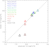 |
Fig. A.1. Model gas metallicity as a function of the observed gas metallicity. The dashed line corresponds to the one-to-one relation. |
Appendix B: IR SEDs
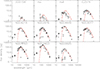 |
Fig. B.1. IR SEDs. Red pluses and solid line: model SED. Dashed red line shows the modified Planck fit for temperature determination. Black crosses show the VizieR photometry. Black boxes show the Herschel data from Dale et al. (2012). The errors bars are given when available from the VizieR tables, but they are often barely visible. |
Appendix C: Radio SEDs
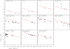 |
Fig. C.1. Radio-continuum SEDs. The model results are shown by red lines. Black crosses: VizieR photometry. The errors bars are shown, if present in the VizieR tables, but often barely visible. |
Appendix D: The model gas disk
In this section and the following, we briefly describe the Vollmer et al. (2017) model with the minor modifications given in Vollmer et al. (2025). The meaning of the different variables is given in Appendix C. Following Vollmer & Leroy (2011) and Vollmer et al. (2021), the SFR per unit volume is given by
 (D.1)
(D.1)
where ΦV is the volume filling factor, ρ is the large-scale density, l and ρl = ρ/ΦV the size and density of selfgravitating clouds, and  the local free-fall time. This prescription leads to an SFR per unit area which is proportional to the gas pressure p = ρvturb2 (Fig. A.1 of Vollmer et al. 2022) as expected if SF is pressure-regulated and feedback-modulated (Ostriker & Kim 2022).
For self-gravitating clouds with a virial parameter of two (Bertoldi & McKee 1992), the turbulent crossing time tturb, cl equals 1.4 times the free-fall time tturb, cl:
 (D.2)
(D.2)
where lcl and vturb, cl are the size and the turbulent 1D velocity dispersion of a single gas cloud, respectively. Following Larson’s law (Larson 1981), we can simplify the expression of the turbulent crossing time:
 (D.3)
(D.3)
where δ is the scaling between the driving length scale and the size of the largest self-gravitating structures, such as δ = ldriv/lcl. The expression for the SFR then becomes
 (D.4)
(D.4)
and  .
.
The SFR density is used to calculate the rate of energy injection by supernovae (SNe):
 (D.5)
(D.5)
where ΔA is the unit surface element of the disk,  and
and  the SF per unit area and unit volume, Σ the total gas surface density, ν the turbulent viscosity, vturb the turbulent velocity of the gas, and the CO disk thickness is assumed to be ldriv. The turbulent viscosity is
  . The energy injection rate is related to the turbulent velocity dispersion and the driving scale of turbulence. These quantities in turn provide estimates of the clumpiness of gas in the disk (i.e., the contrast between local and average density) and the rate at which viscosity moves matter inward. The derived expressions for ΦV and
  are
are
 (D.6)
(D.6)
and
 (D.7)
(D.7)
In the model, the disk scale height is determined unambiguously by the assumption of hydrostatic equilibrium and the turbulent pressure (Elmegreen 1989):
 (D.8)
(D.8)
where  is the stellar vertical velocity dispersion and Σ the surface density of gas and stars. The stellar velocity dispersion is calculated by
  , where the stellar vertical height is taken to be H* = l*/7.3 with l* being the stellar radial scale length (Kregel et al. 2002). We neglect thermal, cosmic ray, and magnetic pressure.
The model relies on several empirical calibrations: the relation between the stellar velocity dispersion and the stellar disk scale length, the relationship between the SFR and the energy injected into the ISM by SNe, and the characteristic time of H2 formation, which is related to the gas metallicity and the gas density. The fraction between the molecular and the total gas mass is governed by the turbulent crossing time  and the molecule formation timescale. In addition, photodissociation of molecules is taken into account.
The model is divided into a large-scale and a small-scale part. The former yields the surface density, turbulent velocity, disk height, and gas viscosity. The latter is relevant for self-gravitating gas clouds  . The non-self-gravitating and self-gravitating clouds obey different scaling relations, which are set by observations. For each gas density, the mass fraction of clouds of this density is characterized by a log-normal probability distribution function and the Mach number (Padoan et al. 1997). The temperatures of the gas clouds are calculated via the equilibrium between turbulent mechanical and cosmic ray heating and gas cooling via CO and H2 line emission. The abundances of the different molecules are determined using the time-dependent gas-grain code Nautilus (Hersant et al. 2009; Ruaud et al. 2016). The dust temperatures are calculated via the equilibrium between heating by the interstellar UV and optical radiation field and cooling via IR emission.
Appendix E: Molecular fraction based on photodissociation
For the determination of the H2 column density of a gas cloud, we take into account (i) photodissociation of H2 molecules and (ii) the influence of the finite cloud lifetime on the H2 formation.
For the photodissociation of H2 molecules, we follow the approach of Krumholz et al. (2008, 2009). These authors solved the idealized problem of determining the location of the atomic-to-molecular transition in a uniform spherical gas cloud bathed in a uniform isotropic dissociating radiation field. It is assumed that the transition from atomic to molecular gas occurs in an infinitely thin shell. The cloud has a constant inner molecular and outer atomic gas density. The inner molecular core and the outer atomic shell are assumed to be in thermal pressure equilibrium. The H2 to H I ratio is
 (E.1)
(E.1)
with  . The H I optical depth is
 (E.2)
(E.2)
with the dimensionless radiation field strength χ, which we set to  . Here, we assume a constant ratio between the inner molecular and outer atomic gas density, which is on the order of 10. For
  and solar metallicity, the transition between a molecular- and atomic-dominated cloud occurs at Σcl ≃ 20 M⊙pc−2. The H2 fraction of the cloud is fH2 = RH2/(1 + RH2). This treatment insures a proper separation of H I and H2 in spiral galaxies, that is, clouds of low density (∼100 cm−3) and low column density (∼1021 cm−2) are fully atomic, whereas clouds of high density, that is, GMCs, (≥1000 cm−3) and high column density (≥1022 cm−2) are fully molecular. In starburst regions (e.g., in ULIRGs), where gas densities and surface densities are much higher, this treatment has no effect, since the gas will be fully molecular.
In a second step, we take into account the molecular fraction due to the finite lifetime of the gas cloud  . The total molecular fraction of a cloud is
  . The molecular fraction due to the finite lifetime
  has the highest influence on fmol at large galactic radii.
We now go from the H2 mass fraction to the CO mass fraction. In an externally irradiated gas cloud, a significant H2 mass may lie outside the CO region, that is, it is dark in the outer regions of the cloud where the gas phase carbon resides in C or C+. In this region, H2 self-shields or is shielded by dust from UV photodissociation, whereas CO is photodissociated. Following Wolfire et al. (2010), the dark gas mass fraction for a cloud of constant density is
 (E.3)
(E.3)
with
 (E.4)
(E.4)
and AV = 2 (Z/Z⊙)Ncl/(1.9 × 1021 cm−2) where Ncl is the H2 column density. The CO mass fraction is then  .
.
All Tables
All Figures
|
Fig. 1. Model TIR luminosity as a function of the observed TIR luminosity. The dotted lines show a factor two above and below the equality. |
| In the text | |
|
Fig. 2. Model CO luminosity as a function of the observed CO luminosity for the SF low-mass and dwarf galaxies. The dotted lines show a factor two above and below the equality. |
| In the text | |
|
Fig. 3. IR-radio correlations. Top-left: 70 μm–1.4 GHz correlation. Top-right: 100 μm–1.4 GHz correlation. Bottom-left: 160 μm–1.4 GHz correlation. Bottom-right: TIR–1.4 GHz correlation. The colored and black symbols show model galaxies. For clarity, the z ∼ 0.5 LIRGs are shown as yellow diamonds in the bottom-right panel. The solid and dotted black lines mark the model linear regression. The gray dots show the observations. |
| In the text | |
|
Fig. 4. Left panels: TIR–1.4 GHz correlations. The symbols show the model galaxies. Black solid and dotted lines show the model linear regression. Top: Gray solid and dashed lines show the observed linear regression (Basu et al. 2015). Bottom: Orange error bars show data from Bell (2003). Gray solid and dashed lines mark the observed linear regression (Bell 2003). Top-right: SFR–1.4 GHz correlation. Bottom-right: SFR–150 MHz correlation. The colored lines show observed correlations of Wang et al. (2019), Smith et al. (2021), and Gürkan et al. (2018). The pluses mark the model galaxies. The dashed black lines in both panels correspond to outlier-resistant linear bisector fits. |
| In the text | |
|
Fig. 5. CO(1-0) conversion factor as a function of stellar mass. The solid line corresponds to an outlier-robust linear regression. |
| In the text | |
|
Fig. 6. Model CO(1-0) conversion factor as a function of the gas metallicity. The solid line corresponds to an outlier-robust linear regression. The different relations from the literature are labeled. |
| In the text | |
|
Fig. 7. Model with two times lower metallicities than shown in Fig. A.1. Model CO(1-0) conversion factor as a function of the gas metallicity. The solid line corresponds to an outlier-robust linear regression. The different relations from the literature are labeled. |
| In the text | |
|
Fig. 8. Model CO luminosity without CO photodissociation as a function of the observed CO luminosity. The model including CO photodissociation (Fig. 5) is shown in gray for comparison. |
| In the text | |
|
Fig. 9. CO(1-0) conversion factor as a function of gas metallicity without CO photodissociation. |
| In the text | |
|
Fig. 10. Star formation rate surface density as a function of the molecular gas surface density. The symbols are the same as in Fig. 1. The dashed lines correspond to outlier-robust linear regressions to three subsamples (local MS, intermediate- and high-z MS, and local and high-z starbursts). The dotted lines correspond to exponents of the logarithmic relation of 1, 1.5, and 2, respectively. |
| In the text | |
|
Fig. 11. Molecular gas depletion time as a function of the sSFR. The red solid line corresponds to an outlier-robust linear regression to our model galaxies. The symbols are the same as in Fig. 1. The dotted line corresponds to the relation found by Huang & Kauffmann (2014), while the dashed line relates to that of Saintonge et al. (2011b). |
| In the text | |
|
Fig. 12. Fraction tvisc/t* as a function of the stellar mass of the model galaxies. Top: SF galaxies. The tvisc/t* fractions of the SF galaxies should thus be taken as lower limits with an uncertainty of a factor of 2 towards higher values. The symbols are the same as in Fig. 1. |
| In the text | |
|
Fig. A.1. Model gas metallicity as a function of the observed gas metallicity. The dashed line corresponds to the one-to-one relation. |
| In the text | |
|
Fig. B.1. IR SEDs. Red pluses and solid line: model SED. Dashed red line shows the modified Planck fit for temperature determination. Black crosses show the VizieR photometry. Black boxes show the Herschel data from Dale et al. (2012). The errors bars are given when available from the VizieR tables, but they are often barely visible. |
| In the text | |
|
Fig. C.1. Radio-continuum SEDs. The model results are shown by red lines. Black crosses: VizieR photometry. The errors bars are shown, if present in the VizieR tables, but often barely visible. |
| In the text | |
Current usage metrics show cumulative count of Article Views (full-text article views including HTML views, PDF and ePub downloads, according to the available data) and Abstracts Views on Vision4Press platform.
Data correspond to usage on the plateform after 2015. The current usage metrics is available 48-96 hours after online publication and is updated daily on week days.
Initial download of the metrics may take a while.