© The Authors 2026

1 Introduction

Interesting scientific problems usually have a long and somewhat complex history. That is also the case of variations in eclipse epochs of binary stars embodied in systems of a higher hierarchy attributed to the finite speed of light. As the center of mass (COM) of the binary periodically moves along the line of sight to the observer, due to its revolution about the global COM of the whole system, epochs of eclipses are either delayed or advanced; this phenomenon is often termed the light-time effect (LITE; though some authors prefer the light-travel-time effect; LTTE). However, even in the simplest of such situations, triple-star systems, the variations in eclipse epochs may arise for several other reasons, including mutual interactions of the components in the binary or gravitational perturbations of the three stars in the system. Separation of the role of these different phenomena proved tricky and required only a sufficiently long series of good-quality photometric and spectroscopic observations.

The origin of the idea concerning the role of LITE in describing inequalities of eclipses of variable stars belongs to Chandler (1888, 1892), who analyzed century-long observations of Algol (β Persei). Although pleased with the concept of the phenomenon, Tisserand (1895) pointed out another solution of the data, which was further supported by analysis of the spectroscopic observations by Curtiss (1908)¹. Nevertheless, the seed remained, and, on the suggestion of Ejnar Hertzsprung (see Hertzsprung 1922), the first formal mathematical analysis of LITE was developed by Woltjer (1922); the method was later extended by Irwin (1952). However, progress in terms of the photometric observations was rather slow. Their available accuracy implied that LITE may be detected for systems of a sufficiently long period, P₂, of the outer orbit, which required long series of data and supportive spectroscopic evidence of the third star in the system. Reviews by Frieboes-Conde & Herczeg (1973) and Mayer (1990) concluded that there were only a handful of stellar systems with an unambiguous detection of LITE.

Things have dramatically changed in the last two decades or so, mainly due to very accurate space-born photometric surveys of the Kepler, CoRoT, and TESS missions. A breathtaking set of multiple stellar systems of all possible geometries and mass regimes was discovered and accurately characterized (e.g., Rappaport et al. 2013; Conroy et al. 2014; Borkovits et al. 2015, 2016; Borkovits 2022). At the same time, the theory of dynamical interactions in triple systems, including their implications for eclipse timing variations, has seen significant improvements (e.g., Borkovits et al. 2003, 2011, 2015; Borkovits 2022). As a result, the portfolio of precise data and accurate tools for their analysis has significantly increased.

In contrast to these huge advances in theoretical description of the eclipse inequalities due to physical interaction between stars in triple systems, the theory of LITE did not see much development in the context of stellar systems for a long time following the Irwin formulation. New ideas came with the first detections of exoplanets using transits of their hosting stars, and especially the first successful observations of inequalities in their periodicity (transit timing variations; e.g., Fabrycky 2010). Since the same space-born photometric surveys furnished the data for transiting exoplanets and eclipsing binaries, stellar astronomers brought the new findings on detailed modeling of light-travel effects to their field as well. For example, Kaplan (2010) considered the asymmetric shift in accurately measured primary and secondary eclipses of white dwarf systems due to the finite speed of light to constrain the stellar masses. The most recent remarkable advancement in LITE modeling was presented by Conroy et al. (2018). Apart from the traditional LITE due to radial motion of the binary with respect to the observer, these authors pointed out that asymmetry in the transverse motion of the two stars in the binary should cause an additional shift in the observed eclipses. They developed a conceptually general formulation of the effect and applied it to several relevant situations, including hierarchical triple systems. Arguing that the effect is maximal for coplanar systems, they focused their analysis on this case. Studying the LITE correction of the same physical essence as Conroy et al. (2018), namely due to the corrected positions of stars at the center of eclipse caused by the finite travel time of light in the binary system, we used a different approach that allowed us to obtain more general and accurate results. In particular, we provide an analytical formulation for a general orbital architecture of triple systems. This helped us to find that the same maximal effect discussed in the coplanar case also occurs in various non-coplanar systems.

In what follows, we consider two refinements of LITE analytical modeling. After briefly introducing notation and reviewing the traditional analysis of LITE in Sect. 2.2, in Sect. 3.1 we provide a detailed analysis of the role of the finite travel time of light in the binary for generally non-coplanar systems. We restrict ourselves to the case of small eccentricity of the binary, but allow an arbitrary eccentricity of the orbit of the third star in the system. In Sect. 3.2, we analyse LITE shift due to mutual gravitational perturbation of the binary orbit and the orbit of the third star. We provide an analytic estimate of the principal effect with periodicity of the outer orbit in the triple. Since we find this LITE correction small, we restricted ourselves to the coplanar geometry of the triple system. Section 4 concludes our findings and provides an outlook for future developments.

2 Preliminaries

We considered a triple star system in 2+1 hierarchy, namely an eclipsing binary accompanied by a third component. The masses of stars in the binary are m₀ and m₁, and m₂, which is that of the third star. We also define M₁ = m₀ + m₁, the total mass of the binary, and M₂ = M₁ + m₂, the total mass of the system. The configuration of the triple is described using the Jacobi system of coordinates, namely r₁, describing the position of star 1 with respect to star 0, and r₂, the position of star 2 with respect to the COM of the binary. The COM of the whole system is assumed at the origin of the inertial system. The vectors r₁ and r₂ are represented using Keplerian orbital elements, either fixed (Sects. 2.2 and 3.1) or osculating (Sect. 3.2). In what follows, we provide results for a general configuration of the triple system using the osculating Keplerian elements of both orbits. We only assume that the eccentricity, e₁, of the binary orbit is small and introduce non-singular variables k₁ = e₁ cos ω₁ and h₁ = e₁ sin ω₁, where ω₁ denotes the argument of pericenter deduced from the tangent plane to the celestial sphere. Note that the generalization to nonzero eccentricity, e₁, is straightforward, although algebraically complex. At this moment, we postponed this extension of the present analysis to future work. The inclinations i₁ of the binary orbit and i₂ of the third star orbit are arbitrary, the former being only constrained by the existence of eclipses.

2.1 Geometric condition of eclipse mean epoch

We adopted a standard frame in which the XY reference plane is tangent to the celestial sphere and the Z axis is directed to the observer. The eclipse epochs are defined by configurations of minimum sky-plane separation of the stars in the binary. Denoting r₁ = (x₁, y₁, z₁)^T in Cartesian coordinates, the epochs of eclipses minimize the function $F=x_1^2+y_1^2$. Adopting the elliptic solution for r₁ and replacing the derivative with respect to time, t, by the derivative with respect to the true anomaly, f₁, the eclipse epochs satisfy $$\frac{d}{dt}(x_1^2+y_1^2)=n_1{\eta }_1{\left(\frac{a_1}{r_1}\right)}^2\frac{d}{d{f}_1}(x_1^2+y_1^2)=0,$$(1)

where n₁ and a₁ denote the mean motion and semimajor axis of the binary orbit and ${\eta }_1=\sqrt{1-e_1^2}$. It is also customary to introduce the argument of latitude ϕ₁ = ω₁ + f₁ and a related auxiliary angle, θ = ϕ₁ − θ_±, where θ₊ = π/2 for primary eclipses and θ₋ = 3π/2 for secondary eclipses². Finally, denoting x = sin θ, the eclipse epochs satisfy (see, e.g., Gimenez & Garcia-Pelayo 1983) $$ℬx=(\mathcal{A}-x)\sqrt{1-x^2},$$(2)

with $$\mathcal{A}=\mp I{k}_1,ℬ=\pm (I+1)h_1,$$(3)

where $$I=\frac{{\cos }^2{i}_1}{{\sin }^2{i}_1},I+1=\frac{1}{{\sin }^2{i}_1}.$$(4)

The upper sign in Eq. (3) corresponds to the primary eclipses, while the lower sign corresponds to the secondary eclipses. Equation (2) has a solution: $$x=\frac{\mathcal{A}}{1+ℬ}+O\left(e_1^4\right),$$(5)

which implies θ = 𝒜 + O (e₁) (obviously, θ or ϕ₁ are defined up to a factor 2πk, where k is an arbitrary integer number). At the epoch of eclipses, $\sin {\varphi }_1^{\pm }=\pm 1+O(e_1^2)$, $\cos {\varphi }_1^{\pm }=I{k}_1+O(e_1^3)$, and at the distance of the two stars in the binary system $a_1\left[1\mp h_1+O(e_1^2)\right]$.

2.2 Light-time effect: Traditional description

Having set the COM of the whole triple system at the origin of the inertial frame, the inertial positions of the three stars are given by $$R_0=-{\mu }_2{r}_2-{\mu }_{-}{r}_1,$$(6) $$R_1=-{\mu }_2{r}_2+{\mu }_{+}{r}_1,$$(7) $$R_2=(1-{\mu }_2)r_2,$$(8)

where µ₋ = m₁/M₁, µ₊ = m₀/M₁ and µ₂ = m₂/M₂ (with the obvious constraint µ₋ + µ₊ = 1). The inertial position of the COM of the binary is given by the first term on the right-hand side of Eqs. (6) and (7).

In this work, we chose the Z = 0 of the global COM as the reference level for LITE³. Denoting parameters of the third-star orbit binary’s eclipses, $r_2^{\pm }$ and ${\varphi }_2^{\pm }$, namely their distance and argument of latitude, the finite speed c of light implies a variation of eclipse epochs, ∆t_±, given by $$c\text{Δ}{t}_{\pm }={\mu }_2{r}_2^2\pm \sin {\varphi }_2^{\pm }\sin i_2-{\mu }_{\pm }{a}_1\left[1\mp h_1+O\left(e_1^2\right)\right]\sin i_1.$$(9)

The first term in Eq. (9) arises from the motion of the binary’s COM along the observer’s line of sight. This is what most of the literature adopts as the LITE (e.g., Hinse et al. 2012; Borkovits et al. 2015, 2025). The second term is due to the motion of the binary components with respect to their COM. This effect is small and is most often neglected. However, it is important to keep it in our formulation, because it combines with the inner component of the time correction discussed in Sect. 3.1.

3 Light-time effect: Fine-tuning

3.1 Light-travel time in the binary system

We now return to the condition set by Eq. (1) for eclipse epochs and its solution outlined in Sect. 2.1. The projected coordinates x₁ and y₁ of the relative vector between the stars in the binary are given by x₁ = ± (R₁ − R₀) · e_X and y₁ = ± (R₁ − R₀) · e_Y, where (e_X, e_Y) are unit vectors defining the plane tangent to the celestial sphere. A fundamental implicit assumption in Sect. 2.1 was that both vectors R₀ and R₁ are given at the same time, t, which is eventually the epoch of the eclipses used in Eq. (1). Because of the finite speed of light, this setup is not precise and needs to be clarified.

We now consider the situation of the primary eclipse at time t such that the star indexed 1 is at R₁(t). In this case, the star indexed 0 is seen at some retarded time t − ∆t, thus $R_0(t-\text{Δ}t)=R_0(t)-{\dot{R}}_0(t)\text{Δ}t+O(\text{Δ}{t}^2)$, where the overdot mean time derivative. The time interval ∆t, which is small enough to neglect its higher powers, is set by the light travel from star 0 to star 1 along the observer’s line of sight; thus, |(R₁(t) − R₀(t − ∆t)) · e_Z| = c∆t. Since velocities of stars in the triple system are small with respect to the speed of light, we may approximate c∆t = |z₁|. Returning to the eclipse condition, the projected x− and y−coordinates of the relative vector in Eq. (1) should now read $x_1^{\prime }=x_1+({\dot{R}}_0\cdot e_X)\text{Δ}t$ and $y_1^{\prime }=y_1+({\dot{R}}_0\cdot e_Y)\text{Δ}t$, with all coordinates given at a common time, t. The eclipse now follows from the minimization of $F^{\prime }=x_1^{\prime 2}+y_1^{\prime 2}$ or $$F^{\prime }=F-\left[2{\mu }_2(x_1{\dot{x}}_2+y_1{\dot{y}}_2)+{\mu }_{-}\frac{dF}{dt}\right]\frac{\left|z_1\right|}{c}.$$(10)

Consider now that the reference eclipse, as given by the approximate solution in Sect. 2.1, occurred at a certain epoch t₊ (i.e., at which F has been minimized). The minimization of F′ in Eq. (10) implies a different but close epoch of t₊ + ∆t₊. In what follows, we determine two contributions of ∆t₊ from the two terms in the bracket on the right-hand side of Eq. (10), starting with the latter –to be denoted $\text{Δ}{t}_{+}^{\text{in}}$, since it depends uniquely on motion of the stars in the binary– and following with the former–to be denoted $\text{Δ}{t}_{+}^{\text{out}}$, since it depends on the transverse motion of the binary COM due to the third star.

We recall that the second term in Eq. (10) is already a small correction, so we can write $$\begin{array}{lll}{\frac{d{F}^{\prime }}{dt}|}_{t_{+}+\text{Δ}{t}_{+}^{\text{in}}}\hfill & =\hfill & {\frac{dF}{dt}|}_{t_{+}+\text{Δ}{t}_{+}^{\text{in}}}-\frac{{\mu }_{-}}{c}\frac{d}{dt}{\left[\left|z_1\right|\frac{dF}{dt}\right]}_{t_{+}}\hfill \\ \hfill & =\hfill & {\frac{d^{2}F}{d{t}^2}|}_{t_{+}}\left[\text{Δ}{t}_{+}^{\text{in}}-\frac{{\mu }_{-}\left|z_1^{+}\right|}{c}\right]+O\left(\text{Δ}{t}_{+}^{{\text{in}}^2}\right)=0,\hfill \end{array}$$(11)

from which it directly follows that $c\text{Δ}{t}_{+}^{\text{in}}={\mu }_{-}\left|z_1^{+}\right|={\mu }_{-}{a}_1\left[1-h_1+O(e_1^2)\right]\sin i_1$. This term combines with the corresponding contribution in the second term in the right-hand side of Eq. (9) to become $c\text{Δ}{t}_{+}^{\text{in}}=a_1({\mu }_{-}-{\mu }_{+})(1-h_1)\sin i_1$.

A more interesting contribution of $\text{Δ}{t}_{+}^{\text{out}}$ arises from the first term in the right-hand side of Eq. (10). Here, we have $${\frac{d{F}^{\prime }}{dt}|}_{t_{+}+\text{Δ}{t}_{+}^{\text{out}}}={\frac{d^{2}F}{d{t}^2}|}_{t_{+}}\text{Δ}{t}_{+}^{\text{out}}-\frac{2{\mu }_2}{c}\frac{d}{dt}{\left[\left|z_1\right|(x_1{\dot{x}}_2+y_1{\dot{y}}_2)\right]}_{t_{+}}=0,$$(12)

implying $$c\text{Δ}{t}_{+}^{\text{out}}=2{\mu }_2\frac{d}{dt}{\left[\left|z_1\right|(x_1{\dot{x}}_2+y_1{\dot{y}}_2)\right]}_{t_{+}}{\left({\frac{d^{2}F}{d{t}^2}|}_{t_{+}}\right)}^{-1}.$$(13)

Given the subtleness of the effect, we restricted ourselves to the limit of the circular orbit of the binary. In this approximation, we have ${d^{2}F/d{t}^2|}_{t_{\pm }}=2n_1^2{a}_1^2{\sin }^2{i}_1+O(e_1)$. Note that $d^{2}F/d{t}^2=2\left({\dot{x}}_1^2+{\dot{y}}_1^2+x_1{\ddot{x}}_2+y_1{\ddot{y}}_2\right)$. If we were to approximate the second derivative of F at eclipse epochs by only the velocity terms and neglecting the contribution of the acceleration terms, we would have ${d^{2}F/d{t}^2|}_{t_{\pm }}\simeq 2n_1^2{a}_1^2$. As a result, the factor sin i₁ in the final formula (16) would change from the denominator to the numerator (as in Conroy et al. 2018).

Evaluating the same effects for the secondary eclipses, we obtained the first contribution $c\text{Δ}{t}_{-}^{\text{in}}={\mu }_{+}\left|z_1^{-}\right|={\mu }_{+}{a}_1\left[1+h_1+O(e_1^2)\right]\sin i_1$, which now adds with the second term in the right-hand side of Eq. (9), making it $c\text{Δ}{t}_{-}^{\text{in}}=a_1({\mu }_{+}-{\mu }_{-})(1+h_1)\sin i_1$. This effect remains of limited importance for stellar systems in which the masses m₀ and m₁ are comparable. More significant is the second correction, now reading as $$c\text{Δ}{t}_{-}^{\text{out}}=-2{\mu }_2\frac{d}{dt}{\left[\left|z_1\right|(x_1{\dot{x}}_2+y_1{\dot{y}}_2)\right]}_{t_{-}}{\left({\frac{d^{2}F}{d{t}^2}|}_{t_{-}}\right)}^{-1}.$$(14)

Altogether, the resulting inner part of the LITE correction for primary and secondary eclipses reads $$c\text{Δ}{t}_{\pm }^{\text{in}}=\mp a_1({\mu }_{+}-{\mu }_{-})(1\mp h_1)\sin i_1,$$(15)

and it requires non-equal-mass binaries (or a star–planet system) to be nonzero. Even then, (i) its amplitude is small, and (ii) if the eccentricity contribution ±h₁ is neglected, it represents merely a constant shift of eclipse timing. However, the opposite sign at primary and secondary eclipses produces their asymmetry, which may be measurable. This effect is well known, applied in exoplanet transit studies (e.g., Fabrycky 2010; Conroy et al. 2018), and has been discussed in Kaplan (2010) in the context of accurate eclipse measurements of binary white dwarfs. In principle, the measured shift may provide a useful constraint on binary-star masses, but in the real world a degeneracy with eccentricity determination (thus the ±h₁ term) would complicate the situation.

The more significant outer component of the LITE corrections of Eqs. (13) and (14) for the primary and secondary eclipses may be expressed using the Keplerian orbital elements of both the binary and the outer orbit and given in a compact form: $$c\text{Δ}{t}_{\pm }^{\text{out}}=\frac{{\mu }_2{a}_2}{{\eta }_2\sin i_1}{\mathcal{Z}}_{\pm },$$(16)

with $$\begin{array}{l}{\mathcal{Z}}_{\pm }=\sin ({\varphi }_2^{\pm }+\text{ΔΩ})+e_2\sin ({\omega }_2+\text{ΔΩ})\hfill \\ -2(\cos {\varphi }_2^{\pm }+e_2\cos {\omega }_2){\sin }^2\frac{i_2}{2}\sin \text{ΔΩ}\hfill \\ -{\eta }_2\cos i_1\frac{n_2}{n_1}{\left(\frac{a_2}{r_2^{\pm }}\right)}^2[\sin ({\varphi }_2^{\pm }+\text{ΔΩ})\hfill \\ -2\sin {\varphi }_2^{\pm }{\sin }^2\frac{i_2}{2}\cos \text{ΔΩ}];\hfill \end{array}$$(17)

∆Ω = Ω₂ − Ω₁ is the difference in nodal longitudes of the two orbits. In the case of a coplanar configuration of the triple system, i₂ = i₁ = i and ∆Ω = 0, Eq. (17) takes a simpler form⁴: $$\begin{array}{l}c\text{Δ}{t}_{\pm }^{\text{out}}=\frac{{\mu }_2{a}_2}{{\eta }_2\sin i}\frac{n_2}{n_1}[\sin {\varphi }_2^{\pm }+e_2\sin {\omega }_2\hfill \\ -{\eta }_2{\cos }^{2}i\frac{n_2}{n_1}{\left(\frac{a_2}{r_2^{\pm }}\right)}^2\sin {\varphi }_2^{\pm }].\hfill \end{array}$$(18)

Note that the general formula (17) is also valid for i₂ = π/2 when both the node Ω₂ and the argument of latitude ${\varphi }_2^{\pm }$ of the outer orbit are undefined. However, the sum $\text{ΔΩ}+{\varphi }_2^{\pm }$ and ∆Ω + ω₂ are well-defined and continuous.

The last term in the bracket of Eq. (17), which is new in the analytical form, is typically small, but the first term represents a contribution to LITE shift, whose magnitude is only a factor n₂/n₁ smaller than the principal effect in Eq. (9). In systems near the stability limit for which the period ratio P₂/P₁ is not too large (e.g., ≤ 20), the correction in Eq. (17) or (18) for coplanar systems may amount to 5–15% of Eq. (9). Also note that the effect is maximum for coplanar geometry (Conroy et al. 2018), but it is easy to verify using Eq. (17) that non-coplanar geometries may not compromise the LITE correction due to the finite light-travel time in the binary system. In fact, even for the case of the outer orbit perpendicular to the orbital plane of the binary, that correction may be exactly the same as for the coplanar geometry depending on the precise architecture of orbits in the triple system. Finally, we point out that our more rigorous analysis considering elliptic motion of both the binary and the third star in the system allowed us to find that the factor sin i₁ in Eqs. (16) and (18) should stand in as a denominator of the multiplicative factor rather than its numerator. This is particularly important for systems where the binary inclination is not too close to 90^◦.

In order to illustrate relevance of the LITE correction due to the finite travel time of light in the binary system, and also to test its accuracy, in Fig. 1 we show results for the well-constrained multiple system ξ Tauri (see, e.g., Nemravová et al. 2016). For the sake of simplicity, we neglected effects of a distant fourth component in the system at this moment and only considered the compact triple core, which consists of an eclipsing binary with a P₁ = 7.146 d period, and a third component with P₂ = 146 d revolution about the COM of the binary. The system is nearly coplanar, with an inclination of i ≃ 87^◦. The binary has a nearly circular orbit, and the outer orbit has an eccentricity of e₂ ≃ 0.2. The best estimates of the three masses are m₀ = 2.23 M_⊙, m₁ = 2 M_⊙, and m₂ = 3.74 M_⊙. The three upper panels of Fig. 1 show results for three different values on the argument of pericenter, ω₂, of the outer orbit. We compare an analytic formulation of LITE correction present in this section (black triangles) with results of a fully fledged numerical analysis that includes effects of light propagation in the system (red and blue stars for primary and secondary eclipses). There is a fairly good agreement of the two results, with the analytic formulation being much less demanding in terms of CPU. The amplitude of the principal LITE component from Eq. (9) is about five minutes, while the amplitude of Eq. (16) is about 15 seconds. In passing, we also note that the eclipse shifts due to the inner effect of Eq. (15) are ≃3.2 s for ξ Tau. Given the formal accuracy of the eclipse timing from TESS photometry, ≲ 5 seconds in the latest sectors, both contributions are relevant.

To further probe the accuracy of the analytic formulation, we show, in the middle and lower panels of Fig. 1, residuals between the numerical simulation and the analytical model. Satisfactorily, their mean value is zero, and no systematic residual signal exceeds ≃0.005 seconds (amounting to ≃0.03% of the LITE correction amplitude, apparently improving accuracy of a similar simulation reported in Conroy et al. 2018, Fig. 11, by more than one order of magnitude). In fact, the residuals are at the level of numerical precision of our simulation⁵. However, it should be pointed out that the optimum accuracy hinges on the assumption of binary’s circular orbit (e₁ = 0). Since the corrections of $\text{Δ}{t}_{\pm }^{\text{out}}$ in Eqs. (16) to (18) do not contain e₁-dependent terms, accuracy would degrade with increasing e₁ value. A generalization of our results that would include e₁-dependent terms is left for future work (our tests show that the loss of accuracy scales linearly with increasing e₁ values for low enough values).

3.1.1 Systemic velocity and higher multiplicity

The formulation given in the previous section assumed an isolated triple system. Here, we briefly discuss the effect of systemic velocity of the triple and the situation when the triple is embedded in a system of higher multiplicity (i.e., accompanied with other, more distant stars on bound orbits).

We next assume that the COM of the triple system is given by R(t), such that at an arbitrary epoch of t = 0 coincides with the origin of an inertial system, and we denote V(t) = dR/dt its velocity. The previous formulation of LITE has to be extended by an obvious component, $$c\text{Δ}{t}_{\pm }=-R_Z(t),$$(20) $$c\text{Δ}{t}_{\pm }^{\text{out}}=\frac{{\mu }_2{a}_2}{\sin i}\frac{{\dot{\omega }}_2}{n_1}\left[\frac{r_2^{\pm }}{a_2}\sin {\varphi }_2^{\pm }-\frac{{\cos }^{2}i}{{\eta }_2}\frac{n_2}{n_1}(\sin {\varphi }_2^{\pm }+e_2\sin {\omega }_2)\right],$$(19)

with an amplitude of about 0.05 s for the ξ Tauri system. When included, the residuals drop to a 0.005 s level, as in Fig. 1.

in Eq. (9), and the correction’s outer term, $$c\text{Δ}{t}_{\pm }^{\text{out}}=\mp 2\frac{d}{dt}{\left[\left|z_1\right|(x_1{\dot{R}}_X+y_1{\dot{R}}_Y)\right]}_{t_{\pm }}{\left({\frac{d^{2}F}{d{t}^2}|}_{t_{\pm }}\right)}^{-1},$$(21)

in Eqs. (13) and (14). The constant systemic velocity of V = V_⊥ + V_∥ e_Z, where V_⊥ is tangent to the sky plane of the triple system provides $$c\text{Δ}{t}_{\pm }^{\text{out}}=\frac{V_{\perp }}{n_1}\frac{\cos \text{ΔΩ}}{\sin i_1},$$(22)

where ∆Ω is the angular distance between V_⊥ and the ascending node of the binary. To illustrate the effect, we considered the ξ Tau system from Fig. 1, where V_∥ ≃ 8.8 km s⁻¹, V_⊥ ≃ 2.0 km s⁻¹, ∆Ω ≃ 160^◦, and n₁a₁ ≃ 180 km s⁻¹ (e.g., Nemravová et al. 2016). The radial component of Eq. (20) accumulates to ∼ 2.6 hr in a decade, but it is merely a constant drift, which is routinely included in data analysis. The transverse part of Eq. (22) amounts to only an ≃0.6 s retardation of eclipses, and it may thus be neglected with currently available observations. This small effect is due to the anomalously small sky-plane velocity V_⊥ of the system. Conroy et al. (2018) analyzed the Gaia Data Release 1 data and found that the distribution of V_⊥ cos Ω has one and two sigma values of ≃29 km s⁻¹ and ≃58 km s⁻¹. Therefore, a time shift in eclipses of up to 10 s is possible. In such a case, if neglected, it could erroneously mis-manifest in the e₁ solution at the ≃0.01 level.

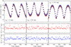Fig. 1 Upper panels: LITE correction due to finite light travel time in the binary system: black triangles are from our analytical model (e.g., $\text{Δ}{t}_{\pm }^{\text{in}}$ and $\text{Δ}{t}_{\pm }^{\text{out}}$ from Eqs. (11) and (13) for primary eclipses), red and blue stars from direct numerical integration of light travel through the system (primary and secondary eclipses). We used parameters of a well constrained multiple system ξ Tauri (e.g., Nemravová et al. 2016) that harbors inner triple system with a distant fourth component (for sake of simplicity the effect of the fourth star was neglected in this example). The triple system is near coplanar with inclination i ≃ 87◦, inner and outer periods P1 = 7.146 d and P2 = 146 d, eccentricities e1 = 0 and e2 = 0.2. The results are shown for three different values of the argument of pericenter of the outer orbit, ω2 = 0 (left panel), ω2 = π/2 (middle panel), and ω2 = 3π/2 (right panel; the present value is ≃10◦ and precesses with a rate ˙ω2 ≃ 2◦ yr−1 due to interaction with the eclipsing binary). The masses are m0 = 2.23 M⊙, m1 = 2 M⊙ and m2 = 3.74 M⊙. Time at abscissa in days covers three revolutions of the outer orbit, LITE on the ordinate in seconds. The mean value of the correction ≃a1/(2c) would combine with the second term on the right hand side of Eq. (9) to be near zero. The P2-periodic variation with an amplitude of ≃15 s is significant and exceeds uncertainty of the TESS photometry. Middle and lower panels: the residuals between the exact numerical simulation and our analytic formulation are shown for primary eclipses by red stars in the middle panel and secondary eclipses by blue stars in the lower panel. Their average value is zero and no signal above ≃0.005 seconds (namely 0.03% of the LITE correction) is observed.

3.2 Coupling with dynamical interaction

Another small correction to the traditional formulation of the LITE arises from the dynamical interaction between the binary and the orbit of the third star in the system. This is because LITE, as described in Sect. 2.2, assumes simple elliptical orbits for the stars in the binary described by r₁ and the third star about their COM described by r₂. In reality, both trajectories are subject to a mutual gravitational interaction in the system.

In this work, we determined the principal correction to LITE due to mutual interaction of stars in the system, leaving a more detailed formulation to future studies. From the multitude of interaction contributions, we considered those with a P₂ periodicity of the outer orbit⁶. We applied a first-order perturbation approach to evaluate the leading correction to the binary’s COM position in the e₁ = 0 and e₂ = 0 limits and assumed a coplanar configuration. The principal LITE contribution in Eq. (9) reads c∆t = −Z, where Z = −µ₂r₂ sin ϕ₂ sin i is the position of the binary’s COM along the line of sight of the observer. By denoting its perturbation by ∆Z, we directly obtained the LITE correction as c∆t^c = −∆Z. We used results from Breiter & Vokrouhlický (2015), the authors of which constructed a Hamiltonian describing secular dynamics of the triple system using Lie–Hori canonical transformation algorithm of short-period term elimination. The associated generating function, S, was useful for our task, as $$\text{Δ}Z=-\{Z;S\}.$$(23)

To keep the work in the lowest order, we also chose the generator, S, describing the quadrupole coupling of the binary and outer orbits in the triple system and restricted it to its part independent of the binary’s eccentricity, e₁. In this approximation, we have $$S=-\frac{2}{3}\frac{C_2}{n_2{\eta }_2^3}(f_2-{\ell }_2+e_2\sin f_2),$$(24)

where $$C_2=\frac{3}{8}\frac{G{m}_2{m}_1^{\prime }}{a_2}{\left(\frac{a_1}{a_2}\right)}^2,$$(25)

$m_1^{\prime }=m_0{m}_1/M_1$ is the reduced mass of the binary, and ℓ₂ is the mean anomaly of the outer orbit. We used Delaunay elements to compute the Poisson bracket {Z; S } in Eq. (23), obtaining a small correction of LITE: $$c\text{Δ}{t}_{\pm }^{\text{c}}={\mu }_2{a}_2\sin i\text{Λ}\left(\sin {\varphi }_2^{\pm }-\frac{1}{6}\cos {\varphi }_2^{\pm }\right),$$(26)

where $$\text{Λ}=\frac{3}{4}\frac{n_2}{n_1}\frac{m_1^{\prime }}{M_2}\sqrt{\frac{M_2{a}_1}{M_1{a}_2}},$$(27)

and in a particular case of equal-mass stars in the binary, we have $$\text{Λ}=\frac{3}{16}{\left(\frac{n_2}{n_1}\right)}^{4/3}{\left(\frac{M_1}{M_2}\right)}^{2/3},$$(28)

or Λ ≃ 0.013 (M₁/M₂)^2/3 for systems near the stability limit period ratio P₂/P₁ ≃ 7.5. For example, the amplitude of LITE correction in Eq. (26) amounts to ≃0.7 s for the ξ Tau system (Λ ≃ 2.2 × 10⁻³). As a result, the effect is truly small, and its relevance is yet to be proven.

4 Conclusions

We developed a new take on the previously published concept of asymmetric transverse velocities of components in a binary for time shifts in exact epochs of their primary and secondary eclipses (Conroy et al. 2018). The finite travel time of light in the binary system itself is the essence of the effect in both Conroy et al. (2018) and our work; therefore, both works extend the classical LITE known in stellar astronomy for a century. We provide a simple analytical formulation valid for generally non-coplanar triple systems containing an eclipsing binary. Although small, the correction to the classical LITE is fully relevant in many systems, with precise photometry provided by space-born surveys available. In Sect. 3.1, we use the multiple stellar system ξ Tauri and an exemplary case. The strength of our result is in its simplicity, which may help to preconstrain model parameters prior to a fully fledged numerical model being applied.

We also analyzed the coupling of LITE with long-period dynamical perturbation of the orbits in the triple system and provided estimates of its contribution to the eclipse timing variation. The corresponding term appears small, at a maximum 0.5–1% of the classical LITE. Nevertheless, advancements in technology may prove to be relevant in the future.

Acknowledgements

The author thanks Petr Zasche and Marek Wolf for useful information on the topic of this paper, and the referee whose suggestions helped to improve its final version. Special thanks belong to Sławek Breiter for his help in computing the Poisson bracket (Eq.(23)). The support of the Czech Science Foundation is acknowledged (grant 25-16507S). This work is dedicated to the memory of Dr. Pavel Mayer, one of the pioneers in rigorously discerning the role of the light time effect in observations of eclipsing binaries.

References

All Figures

Fig. 1 Upper panels: LITE correction due to finite light travel time in the binary system: black triangles are from our analytical model (e.g., $\text{Δ}{t}_{\pm }^{\text{in}}$ and $\text{Δ}{t}_{\pm }^{\text{out}}$ from Eqs. (11) and (13) for primary eclipses), red and blue stars from direct numerical integration of light travel through the system (primary and secondary eclipses). We used parameters of a well constrained multiple system ξ Tauri (e.g., Nemravová et al. 2016) that harbors inner triple system with a distant fourth component (for sake of simplicity the effect of the fourth star was neglected in this example). The triple system is near coplanar with inclination i ≃ 87◦, inner and outer periods P1 = 7.146 d and P2 = 146 d, eccentricities e1 = 0 and e2 = 0.2. The results are shown for three different values of the argument of pericenter of the outer orbit, ω2 = 0 (left panel), ω2 = π/2 (middle panel), and ω2 = 3π/2 (right panel; the present value is ≃10◦ and precesses with a rate ˙ω2 ≃ 2◦ yr−1 due to interaction with the eclipsing binary). The masses are m0 = 2.23 M⊙, m1 = 2 M⊙ and m2 = 3.74 M⊙. Time at abscissa in days covers three revolutions of the outer orbit, LITE on the ordinate in seconds. The mean value of the correction ≃a1/(2c) would combine with the second term on the right hand side of Eq. (9) to be near zero. The P2-periodic variation with an amplitude of ≃15 s is significant and exceeds uncertainty of the TESS photometry. Middle and lower panels: the residuals between the exact numerical simulation and our analytic formulation are shown for primary eclipses by red stars in the middle panel and secondary eclipses by blue stars in the lower panel. Their average value is zero and no signal above ≃0.005 seconds (namely 0.03% of the LITE correction) is observed.

In the text

References

- Borkovits, T. 2022, Galaxies, 10, 9 [NASA ADS] [CrossRef] [Google Scholar]
- Borkovits, T., Érdi, B., Forgács-Dajka, E., & Kovács, T. 2003, A&A, 398, 1091 [NASA ADS] [CrossRef] [EDP Sciences] [Google Scholar]
- Borkovits, T., Csizmadia, S., Forgács-Dajka, E., & Hegedüs, T. 2011, A&A, 528, A53 [NASA ADS] [CrossRef] [EDP Sciences] [Google Scholar]
- Borkovits, T., Rappaport, S., Hajdu, T., & Sztakovics, J. 2015, MNRAS, 448, 946 [NASA ADS] [CrossRef] [Google Scholar]
- Borkovits, T., Hajdu, T., Sztakovics, J., et al. 2016, MNRAS, 455, 4136 [Google Scholar]
- Borkovits, T., Rappaport, S. A., Mitnyan, T., et al. 2025, A&A, 703, A153 [NASA ADS] [CrossRef] [EDP Sciences] [Google Scholar]
- Breiter, S., & Vokrouhlický, D. 2015, MNRAS, 449, 1691 [NASA ADS] [CrossRef] [Google Scholar]
- Chandler, S. C. 1888, AJ, 7, 165 [Google Scholar]
- Chandler, S. C. 1892, AJ, 11, 113 [Google Scholar]
- Conroy, K. E., Prša, A., Stassun, K. G., et al. 2014, AJ, 147, 45 [NASA ADS] [CrossRef] [Google Scholar]
- Conroy, K. E., Prša, A., Horvat, M., & Stassun, K. G. 2018, ApJ, 854, 163 [Google Scholar]
- Curtiss, R. H. 1908, ApJ, 28, 150 [Google Scholar]
- Fabrycky, D. C. 2010, in Exoplanets, ed. S. Seager, 217 [Google Scholar]
- Frieboes-Conde, H., & Herczeg, T. 1973, A&AS, 12, 1 [Google Scholar]
- Frieboes-Conde, H., Herczeg, T., & Høg, E. 1970, A&A, 4, 78 [Google Scholar]
- Gimenez, A., & Garcia-Pelayo, J. M. 1983, Ap & SS, 92, 203 [Google Scholar]
- Hertzsprung, E. 1922, Bull. Astron. Inst. Netherlands, 1, 87 [Google Scholar]
- Hinse, T. C., Goździewski, K., Lee, J. W., Haghighipour, N., & Lee, C.-U. 2012, AJ, 144, 34 [NASA ADS] [CrossRef] [Google Scholar]
- Irwin, J. B. 1952, ApJ, 116, 211 [Google Scholar]
- Kaplan, D. L. 2010, ApJ, 717, L108 [Google Scholar]
- Mayer, P. 1990, Bull. Astron. Inst. Czech., 41, 231 [Google Scholar]
- Nemravová, J. A., Harmanec, P., Brož, M., et al. 2016, A&A, 594, A55 [Google Scholar]
- Rappaport, S., Deck, K., Levine, A., et al. 2013, ApJ, 768, 33 [NASA ADS] [CrossRef] [Google Scholar]
- Tisserand, F. 1895, Bull. Soc. Astron. France Rev. Mens. Astron. Meteor. Phys. Globe, 9, 73 Woltjer, J. 1922, Bull. Astron. Inst. Netherlands, 1, 93 [Google Scholar]
Modern data confirm the LITE contribution to Algol’s eclipse timing variations complemented by a complex mixture of contributions of dynamical origin (e.g., Frieboes-Conde et al. 1970).
The primary eclipse occurs when star 1 eclipses star 0, and the secondary eclipse occurs when star 0 eclipses star 1. In eclipses, θ is a small angle that justifies the subtraction of θ± from the argument of latitude in its definition.
While this choice is arbitrary, we note a difference compared to the work of Conroy et al. (2018), where the reference level for LITE was set at the COM of the binary.
In the case of a coplanar system with retrograde motion of the third component, one has ∆Ω = π and i2 = π − i1. The LITE correction c∆t± is still given by Eq. (18), but now (i) with a reversed sign, and (ii) i = i1 on the right-hand side specifically.
In passing, we note that the simulation shown in Fig. 1 did not account for the observed periastron precession, ˙ω2 ≃ 2◦ yr−1, of the outer orbit. In the case of coplanar configuration, this effect would contribute via an additional LITE correction:
The secular effects, such as periastron precession or inclination variation, may be trivially included in the previous formulation, allowing time dependence of the relevant orbital elements (as an example, see footnote 5).