Online Material
Appendix A: RADEX - construction of a dust model
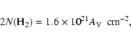
In order to relate the molecular column densities, N(x) of species x, to fractional abundances, X(x) =
![]() ,
a uniform, homogeneous sphere of diameter L =
,
a uniform, homogeneous sphere of diameter L =
![]() is assumed here. The adopted physical diameter of the PDR corresponding to an angular diameter of 120
is assumed here. The adopted physical diameter of the PDR corresponding to an angular diameter of 120
![]() (Sect. 3) at a distance of 910 pc is 0.53 pc. This is assumed to be equal to the line-of-sight depth.
(Sect. 3) at a distance of 910 pc is 0.53 pc. This is assumed to be equal to the line-of-sight depth.
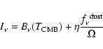
The observed intensity of the continuum is used to estimate the internal radiation field sensed by
the molecules. We construct a simple model of the broad-band spectrum at submm and far-infrared wavelengths in order both to characterise the internal radiation and to estimate the total
column densities of dust and hydrogen. Thronson et al. (1983) measured the far-infrared emission of S140 and found a peak flux density of the order of 104 Jy slightly shortward of ![]() 100
100 ![]() m in a 49
m in a 49
![]() beam. Minchin et al. (1995) presented total broad-band fluxes in a
beam. Minchin et al. (1995) presented total broad-band fluxes in a
![]()
![]()
![]() box. We represent the latter results with a
two-component model of thermal emission by dust over a solid angle of
box. We represent the latter results with a
two-component model of thermal emission by dust over a solid angle of
![]()
![]() 10-7 sr. The main component has a dust temperature
10-7 sr. The main component has a dust temperature
![]() = 40 K and a long-wavelength (
= 40 K and a long-wavelength (
![]() m) form of the opacity law
m) form of the opacity law
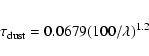
where
where
For the adopted interstellar extinction law and a standard gas/extinction ratio,
the adopted dust model implies
Appendix B: Figures and tables
![\begin{figure}
\par\includegraphics[width=8cm,clip]{0930fig8.eps}
\end{figure}](img151.gif) |
Figure B.1: Odin observations of H218O in the central position. |
| Open with DEXTER | |
![\begin{figure}
\includegraphics[width=8cm,clip]{0930fig9.eps}
\end{figure}](img152.gif) |
Figure B.2:
Rotation diagram of the broad component of 13CO(1-0) with the Onsala 20-m telescope, J = 2-1 and J = 3-2 from Minchin et al. (1993), and J = 5-4 with Odin, producing
|
| Open with DEXTER | |
![\begin{figure}
\includegraphics[width=8cm,clip]{0930fg10.eps}
\end{figure}](img153.gif) |
Figure B.3:
Rotation diagram of the narrow component of 13CO(2-1) and J = 3-2 from Minchin et al. (1993), J = 5-4
with Odin, and J = 6-5 from Graf et al. (1993), producing
|
| Open with DEXTER | |
![\begin{figure}
\par\includegraphics[width=6.9cm,clip]{0930fg11.eps}
\end{figure}](img154.gif) |
Figure B.4: Gaussian fits to 13CO(5-4) at the central position. The widths, amplitudes and centre velocities are 3.2 km s-1 and 8.2 km s-1; 6.610 K and 0.612 K; -7.3 km s-1 and -6.8 km s-1, respectively. |
| Open with DEXTER | |
![\begin{figure}\includegraphics[width=6.9cm,clip]{0930fg12.eps}
\end{figure}](img155.gif) |
Figure B.5:
Gaussian fits to the convolved (to the Odin 126
|
| Open with DEXTER | |
![\begin{figure}\includegraphics[width=6.9cm,clip]{0930fg13.eps}
\end{figure}](img156.gif) |
Figure B.6: Gaussian fits to H2O at the central position. The widths, amplitudes and centre velocities are 3.1 km s-1 and 8.8 km s-1; 416 mK and 213 mK; -7.1 km s-1 and -6.1 km s-1, respectively. |
| Open with DEXTER | |
![\begin{figure}\includegraphics[width=6.9cm,clip]{0930fg14.eps}
\end{figure}](img157.gif) |
Figure B.7: Gaussian fits to NH3 at the central position. The widths, amplitudes and centre velocities are 3.3 km s-1 and 8.5 km s-1; 487 mK and 100 mK; -7.6 km s-1 and -6.4 km s-1, respectively. |
| Open with DEXTER | |
Table B.1: Observed transitions and their parametersa in S140 with the Odin satellite in a five point NE-SW strip.
Table B.2:
13CO Gaussian fitsa. ![]() uses a source size for the PDR (narrow component) of 120
uses a source size for the PDR (narrow component) of 120
![]()
![]() = 2, and a source size for the broad outflow component of 85
= 2, and a source size for the broad outflow component of 85
![]()
![]() = 3.
= 3.
Table B.3:
H2O Gaussian fitsa. ![]() (PDR) uses a source size of 120
(PDR) uses a source size of 120
![]()
![]() = 2, while
= 2, while ![]() (outflow) uses a source size of 85
(outflow) uses a source size of 85
![]()
![]() = 3.
= 3.
Table B.4:
NH3 Gaussian fitsa. ![]() (PDR) uses a source size of 120
(PDR) uses a source size of 120
![]()
![]() = 2, while
= 2, while ![]() (outflow) uses a source size of 85
(outflow) uses a source size of 85
![]()
![]() = 3.
= 3.