Online Material

Appendix A: Selection of the best-fit and the accuracy of the parameter values

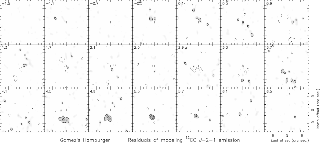$\begin{figure} \rotatebox{270} {\resizebox{8cm}{!}{ \includegraphics{1233fia1.eps} }} \end{figure}$	Figure A.1: Residuals (observations minus synthetic maps) of the ¹²CO J = 2-1 line brightness from our best model fitting for the GoHam disk. The spatial scale and contours are the same as in the observations and predictions, Figs. 1, 6.
Open with DEXTER

A.1 Criteria for acceptable models

The general criterion we chose to select acceptable models was the comparison of the predicted images with the observed ones. Some authors (e.g., Dutrey el al. 2007; Pety et al. 2006; Isella et al. 2007) perform such a comparison in the Fourier transformed plane of the visibilities. The selected model parameters are then those yielding the smallest residuals, after considering `blind' variations of the parameter values. Their method has the advantage of being objective and that uncertainties introduced by the cleaning process are avoided. Other authors (Fuente et al. 2006; Mannings & Sargent 2000,1997) follow, however, a more intuitive approach, comparing directly the images.

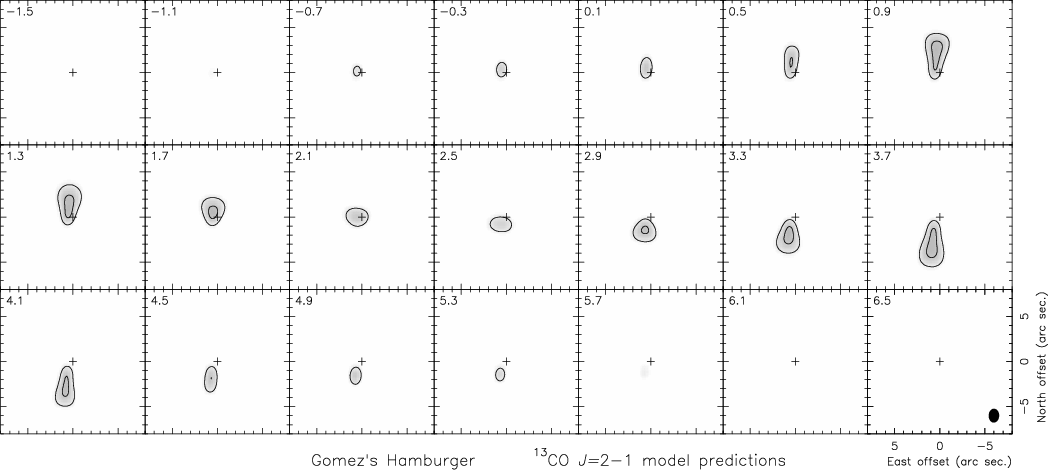$\begin{figure} \rotatebox{270}{\resizebox{8cm}{!}{ \includegraphics{1233fia2.eps} }} \end{figure}$	Figure A.2: Predictions of the ¹³CO J = 2-1 line brightness from our best model fitting for the GoHam disk. The spatial scale and contours are the same as in the observations, Fig. 2.
Open with DEXTER

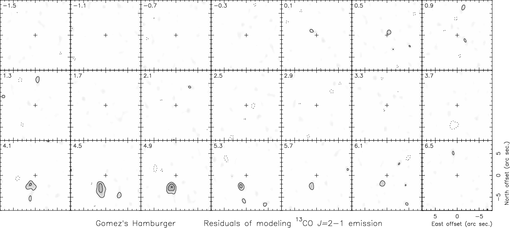$\begin{figure} \rotatebox{270}{\resizebox{8cm}{!}{ \includegraphics{1233fia3.eps} }} \end{figure}$	Figure A.3: Residuals (observations minus synthetic maps) of the ¹³CO J = 2-1 line brightness from our best model fitting for the GoHam disk. The spatial scale and contours are the same as in the observations and predictions, Figs. 2, A.2.
Open with DEXTER

In our case, the high number of free parameters prevents a blind analysis of the resulting residuals for any combination of parameter values, which would imply an exceedingly high amount of calculations. Even the definition of ``free parameter'' in this complex structure is difficult, and it is unclear at what extent we can vary all the disk properties. Even if theoretical constraints on our model parameters are taken into account (see Sect. 3), we continue to have more than 15 (more or less free) model parameters: 5 defining the geometry, 2 for the dynamics, 5 for the temperature, 3 for the density, and finally the ¹²CO/¹³CO/C¹⁷O abundance ratio. It is difficult to decrease such a high number of parameters because of the different components identified in the maps: the hotter and less dense fringes separated from the equator, an outer less dense region, the cold central part of the disk, and the central hotter region.

On the other hand, our procedure allows an intuitive analysis of the relevance of the different parameters. We can infer that some parameters are not so relevant in fitting some observational properties, and that certain observational features are related to only one or two model parameters. For instance, the total size of the disk is selected to match the total extent of the image, which depends weakly on, e.g., the rotational velocity.

It has been argued that in sources comparable in angular size to the telescope resolution, the comparison performed in the image plane is inaccurate. This is untrue in our case, since GoHam occupies an area about 30 square arcseconds, almost a factor of 20 larger than the beam of our ¹²CO J = 2-1 data. The cleaning process always introduces noise, but, besides numerical noise, it is mostly due to uncertainties in the calibration of the complex visibilities, i.e., the true beam shape not being exactly equal to the theoretical beam function (for the uv coverage of the observation). Subtraction of the convolved `clean components' and the subsequent convolution to obtain the final image introduces then spurious features, mainly when the uv sampling is poor. However, such unavoidable uncertainties in the amplitude and phase calibration also appear if the fitting is performed in the uv plane, and the limitation in the dynamic range of the observations due to them applies to both the sky plane and the Fourier transformed plane. On the other hand, we also note that Fourier transformation of the predicted brightness (which must be calculated for a finite grid of points in space coordinates from the standard radiative transfer equation) also introduces numerical noise.

As we see below in actual cases, it is practically impossible to define a single best-fit model in our case, because of the complex data set and model. Instead, we adopt criteria to consider whether a set of parameter values is acceptable and, when they are not satisfied, provide limits to these values. This process will only be detailed for the most representative parameters: radius and width of the disk, central mass (i.e., rotational velocity law), typical densities and temperatures. There is no significant differences among the acceptable models, both in their predictions and in values of the relevant disk properties; one of them was chosen as our best-fit model.

To select the acceptable models, we basically use the comparison of the predictions with the observations of the ¹²CO and ¹³CO J = 2-1 lines, in which S/N and the spatial and spectral resolutions are particularly high. We checked that the predictions for the J = 3-2 lines are also satisfactory. The criteria used to select acceptable models are:

c1) The differential image, i.e., the difference between observed and synthetic velocity channels, must have, in the regions of each channel where emission is present, an rms noise not exceeding $\sim$ 1.5 times that present in adjacent regions with no emission. Those regions, of noise not higher than 1.5 times that found in adjacent ones, are only slightly noticeable in the differential maps.

c2) In the differential J = 2-1 image, the residuals must be smaller than 2 times the spurious contours (due to noise) seen in adjacent regions ( $\sim$ 0.6 Jy/beam, two contours, in our ¹²CO J = 2-1 images), and no residual $\ga$ 0.3 Jy/beam must appear systematically, i.e., in the same spatial offsets for several velocity channels. We note that one can identify noise features more intense than 0.3 Jy/beam in the observed ¹²CO J = 2-1 maps, so residuals not exceeding the above limits are again not clearly different than the observation noise.

These conditions are relaxed for velocities around 4.5-5.5 km s^-1 LSR, which present a strong emission clump with no counterpart in the equivalent blue-shifted emission. This excess cannot be due to opacity or excitation effects, since it is more prominent in the ¹³CO J = 2-1 maps than in the ¹²CO J = 2-1 ones and much more than for ¹²CO J = 3-2. The excess is also clear in the C¹⁷O J = 3-2 maps. The fact that this excess is so remarkable in the less optically thick ¹³CO emission strongly suggests that it is mainly due to the presence of a gas condensation, rotating at about 2.5 km s^-1 at a distance of about $5 \times 10^{15}$ cm from the star. Our model shows axial symmetry and therefore cannot explain this excess; we chose to fit mainly the emission from the rest of the nebula. A tentative model fitting of this feature is presented in A.3, and the consequences and possible origins of the presence of this condensation are discussed in Sect. 4.1.

In Fig. A.1, we present the residuals of our fitting of the ¹²CO J = 2-1 maps. Predictions and residuals for ¹³CO J = 2-1 are shown in Figs. A.2 and A.3. Except for the velocities around 5 km s^-1, the typical rms noise outside the emitting regions is about 0.1-0.11 Jy/beam (slightly less for ¹³CO J = 2-1), and does not exceed 1.5-1.7 Jy/beam in the regions with emission. We see that the largest residuals in the differential images do not reach two contours (noise reaching one level is also seen out of the emitting regions).

Table A.1: Relative range of acceptable values, around those given in Table 1, of the main parameters defining the model disk in Gomez's Hamburger.

Of course, between 4.5 and 5.5 km s^-1, the situation is worse, reflecting the asymmetry in the disk density mentioned above. We can notice some other minor features in the images that are not accounted for by our model. For instance, the ¹³CO line emission at 3.7 km s^-1 is less extended than expected, which is not the case at 4.1 km s^-1. We also note in our ¹³CO maps a weak extent towards the north at about 1.3 km s^-1, but practically at the noise level. In ¹²CO J = 2-1, we see a similar protrusion, but not exactly at the same position. We finally note in some observed panels that the emission from regions close to the star (see, e.g., the ¹³CO J = 2-1 emission at $\sim$ 0.5 km s^-1 and the ¹²CO emission at 3.7 km s^-1) is more extended than the predictions. The width of our disk is given mainly by the equation of hydrostatics (Sect. 3), under the standard theory of massive flaring disks; it is possible that these usual theoretical requirements are not fully satisfied in the innermost regions of the disks, although further analysis of this phenomenon obviously requires higher-quality observations.

A.2 Uncertainty in the fitted parameters

We estimated the uncertainties in derived values of the model parameters by varying the values of each one (while the others remain unchanged) and checking the values for which the above conditions, c1 and c2, were clearly not satisfied. This procedure was completed for the main, most representative parameters, for instance, the disk radius $R_{\rm out}$ , the characteristic density, etc. The results are summarized in Table 1. We also present below some cases in which the uncertainty in the derived parameters requires some discussion.

We did not attempt to consider fully the parameter uncertainties when two or more parameters are allowed to vary. For example, the density range is slightly larger than that given in the table if we allow the temperature also to vary, since both variations are in some way compensated. In general, however, the ranges do not differ very much from our standard uncertainty brackets. The density is mostly fixed by the emission of ¹³CO and that of ¹²CO J = 2-1 from outer regions, while the temperature law is mainly given by the ¹²CO J = 2-1 and J = 3-2 maps.

We note the uncertain determination of the density in the outer disk ( $r \sim R_{\rm out}$ ), which is only given by the ¹²CO emission, since ¹³CO is not detected in this region (see Table A.1). We also recall that the assumption of level population thermalization may be invalid for these diffuse regions, which may imply that the density in them is higher than the values given here, perhaps closer to $3 \times 10^{3}$ cm^-3.

Important problems with the thermalization assumption are unexpected for the relatively high densities of the remaining nebula and the analyzed transitions (Sect. 3). The J=6-5 transition is significantly more sensitive to these effects, due to the relatively high Einstein coefficients of high-J transitions. We also expect underpopulation of the J=6 and J=5 levels in the high-z low-density regions, with $n \sim 10 ^{4}$ cm^-3, leading to 6-5 brightness temperatures of under 10 K. This line would mainly come from this high temperature surface, and we think that this phenomenon is responsible for the non-detection of ¹²CO J=6-5 in our observations. Any further discussion is impossible because of the lack of accurate information about the J=6-5 emission. This relative underpopulation of high-Jlevels in the layers at high absolute values of z may lead to a relative overpopulation of the J=2 level, and therefore to more emission than expected in J = 2-1. This effect could lead to slightly smaller jumps of the temperature, perhaps closer to factor 2.

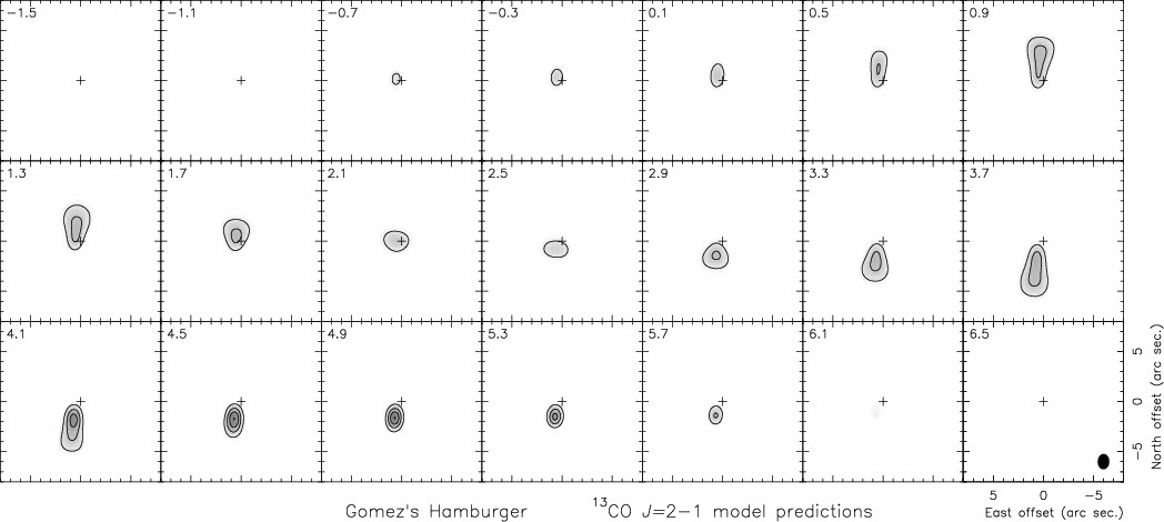$\begin{figure} \rotatebox{270}{\resizebox{8cm}{!}{ \includegraphics{1233fia4.eps} }} \end{figure}$	Figure A.4: Predictions of the ¹³CO J = 2-1 line brightness from our best model fitting for the GoHam disk, including the increase in temperature and density in a southern clump, as described in Appendix A.3. The spatial scale and contours are the same as in the observations, Fig. 2, and our standard model predictions, Fig. A.2.
Open with DEXTER

Some parameter pairs are quite dependent each on other. This is particularly true for the density and CO total abundance, since we assume LTE and then the line opacity depends on the product of the density and the relative abundance. Both parameters can therefore vary freely, provided that their product remains constant. The indetermination is solved assuming a relative ¹²CO abundance of 10^-4. This is also the case for parameters that we have not considered separately in this uncertainty analysis, such as the temperature at a given point, T(R₀), and the slope of the temperature law, $\alpha_T$ ; instead, as mentioned, we discuss the uncertainty in the characteristic temperature. Finally, we note the case of the rotation velocity and the conditions in the hot and dense center of the disk. Strong emission from these regions could mimic the emission of a faster rotating disk in the extreme velocity channels. So, the rotation velocity is mainly determined from the emission extent in the channels at moderate velocities, the emission at the extreme channels depending on both the Keplerian velocity and the emissivity of the central regions. In general, the uncertainty in the parameters defining the inner, denser region ( $r < 2 \times R_{\rm in}$ ) is high, because this clump is not resolved and the number of independent observational constraints is small (as also concluded in Paper I). We can say that an inner region of higher density and temperature is necessary to attain our strong requirements on the fitting quality and that it must be smaller than about 10¹⁶ cm, but we cannot provide details of this region.

The outer hot region, for high values of z, is hardly resolved in our ¹²CO maps. Therefore, we could also reproduce our data assuming that this region is significantly thinner and brighter (in general, hotter) than in our standard model. However, those disk models are less probable than our standard one, since the jump in temperature we found is already quite high (see Sect. 3). Moreover, for very high temperatures in the high-z rim, we should also increase the typical density significantly (to be able to reproduce ¹²CO J = 2-1 data, which, for the assumed dependence of density on z, is only moderately opaque in the high-z regions). This would then imply too low values of X(¹³CO), when attempting to reproduce the ¹³CO J = 2-1 data, leading to improbably high values of X(¹²CO)/X(¹³CO), of significantly over 100. In any case, we note that the properties of this high-z bright rim depend on the relative calibration of the J = 2-1 and J = 3-2 lines; allowing 15% variations in the relative calibrations, we can fit the data with temperature jumps ranging between 2 and 5 (and hot-layer widths that do not differ significantly from our standard value).

A.3 Model (tentative) fitting of the southern brightness maximum

We mentioned that there is a relative maximum in the southern part of the disk that has no counterpart in the north. This maximum is seen in all our maps, but is more prominent in the ¹³CO emission, which is mostly optically thin, as well as in the C¹⁷O line. Therefore, this brightness maximum must be due mainly to an increase in the density of some southern regions, although an increase in temperature is also necessary to explain the excess observed in ¹²CO J = 2-1.

In our standard model analysis, we mostly tried to fit the emission from the rest of the nebula (Sects. 3, A1, A2). Any attempt to fit the emission excess from this southern clump is very uncertain, because of the lack of previous experience in trying to study condensations of this kind, including the lack of theoretical modeling, and because of the poor information contained in our observations, which scarcely resolve its extent.

Nevertheless, we note that this emission excess can be detected over a remarkable range of velocities, between about 4.1 and 5.7 km s^-1 LSR. This means that the emitting condensation cannot be very small, the projected velocity dispersion being caused by gas emission from different distances from the star or from regions showing a significant variation in the velocity projection along the line of sight. In both cases, we expect typical sizes $\sim$ $5 \times 10^{15}$ cm ( $\sim$ 1 $\hbox{$^{\prime\prime}$ }$ for the adopted distance). We can also assume that the condensation occurs in the equatorial disk regions in which ¹³CO J = 2-1 emission originates, because the maximum is so prominent in this line. We have assumed that the emission comes from a region defined by $R_{\rm in} < r < 10^{16}$ cm, and z_s/r < 0.6, where z_s is the distance between a given point and the plane containing the star and perpendicular to the equator that gives the extreme projections for the rotation velocity. We assume that the temperature and density of this region vary with respect to the standard laws assumed for the rest of the nebula.

To explain the (moderate) emission excess found in ¹²CO J = 2-1, we estimate that we must assume an increase in temperature in the southern condensation of a factor $\sim$ 1.5, with respect to our standard laws for nearby regions. Finally, we estimate the excess density in the condensation by comparing the model results with the intensity of ¹³CO J = 2-1. Since the ¹³CO J = 2-1 emission from these inner regions is not fully optically thin and the beam dilution is not negligible, a significant density increase, of a factor 10, is necessary. A total mass increase of about $6 \times 10^{-3}$ $M_{{\odot}}$ is deduced.

The resulting brightness distribution is shown in Fig. A.4. We can see that the brightness excess of ¹³CO J = 2-1 in this southern clump is reasonably well reproduced, but the location of the predicted maximum is slightly closer to the star than the observed one. This cannot be avoided assuming a larger distance from the star for the clump, because then the velocity of the feature would be less positive. The velocity field in this region must then also be disturbed. See discussion on the interpretation of this emission excess in Sect. 4.1.