Online Material
Appendix A: The inverse problem
A.1 The model
As argued in the main text, (Sect. 2.1)
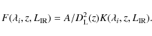
the formal equation relating the number of counts of galaxies
![]() with the flux Sk (within
with the flux Sk (within
![]() )
at wavelength
)
at wavelength ![]() (within
(within
![]() )
to the number of counts of galaxies,
)
to the number of counts of galaxies,
![]() ,
at redshift z (within
,
at redshift z (within
![]() )
and IR luminosity
)
and IR luminosity
![]() (within
(within
![]() )
is given by
)
is given by
![\begin{displaymath}\mathcal{N}(\lambda_i,S_k) = \!\!\int\!\!\!\int\!\delta_{\rm ...
...R}{})\right]\!N(z,L_{\rm IR}){\rm d}{z}~ {\rm d}{L_{\rm IR}} ,
\end{displaymath}](img68.png)
where
 |
(A.2) |
Here,
 |
(A.3) |
where
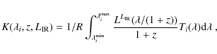
As mentioned in the main text, from the point of view of the conditioning of the inverse problem, it is preferable to reformulate Eq. (A.1)
in terms of
![]() ,
,
![]() and
and
![]() :
:
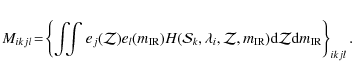
where the kernel of Eq. (A.4) reads
![\begin{displaymath}H(\mathcal{S},\lambda,\mathcal{Z},m_{\rm IR})\equiv 10^{2.5 \...
... D}\!\left[S-F(\lambda,10^\mathcal{Z},10^{m_{\rm IR}})\right]
\end{displaymath}](img80.png)
with
 |
(A.5) |
 |
(A.6) |
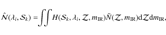
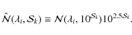
Here we have introduced the Euclidian-normalized number count,
A.2 Discretization
Let us project
![]() onto a complete basis of
onto a complete basis of
![]() functions
functions

of finite (asymptotically zero) support, which are chosen here to be piecewise constant step functions:
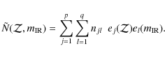
The parameters to fit are the weights njl.
Calling
![]() (the
(the ![]() parameters) and
parameters) and
![]() (the
(the
![]() measurements), Eq. (A.4)
then becomes formally
measurements), Eq. (A.4)
then becomes formally
where M is a
A.3 Penalties
Assuming that the noise in
![]() can be
approximated to be Normal, we can estimate the error between the measured
counts and the non-parametric model by
can be
approximated to be Normal, we can estimate the error between the measured
counts and the non-parametric model by
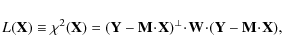
where the weight matrix W is the inverse of the covariance matrix of the data (which is diagonal for uncorrelated noise with diagonal elements equal to one over the data variance). Since we are interested here in a non-parametric inversion, the decomposition in Eq. (A.7) typically involves many more parameters than constraints, such that each parameter controls the shape of the function,
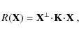
where K is a positive definite matrix, which is chosen so that R in Eq. (A.10) should be non zero when X is strongly varying as a function of its indices. In practice, we use a square Laplacian penalization D2 norm as defined by Eq. (30) of Ocvirk et al. (2006b). Indeed, a Tikhonov penalization does not explicitly enforce smoothness of the solution, and a square gradient penalization favors flat solutions that are unphysical in our problem.
As mentioned in the main text, for a range of redshifts, a direct
measurement,
X0, which can be used as a prior for ![]() ,
is available. We may therefore
add as a supplementary constraint that
,
is available. We may therefore
add as a supplementary constraint that
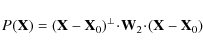
should remain small, where the weight matrix, W2, is the inverse of the covariance matrix of the prior, X0, and should be non zero over the appropriate redshift range. In short, the penalized non-parametric solution of Eq. (A.8) accounting for both penalties is found by minimizing the so-called objective function
where L(X), R(X), and P(X) are the likelihood and regularization terms given by Eqs. (A.9)- (A.11), respectively. The Lagrange multipliers
The minimum of the objective function, Q(X), given by Eq. (A.12) reads formally as
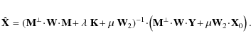
This equation clearly shows that the solution tends towards X0when
Appendix B: Test of robustness
To quantify the confidence level of the inversion technique, we test its robustness. Starting from an arbitrary LF, we produce IR counts in the bands and flux ranges corresponding to the observations from this LF. Then, we add some random Gaussian noise to the simulated counts, using the real uncertainty on the observations as the
The comparison of the input and output LFs is shown in
Fig. B.1. The error on the absolute difference in
![]() is represented in
gray levels and contours. The difference is generally less than
0.4 dex (factor 2.5) in the range where the LF can be constrained from
the observed counts (range of the z-L plane encompassed by the
dashed lines). A noticeable exception is the very low-redshift range
(z<0.1), which corresponds to bright sources. For such large fluxes,
the considerable noise in the observed counts produces large errors on
the recovered LF. At high redshift, recall that the ultra-luminous
population of galaxies appears as rare and very bright objects, in a
flux range where the number counts are poorly known.
is represented in
gray levels and contours. The difference is generally less than
0.4 dex (factor 2.5) in the range where the LF can be constrained from
the observed counts (range of the z-L plane encompassed by the
dashed lines). A noticeable exception is the very low-redshift range
(z<0.1), which corresponds to bright sources. For such large fluxes,
the considerable noise in the observed counts produces large errors on
the recovered LF. At high redshift, recall that the ultra-luminous
population of galaxies appears as rare and very bright objects, in a
flux range where the number counts are poorly known.
![\begin{figure}
\par\includegraphics[width=9cm,clip]{09945f11.ps}
\end{figure}](img106.png) |
Figure B.1:
Estimated robustness of the LF inversion used in
this paper. The relative
difference between the input LF and the recovered LF
(when a realistic noise is added to the corresponding input counts) is larger for
darker parts of the diagram. This difference is relatively small (<0.4 dex)
in the region
of the z-L space effectively constrained by observations: the dotted
and dashed lines correspond to the extreme fluxes considered at 24 |
| Open with DEXTER | |
Appendix C: Model predictions for Herschel
In Sect. 4, we have inverted the known IR counts to obtain constraints on the evolving total IR LF. We have seen that the LF obtained through this inversion is realistic and matches most of the recent observations (counts, CIRB, Mid-IR LF at low redshift). Then, in Sect. 5.2, we have shown how we can measure directly a part of this LF with a good confidence and that the LF resulting from the inversion is in good agreement with this solid measurement, validating the LF obtained by this empirical modeling approach. In this section, we use the median LF obtained from the inversions to predict some counts which should be observed with future observations in the FIR with Herschel or SCUBA2.
At the time of publication, several new facilities
are in preparation to observe the Universe in the far-IR to sub-mm
regimes. The differential counts (normalized to Euclidean) at
wavelengths ranging from 16 to 850 ![]() m, which we derived from the
inversion technique, are presented in Fig. C.3. The
separation of the contribution of local, intermediate, and distant
galaxies in different colors illustrates the expected trend that
larger wavelengths are sensitive to higher redshifts, hence the relative
complementarity of all IR wavelengths. There will be a bias towards
more luminous and distant objects with increasing wavelength,
illustrated here for the Herschel passbands (see
Fig. C.4), but this may be used to pre-select the most
distant candidates expected to be detected only at the largest
wavelengths. In the following, we discuss the predictions of the
inversion technique for those instruments, as well as their respective
confusion limits, which is the main limitation of far-IR extragalactic
surveys.
m, which we derived from the
inversion technique, are presented in Fig. C.3. The
separation of the contribution of local, intermediate, and distant
galaxies in different colors illustrates the expected trend that
larger wavelengths are sensitive to higher redshifts, hence the relative
complementarity of all IR wavelengths. There will be a bias towards
more luminous and distant objects with increasing wavelength,
illustrated here for the Herschel passbands (see
Fig. C.4), but this may be used to pre-select the most
distant candidates expected to be detected only at the largest
wavelengths. In the following, we discuss the predictions of the
inversion technique for those instruments, as well as their respective
confusion limits, which is the main limitation of far-IR extragalactic
surveys.
The ESA satellite Herschel is scheduled to be launched within the next
year, while the next-generation IR astronomical satellite of the
Japanese space agency, SPICA, is scheduled for 2010, with a
contribution by ESA under discussion, including a mid-IR imager named
SAFARI. Both telescopes share the same diameter of 3.5 m, but
the lower telescope temperature of SPICA, combined with projected
competitive sensitivities, will make it possible to reach confusion
around 70 ![]() m (where Herschel is limited by integration time). The
5
m (where Herschel is limited by integration time). The
5![]() -1hour limits of the instruments SAFARI onboard SPICA
(50
-1hour limits of the instruments SAFARI onboard SPICA
(50 ![]() Jy, 33-210
Jy, 33-210 ![]() m, dashed line), PACS (3mJy,
55-210
m, dashed line), PACS (3mJy,
55-210 ![]() m, light blue line) and SPIRE (2 mJy, 200-670
m, light blue line) and SPIRE (2 mJy, 200-670 ![]() m,
blue line) onboard Herschel are compared in Fig. C.1
to the confusion limits that we derive from the best-fit model of the
inversion, at all wavelengths between 30 and 850
m,
blue line) onboard Herschel are compared in Fig. C.1
to the confusion limits that we derive from the best-fit model of the
inversion, at all wavelengths between 30 and 850 ![]() m, assuming the
the confusion limit definition given below.
m, assuming the
the confusion limit definition given below.
![\begin{figure}
\par\includegraphics[width=9cm,clip]{09945f12.ps}
\end{figure}](img107.png) |
Figure C.1:
Confusion limit for a 3.5 m telescope. The
5 |
| Open with DEXTER | |
The definition of the confusion limit is not trivial, in particular because it depends on the level of clustering of galaxies; the optimum way to define it would be to perform simulations to compute the photometric error as a function of flux density, and then decide that the confusion limit is e.g. the depth above which 68% of the detected sources are measured with a photometric accuracy better than 20%. In the following, we only consider a simpler approach that involves computing the two sources of confusion that were discussed in Dole et al. (2003):
- the photometric confusion noise: the noise produced by sources fainter than the detection threshold. The photometric criterion corresponds to the requirement that sources are detected with an S/N(photometric) > 5;
- the fraction of blended sources: a requirement for the quality of
the catalog of sources will be that less than N % of the sources
are closer than 0.8
 FWHM, i.e. close enough to not be
separated.
FWHM, i.e. close enough to not be
separated.
![\begin{figure}
\par\includegraphics[width=8.7cm,clip]{09945f13.ps}
\end{figure}](img112.png) |
Figure C.2:
Detection limits for confusion limited surveys from 70 to
850 |
| Open with DEXTER | |
Table C.1: Fraction of the CIRB resolved by confusion-limited Herschel surveys.
We note that the confusion limit for a 3.5 m-class telescope, such as Herschel, is ten times more than the depth it can reach in one hour (5
![\begin{figure}
\par\includegraphics[width=16.5cm,clip]{09945f14.ps}
\end{figure}](img115.png) |
Figure C.3:
Counts predicted from the inversion in the far-infrared and sub-mm (solid line). The counts are
decomposed in redshift bins (blue = z<0.5; green = 0.5<z<1.5;
orange = 1.5<z<2.5; red = z>2.5). The oblique dashed line corresponds to
the limit in statistics due to the smallness of a field like GOODS
North+South or 0.07 square degrees: less than 2 galaxies per
flux bin of width
|
| Open with DEXTER | |
![\begin{figure}
\par\includegraphics[width=16.6cm,clip]{09945f15.ps}
\end{figure}](img116.png) |
Figure C.4:
Differential counts predicted from the non-parametric
inversion for future Herschel observations: PACS 100 |
| Open with DEXTER | |
For comparison, we also illustrated the ground-based capacity of
ARTEMIS built by CEA-Saclay which will operate at the ESO 12
m-telescope facility APEX (Atacama Pathfinder EXperiment) at 200, 350
and 450 ![]() m and SCUBA-2 that will operate at the 15 m telescope
JCMT at 450 and 850
m and SCUBA-2 that will operate at the 15 m telescope
JCMT at 450 and 850 ![]() m. To avoid confusion between all
instruments, we only show the average wavelength 400
m. To avoid confusion between all
instruments, we only show the average wavelength 400 ![]() m for a 12
m-class telescope and 850
m for a 12
m-class telescope and 850 ![]() m for a 15 m-class telescope
(Fig. C.1). Although the confusion limit in the
850
m for a 15 m-class telescope
(Fig. C.1). Although the confusion limit in the
850 ![]() m passband is ten times below that of Herschel at the
longest wavelengths, this band is not competitive with the
m passband is ten times below that of Herschel at the
longest wavelengths, this band is not competitive with the
![]() 400
400 ![]() m one, which should be priorities for ARTEMIS and
SCUBA-2 for the study of distant galaxies, or with the 70 and
100
m one, which should be priorities for ARTEMIS and
SCUBA-2 for the study of distant galaxies, or with the 70 and
100 ![]() m ones for a 3.5 m space experiment such as SPICA and
Herschel, for redshifts below
m ones for a 3.5 m space experiment such as SPICA and
Herschel, for redshifts below ![]() .
We also note that only in
these two passbands will the cosmic IR background be resolved with
these future experiments (see Table C.1), which suggests
that a larger telescope size should be considered for a future
experiment to observe the far IR Universe above 100
.
We also note that only in
these two passbands will the cosmic IR background be resolved with
these future experiments (see Table C.1), which suggests
that a larger telescope size should be considered for a future
experiment to observe the far IR Universe above 100 ![]() m and below
the wavelength domain of ALMA. We did not mention here ALMA since it
will not be affected by these confusion issue: due to its very
good spatial resolution, it will be limited to either small ultradeep
survey, hence missing rare objects or follow-ups of fields observed
with single dish instruments, e.g. ARTEMIS. Finally, the JWST that
will operate in the mid IR will be a very powerful instrument for probing
the faintest star-forming galaxies in the distant Universe, but
predictions are difficult to produce at the present stage since it has
already been found that extrapolations from the mid to far IR become less
robust already at
m and below
the wavelength domain of ALMA. We did not mention here ALMA since it
will not be affected by these confusion issue: due to its very
good spatial resolution, it will be limited to either small ultradeep
survey, hence missing rare objects or follow-ups of fields observed
with single dish instruments, e.g. ARTEMIS. Finally, the JWST that
will operate in the mid IR will be a very powerful instrument for probing
the faintest star-forming galaxies in the distant Universe, but
predictions are difficult to produce at the present stage since it has
already been found that extrapolations from the mid to far IR become less
robust already at ![]() (e.g. Papovich et al. 2007; Pope et al. 2008; Daddi et al. 2007b).
(e.g. Papovich et al. 2007; Pope et al. 2008; Daddi et al. 2007b).