| Issue |
A&A
Volume 512, March-April 2010
|
|
|---|---|---|
| Article Number | A50 | |
| Number of page(s) | 6 | |
| Section | Interstellar and circumstellar matter | |
| DOI | https://doi.org/10.1051/0004-6361/200912872 | |
| Published online | 31 March 2010 | |
X-ray temperatures and their radial distributions from winds of O-type supergiants: the effects of clumps
J. H. Guo1,2
1 - National Astronomical Observatories/Yunnan Observatory, Chinese
Academy of Science, PR China
2 - Key Laboratory for the Structure and Evolution of Celestial
Objects, Chinese Academy of Sciences, PR China
Received 13 July 2009 / Accepted 15 December 2009
Abstract
Context. Based on the multiphase hydrodynamical
flows and the clump model, a two-fluid model of the
O stars ![]() Ori A
and
Ori A
and ![]() Pup
is investigated, in which the flow is described by a set of
two components.
Pup
is investigated, in which the flow is described by a set of
two components.
Aims. I investigate the influence of clumps on the
production of X-ray and derive wind parameters from a comparison with
the X-ray temperature distributions in the wind of O-type supergiants.
Methods. The velocity structure of the clump is
assumed to be beta law, thus the transonic velocity structure of the
ambient wind can be attained via the shooting method.
Results. The mass, filling factor, and velocity
structure of the clump are very sensitive to the post-shock
temperatures. I find that the filling factor must be about
0.01 for fitting the observed X-ray temperatures. The mass of the clump
cannot be smaller than 1018 g.
A clump carries about ![]() and
and ![]() for
for ![]() Ori A
and
Ori A
and ![]() Pup,
respectively. The model with the exponent of clump velocity
Pup,
respectively. The model with the exponent of clump velocity ![]() for O-type supergiants fits the observations better than one with the
exponent
for O-type supergiants fits the observations better than one with the
exponent ![]() .
.
Conclusions. These results indicate that the forward
shock scenario can explain the X-ray emission, except for the hottest
X-ray lines for O-type supergiants. Theoretical and observable evidence
shows that a low velocity law should be applied to O-type supergiants.
Key words: stars: early type - stars:
individual: ![]() Ori A - stars: individual:
Ori A - stars: individual: ![]() Pup - stars: winds, outflows - X-ray: stars
Pup - stars: winds, outflows - X-ray: stars
1 Introduction
Stellar winds have a strong effect on the evolution of massive stars. Hot stars of spectral O and B have been observed with X-ray emission. Most of the X-ray emission with temperatures of several million degrees from early-type stars appears to originate in their winds (Waldron & Cassinelli 2000, 2007). Solar-type coronal emission was first assumed to explain X-ray emission (Cassinelli & Olson 1979), but the observations did not show the expected large attenuation by the cold winds in the soft X-ray band. The X-ray emissions in normal OB stars are generally explained in terms of shock heating of the supersonic, radiation-driven winds (Lucy & White 1980; Lucy 1982; Cohen et al. 2006). Shocks are distributed throughout their winds and are most likely formed from instabilities of line-driven flow (Lucy & Solomon 1970; Owicki et al. 1988). An important implication of line-driven flow instabilities suggests that the outer winds of OB stars develop extensive structure that is a mixture of rarefied regions and dense ``clumps'' (Feldmeier et al. 1997a; Owocki & Puls 1999), which are typically an order of magnitude denser than the ambient wind.
With the launching of Chandra and XMM-Newton,
high-resolution X-ray emission lines have been detected.
By analyzing their profiles, a direct constraint is available
to the wind-shock model. Much research has shown that the hot, X-ray
emitting plasma is distributed throughout winds (Kramer et al.
2003; Leutenegger et al. 2006a;
Cohen et al. 2006).
The locations and temperatures of the X-ray sources have been measured
in terms of the high-resolution X-ray emission lines (Waldron &
Cassinelli 2000,
2007; Cohen
et al. 2003).
Waldron (2005)
shows that the X-ray temperature distributions decline outward through
the
winds for OB supergiants. Such steady decrease outward from
10 MK (even higher) to 2 MK does not seem
predicted by shock models. Moreover, Waldron & Cassinelli (2007) find that the
X-ray
temperatures of supergiants show a tight correlation with radii. They
find a one-to-one correspondence between
![]() and their associated X-ray continuum optical depth unity radii (
and their associated X-ray continuum optical depth unity radii (
![]() )
when the traditional mass-loss rates were adopted, and explain this as
density dependence. The detailed hydrodynamic numerical simulation
predicted that the winds are permeated by forward and reverse shocks
(Feldmeier et al. 1997a;
Owocki & Puls 1999;
Runacres & Owocki 2002).
A high temperature may be created at low radii if photospheric
turbulence is included.
)
when the traditional mass-loss rates were adopted, and explain this as
density dependence. The detailed hydrodynamic numerical simulation
predicted that the winds are permeated by forward and reverse shocks
(Feldmeier et al. 1997a;
Owocki & Puls 1999;
Runacres & Owocki 2002).
A high temperature may be created at low radii if photospheric
turbulence is included.
Lucy & White (1980)
developed a phenomenological model to explain the X-ray emission in
which the wind is described in terms of a two-component structure,
where one is for the dense clumps and the other for the interclump gas.
This model assumes that clumps are driven by a radiative force while
the ambient gas is pushed along by the drag of these blobs. Therefore,
there are a lot of strong forward shocks in their model. The model can
account for the X-ray luminosity of ![]() Puppis, but fails
for B-type star
Puppis, but fails
for B-type star ![]() Scorpii.
(In fact, Lucy & White did not consider the effect of
clump on the mass-loss rate, which could result in a smaller
attenuation for X-ray luminosity.) An alternative situation is
considered by Howk et al. (2000).
In their model, the clumps move outward(inward) with a
velocity below that of the ambient wind. Thus, a higher
relative velocity can be attained when these clumps fall back towards
the star, producing higher X-ray temperatures. This can explain the
hard X-ray emission in
Scorpii.
(In fact, Lucy & White did not consider the effect of
clump on the mass-loss rate, which could result in a smaller
attenuation for X-ray luminosity.) An alternative situation is
considered by Howk et al. (2000).
In their model, the clumps move outward(inward) with a
velocity below that of the ambient wind. Thus, a higher
relative velocity can be attained when these clumps fall back towards
the star, producing higher X-ray temperatures. This can explain the
hard X-ray emission in ![]() Scorpii.
Scorpii.
The previous studies by Lucy & White (1980) seem to be supported in part by the following facts. First, numerical simulations of the line-driven flow show that the most of flow is composed of``clump'' separated by an almost void interclump medium. Second, the nonlinear interaction from clump collisions result little net velocity-density correlation, which suggests that there is a roughly equal mixture of forward and reverse shocks in the outer wind (Runacres & Owocki 2002).
The main aim of this paper is to investigate the X-ray
temperatures and locations of two O stars ![]() Ori
and
Ori
and ![]() Pup.
I have chosen to use a basic shock model, namely, the forward
shock model. Hydrodynamic simulation predicts that there are reverse
shocks in the inner region of the wind. Thus, a full picture
of shocks in the winds should include both forward and reverse shocks.
However, it is still useful to consider the assumption of
forward shock. First, the X-ray temperature distributions
depend on the square of the relative velocity so that it is difficult
to distinguish the forward with reverse shock from the observed X-ray
temperatures. Second, the
density contrast between the clump and interclump medium is high, which
is supported by both observations and hydrodynamic simulations (Bouret
et al. 2003,
2005; Fullerton
et al. 2006;
Feldmeier et al. 1997a).
The interclump medium is almost void so the
velocity law determined from observations should be the effect of
clumps. Those observations show that the velocity structure of clump is
consistent with the theoretic prediction. Thus, it is not
unreasonable to assume that clumps are driven by radiative force (Thus,
a
Pup.
I have chosen to use a basic shock model, namely, the forward
shock model. Hydrodynamic simulation predicts that there are reverse
shocks in the inner region of the wind. Thus, a full picture
of shocks in the winds should include both forward and reverse shocks.
However, it is still useful to consider the assumption of
forward shock. First, the X-ray temperature distributions
depend on the square of the relative velocity so that it is difficult
to distinguish the forward with reverse shock from the observed X-ray
temperatures. Second, the
density contrast between the clump and interclump medium is high, which
is supported by both observations and hydrodynamic simulations (Bouret
et al. 2003,
2005; Fullerton
et al. 2006;
Feldmeier et al. 1997a).
The interclump medium is almost void so the
velocity law determined from observations should be the effect of
clumps. Those observations show that the velocity structure of clump is
consistent with the theoretic prediction. Thus, it is not
unreasonable to assume that clumps are driven by radiative force (Thus,
a ![]() velocity
law is used.). On the assumption that the clumps move outward with a
velocity below that of the ambient
wind, the motion of clump depends on the drag force of gas. Howk
et al. (2000)
show that the drag force is proportional to the density of the
interclump medium and is inversely proportional to
velocity
law is used.). On the assumption that the clumps move outward with a
velocity below that of the ambient
wind, the motion of clump depends on the drag force of gas. Howk
et al. (2000)
show that the drag force is proportional to the density of the
interclump medium and is inversely proportional to
![]() .
A direct consequence is that the dense clump could fall back
toward the star or move outward with a low velocity, which is not
supported by the observations of O-type supergiants.
And third, by fitting the observed X-ray temperature
distributions, we can determine the extent to which the applying
forward shock model for O-type supergiants may explain the X-ray
temperatures of observations.
.
A direct consequence is that the dense clump could fall back
toward the star or move outward with a low velocity, which is not
supported by the observations of O-type supergiants.
And third, by fitting the observed X-ray temperature
distributions, we can determine the extent to which the applying
forward shock model for O-type supergiants may explain the X-ray
temperatures of observations.
On the assumption that the velocity of the clump is calculated
using a ![]() velocity
law throughout the wind (Sect. 2.1), which results in a low
relative velocity near the star, the model cannot predict a very high
temperature near the star. However, 107 K
temperatures is observed by Waldron & Cassinelli (2007) and predicted
by hydrodynamic simulations. A suitable complement for this
model is to include reverse shocks or magnetic confinement in the inner
wind.
Cassinelli et al. (2008)
suggest that the bow shocks can be produced when the stellar wind
impacts on the clumps. Their results show that the temperature
distribution is a function of the impact parameter for an adiabatic bow
shock and that a high temperature can be produced at the apex of the
shock. In this paper, I only discuss the
forward-shock model. A full description of the forward and
reverse shocks (magnetic confinement)is beyond the scope of
this paper.
velocity
law throughout the wind (Sect. 2.1), which results in a low
relative velocity near the star, the model cannot predict a very high
temperature near the star. However, 107 K
temperatures is observed by Waldron & Cassinelli (2007) and predicted
by hydrodynamic simulations. A suitable complement for this
model is to include reverse shocks or magnetic confinement in the inner
wind.
Cassinelli et al. (2008)
suggest that the bow shocks can be produced when the stellar wind
impacts on the clumps. Their results show that the temperature
distribution is a function of the impact parameter for an adiabatic bow
shock and that a high temperature can be produced at the apex of the
shock. In this paper, I only discuss the
forward-shock model. A full description of the forward and
reverse shocks (magnetic confinement)is beyond the scope of
this paper.
On the assumption of forward shocks, the radiation from stars exerting on the ambient gas is weak because it must first penetrate those clumps. The motion of the ambient gas is mainly controlled by friction between the clumps and the ambient gas. Therefore the main component of the mass loss is more likely clumped and those clumps embedded in smooth gas. The stellar continuum radiation in spectral lines force the clumps to flow away from the star. Lucy & White (1980) solved the two-phase equations of clumps and interclump media; however, they assumed an arbitrary initial value condition. In this model I complement the calculation with a critical transonic solution that yields subsonic velocity at the base of the wind and increases with the critical point outward (also see Guo 2008). Therefore, this paper represents a natural extension of the previous studies by Lucy & White (1980).
The hydrodynamic equations are present in Sect. 2.1.
I briefly discuss the numerical method in Sect. 2.2.
In Sect. 3 I provide a summary of X-ray observations
for ![]() Ori A
and
Ori A
and ![]() Pup.
The numerical results are shown in Sect. 4 and discussed
in Sect. 5, and in Sect. 6 I draw
the conclusions.
Pup.
The numerical results are shown in Sect. 4 and discussed
in Sect. 5, and in Sect. 6 I draw
the conclusions.
2 The model
2.1 Construction of equations
For the multiphase hydrodynamical flows, Pistinner & Shaviv (1993) present a
formalism with the concept of spatial averages. The advantages of the
technique are that the equations can be formulated in a straightforward
physical interpretation. I just present the results, but for
details, the reader can refer to Pistinner & Shaviv (1993)
(cf. Eqs. (45)-(49)). I assume the flow is
steady, spherical and symmetric. Thus, the terms of time are neglected.
I also assume that the wind is isothermal. The exchange of
mass between the clump and the interclump gas is also neglected. The
smooth gas and clumps are coupled by friction. These clumps are
accelerated by stellar radiation and slowed down by gravity and
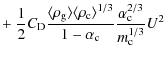
friction. The interclump gas is accelerated in terms of drag between
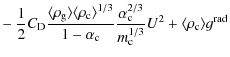
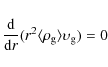
the clump and interclump gas. Thus the mass and momentum equations for
the two-phase flow can be written as
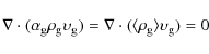
|
(1) |
and
with the constraint

|
(3) |
In these equations,
where
|
(6) |
with
To solve the set of coupled nonlinear differential equations,
we need a powerful numerical method. However, I only
consider the motion of the interclump gas. The velocity structure of
the clump is
assumed to be ![]() law
law
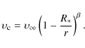
|
(7) |
Thus I only solve Eqs. (1) and (4). In the spherical coordinates, Eqs. (1) and (4) can be written as
|
(8) |
and

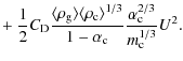
Hydrodynamic equations for the interclumpt gas are described by Eqs. (8) and (9).
2.2 Numerical solution
The solution of the differential Eqs. (8) and (9) can
be obtained by a numerical method. I selected the
Newton-Raphson method to solve the question. The method requests
initialization to both velocity
and density. According to
Eqs. (3), (6), (8), and (9),
we obtain
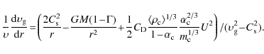
|
(10) |
The equation considered here essentially has the similar structure as the solar wind. The velocity structure is independent of the density. The momentum equation has a singularity at the point where
To account for the influence of wind clumping, the method
described by Abbott (1981) is adopted. The mass-loss rate is defined
from the mean density,

|
(11) |
and
![\begin{displaymath}%
\langle \rho \rangle =\frac{1}{\triangle
V}\int[\alpha_{\rm c}\rho_{\rm c}+(1-\alpha_{\rm c})\rho_{\rm g}]{\rm d}V,
\end{displaymath}](/articles/aa/full_html/2010/04/aa12872-09/img49.png)
|
(12) |
where
To calculate the velocity structure of the interclump gas the
inner boundary densities for both component have to be set.
I assume that the inner velocity of the clump is the sound
velocity. The inner boundary density, ![]() , is
determined by the velocity at the inner boundary and
, is
determined by the velocity at the inner boundary and ![]() .
The density of the gas is assumed to be a factor 10 lower than that of
the clump.
.
The density of the gas is assumed to be a factor 10 lower than that of
the clump.
3 X-ray
The typical O-type stars ![]() Ori A and
Ori A and ![]() Pup
are ideal candidates for testing models about X-ray emission because
they have been studied in detail (Feldmeier et al. 1997b; Waldron
& Cassineli 2000;
Cassineli et al. 2001; Leutenegger et al. 2006b; Pollock 2007; Raassen
et al. 2008).
An important test for this model is to compare the X-ray
temperatures. To estimate the postshock temperature,
I take
Pup
are ideal candidates for testing models about X-ray emission because
they have been studied in detail (Feldmeier et al. 1997b; Waldron
& Cassineli 2000;
Cassineli et al. 2001; Leutenegger et al. 2006b; Pollock 2007; Raassen
et al. 2008).
An important test for this model is to compare the X-ray
temperatures. To estimate the postshock temperature,
I take ![]()
![]()
![]() ,
where U is the relative velocity between
the interclump gas and the clump. In fact, shocks can only
exist in supersonic flows. Thus, in this model I used the
above formula to calculate the post-shock temperatures when the
relative velocity between the clump and the gas is higher than the
sound velocity. The observed temperatures and locations of X-ray
sources are obtained from Waldron & Cassinelli (2007).
(An Erratum
about the paper was published in ApJ, 680, 1595, so I used the
revised data.) The radii
,
where U is the relative velocity between
the interclump gas and the clump. In fact, shocks can only
exist in supersonic flows. Thus, in this model I used the
above formula to calculate the post-shock temperatures when the
relative velocity between the clump and the gas is higher than the
sound velocity. The observed temperatures and locations of X-ray
sources are obtained from Waldron & Cassinelli (2007).
(An Erratum
about the paper was published in ApJ, 680, 1595, so I used the
revised data.) The radii
![]() ,
which were determined by using the He-like ions, denote the local radii
in which the emission lines of different elements are formed. One might
be problematic for the radii whether these thin shells can represent
the range in which each element is formed. In generally, the
spectral lines seem to be formed over a large range. However, the line
emission is proportional to
,
which were determined by using the He-like ions, denote the local radii
in which the emission lines of different elements are formed. One might
be problematic for the radii whether these thin shells can represent
the range in which each element is formed. In generally, the
spectral lines seem to be formed over a large range. However, the line
emission is proportional to ![]() ,
so the observed lines should be dominated by the densest
regions. Thus, it is reasonable to depict a
characteristic radius to each element line. The X-ray
temperatures determined by the H-like-to-He-like line ratios can
represent the average temperatures of the He-like ions and H-like ions
for these element. The temperatures should be somewhat higher than
those of He-like ions. The lack of observed data forced me to use the
average temperatures to denote the temperatures of He-like ions.
In fact, the final results of this model should be corrected
for this discordance. For both stars
,
so the observed lines should be dominated by the densest
regions. Thus, it is reasonable to depict a
characteristic radius to each element line. The X-ray
temperatures determined by the H-like-to-He-like line ratios can
represent the average temperatures of the He-like ions and H-like ions
for these element. The temperatures should be somewhat higher than
those of He-like ions. The lack of observed data forced me to use the
average temperatures to denote the temperatures of He-like ions.
In fact, the final results of this model should be corrected
for this discordance. For both stars ![]() Ori A and
Ori A and ![]() Pup,
the X-ray temperatures for the sulfur are greater than 10 MK.
However, there is no definite observational data in Waldron
& Cassinelli (2007).
Thus, I neglect to fit the temperature for sulfur.
In fact, such high temperature is incompatible with wind
shocks. Schulz et al. (2003)
have revealed similar phenomena in young stars
Pup,
the X-ray temperatures for the sulfur are greater than 10 MK.
However, there is no definite observational data in Waldron
& Cassinelli (2007).
Thus, I neglect to fit the temperature for sulfur.
In fact, such high temperature is incompatible with wind
shocks. Schulz et al. (2003)
have revealed similar phenomena in young stars
![]() Ori A, C,
and E. The hottest X-ray lines appear to originate closest to
the stars since the observed HWHM values are significantly
lower than the wind terminal velocity. (The HWHMs for
Ori A, C,
and E. The hottest X-ray lines appear to originate closest to
the stars since the observed HWHM values are significantly
lower than the wind terminal velocity. (The HWHMs for ![]() Scorpii
are also found to be essentially identical to the HWHMs observed in
late-type stars.) Schulz et al. (2003) show that
these hottest lines are the likely result of magnetic confinement. Some
magnetic confined models have been considered by Babel &
Montmerle (1997), Ud-Doula & Owocki (2002), and Mullan
& Waldron (2006).
Scorpii
are also found to be essentially identical to the HWHMs observed in
late-type stars.) Schulz et al. (2003) show that
these hottest lines are the likely result of magnetic confinement. Some
magnetic confined models have been considered by Babel &
Montmerle (1997), Ud-Doula & Owocki (2002), and Mullan
& Waldron (2006).
Table 1: Line widths of the program stars.
4 Numerical results
Stellar parameters were taken from Table 1 of Feldmeier et al. (1997b). The mass-loss rates are not corrected for the clumping.
For searching the best fits between the observed and
theoretical X-ray locations and temperatures, I used
a ![]() method
to match the observations. To demonstrate the sensitivity of
the motion of
the interclump gas to these parameters, I tested a number of
possible cases. For each individual star, I computed the X-ray
temperatures with the values of
method
to match the observations. To demonstrate the sensitivity of
the motion of
the interclump gas to these parameters, I tested a number of
possible cases. For each individual star, I computed the X-ray
temperatures with the values of ![]() chosen in the range of 0.5-1. The mass of the clump was chosen from a
wide range. Moreover, these models were calculated with the constant
filling factors throughout the winds. For completeness, the observed
MEG, HEG, and their average X-ray temperatures are plotted in
Figs. 1
and 2.
By finding the minimum differences with the average values,
the best-fit parameters were determined for individual objects.
chosen in the range of 0.5-1. The mass of the clump was chosen from a
wide range. Moreover, these models were calculated with the constant
filling factors throughout the winds. For completeness, the observed
MEG, HEG, and their average X-ray temperatures are plotted in
Figs. 1
and 2.
By finding the minimum differences with the average values,
the best-fit parameters were determined for individual objects.
Figure 1
shows that the model with ![]() ,
,
![]() ,
and
,
and ![]() is the best-fit model for O-type supergiant
is the best-fit model for O-type supergiant ![]() Ori A,
but it produces a lower temperature for Silicon. Waldron
& Cassinelli (2000)
find that the Si XIII line originates
in the base of the wind (
Ori A,
but it produces a lower temperature for Silicon. Waldron
& Cassinelli (2000)
find that the Si XIII line originates
in the base of the wind (
![]() )
and suggest that the velocity there is too low to produce the shock
jump. However, Leutenegger et al. (2006a) report a
very different value of 2.1 R*,
which does not agree with the result of Waldron & Cassinelli (2007).
In theirs multi-temperature calculations, Raassen
et al. (2008)
show that the X-ray temperatures were in the range
of 0.85-6.4 Mk. This is in good agreement
with our results. In the
model, the maximum relative velocity between the clump and interclump
gas is about 710
)
and suggest that the velocity there is too low to produce the shock
jump. However, Leutenegger et al. (2006a) report a
very different value of 2.1 R*,
which does not agree with the result of Waldron & Cassinelli (2007).
In theirs multi-temperature calculations, Raassen
et al. (2008)
show that the X-ray temperatures were in the range
of 0.85-6.4 Mk. This is in good agreement
with our results. In the
model, the maximum relative velocity between the clump and interclump
gas is about 710
![]() at R=1.95 R*,
which is high enough to produce the higher temperature at the base of
the wind. The model with m=5
at R=1.95 R*,
which is high enough to produce the higher temperature at the base of
the wind. The model with m=5 ![]()
![]() ,
,
![]() ,
and
,
and ![]() produces higher temperature distributions at the region of
low-temperature regions (see dashed line). Evidently, model
with
produces higher temperature distributions at the region of
low-temperature regions (see dashed line). Evidently, model
with ![]() ,
,
![]() ,
and
,
and ![]() predicted
flatter temperature distributions in the majority of the winds
(see dotted line). If the mass of the clump is
greater than
predicted
flatter temperature distributions in the majority of the winds
(see dotted line). If the mass of the clump is
greater than ![]() ,
the X-ray temperatures predicted by this model will produce a higher
temperature distribution in the whole wind.
,
the X-ray temperatures predicted by this model will produce a higher
temperature distribution in the whole wind.
![\begin{figure}
\par\includegraphics[width=7.5cm,clip]{12872fg1.eps}
\end{figure}](/articles/aa/full_html/2010/04/aa12872-09/img70.png)
|
Figure 1:
The X-ray temperature distributions with different value of the mass,
velocity law, and filling factor of the clump for |
| Open with DEXTER | |
![\begin{figure}
\par\includegraphics[width=7.5cm,clip]{12872fg2.eps}
\end{figure}](/articles/aa/full_html/2010/04/aa12872-09/img71.png)
|
Figure 2:
The X-ray temperature distributions with different
velocity law of the clump for |
| Open with DEXTER | |
For ![]() Pup, the best-fit model is
Pup, the best-fit model is ![]() ,
,
![]() ,
and
,
and ![]() (Fig. 2).
For indicating the influence of velocity structure of the clump on the
X-ray temperature distributions, the models with different values of
(Fig. 2).
For indicating the influence of velocity structure of the clump on the
X-ray temperature distributions, the models with different values of ![]() are also shown in Fig. 2.
These models with higher
are also shown in Fig. 2.
These models with higher ![]() predict the reasonable X-ray temperatures of elements except for
silicon. On the previous analysis for the X-ray luminosity
predict the reasonable X-ray temperatures of elements except for
silicon. On the previous analysis for the X-ray luminosity ![]() ,
Lucy & White (1980)
estimated the mass of the clump is about
,
Lucy & White (1980)
estimated the mass of the clump is about ![]() ,
which is different with the result of this model. However,
as pointed by Lucy & White (1980): ``
,
which is different with the result of this model. However,
as pointed by Lucy & White (1980): ``![]() is
gratifyingly insensitive to m ...''.
Thus, the mass of the clump could not be
constrained well by their model. In this model, the the
highest post-shock temperature is
is
gratifyingly insensitive to m ...''.
Thus, the mass of the clump could not be
constrained well by their model. In this model, the the
highest post-shock temperature is ![]()
![]()
![]() ,
and the corresponding velocity difference is 700
,
and the corresponding velocity difference is 700
![]() at R=1.99 R*
while Lucy & White (1980)
predicted a maximum relative velocity
at R=1.99 R*
while Lucy & White (1980)
predicted a maximum relative velocity ![]() ,
and the corresponding highest temperature is 1.4
,
and the corresponding highest temperature is 1.4 ![]()
![]() at R=1.31 R*.
The result is significantly different from that of this model and is
lower than that of observations.
at R=1.31 R*.
The result is significantly different from that of this model and is
lower than that of observations.
The clump masses cannot be determined by observations. Thus,
I redefine the clump masses by the mass-loss rate. The
mass-flow rate in a clump is
![]() ,
where
,
where ![]() is
the flow time. For our program stars, the flow time can be estimated
by
is
the flow time. For our program stars, the flow time can be estimated
by
![]() ;
therefore, a clump carries about
;
therefore, a clump carries about ![]() for
for ![]() Ori A
and
Ori A
and ![]() for
for ![]() Pup.
Pup.
Leutenegger et al. (2006a) present a
comparison of their measurements to those of Waldron &
Cassinelli (2000)
and Cassinelli et al. (2001).
Table 6 of Leutenegger et al. (2006a) show that
the minimum radius extends to nearly the surface of the star. The shock
jump required for S XV should be higher than that of
Si XIII. This hints that either a steeper velocity structure
or a higher mass for the clump, or both, are needed to fit the emission
of sulfur. A velocity law with ![]() < 0.5
does not seem to be supported by observations. In our
numerical experience, the models with a higher mass of the clump cannot
fit the temperatures for other elements. Thus, the fits of the
S XV emission lines can place a strong constraint on
future modeling efforts.
< 0.5
does not seem to be supported by observations. In our
numerical experience, the models with a higher mass of the clump cannot
fit the temperatures for other elements. Thus, the fits of the
S XV emission lines can place a strong constraint on
future modeling efforts.
5 Discussion
As evident in Figs. 1 and 2, the filling factor, mass, and velocity structure of the clump may significantly affect the X-ray temperature distributions. The post-shock temperature is determined by the relative velocity between the clumps and ambient wind. Equation (5) shows that the drag force between the two components is controlled by the mass, velocity law, and filling factor of the clump, as discussed below.
5.1 Parameters
For clumps with the lower mass, the outward drag force is much greater
than gravity at the base of the wind. Thus, the sound point is very
close to the stellar surface. In fact, the velocity
structure of gas is steeper if the sound point appears near the star.
This suggests that the difference in velocity remains relatively small.
If there is no relative motion between the
interclump gas and the clump, the post-shock gas temperature is zero.
I tested the models with different masses of clumps. The
clumps with lower mass produce lower X-ray temperature
distributions. The model with ![]() produces the X-ray temperature distributions, which are almost zero.
The model with
produces the X-ray temperature distributions, which are almost zero.
The model with ![]() improves the X-ray temperature distributions, but they are
much lower than for observations.
improves the X-ray temperature distributions, but they are
much lower than for observations.
The model with higher ![]() will produce a flatter velocity structure than that with
will produce a flatter velocity structure than that with ![]() .
We find that at the base (1-4 R*)
of the wind, the fast accelerated clumps result in a
greater velocity difference than slow accelerated clumps. For normal
OB stars, the determination of velocity law from
observations is described by
.
We find that at the base (1-4 R*)
of the wind, the fast accelerated clumps result in a
greater velocity difference than slow accelerated clumps. For normal
OB stars, the determination of velocity law from
observations is described by ![]() (Garmany et al. 1981;
Groenewegen & Lamers 1989).
By fitting the far-ultraviolet line P
v, Fullerton et al. (2006) obtained
(Garmany et al. 1981;
Groenewegen & Lamers 1989).
By fitting the far-ultraviolet line P
v, Fullerton et al. (2006) obtained ![]() for
for ![]() Ori A
and 0.5 for
Ori A
and 0.5 for ![]() Pup.
Their results are very close to the value of this model for
Pup.
Their results are very close to the value of this model for ![]() Pup,
but different from that of
Pup,
but different from that of ![]() Ori A.
In fact, if the winds are composed of two components,
the observed value of
Ori A.
In fact, if the winds are composed of two components,
the observed value of ![]() should be greater than 0.5 because it is a weighted average of
the clumps and ambient gas.
should be greater than 0.5 because it is a weighted average of
the clumps and ambient gas.
A small filling factor implies that the mass-loss rates are
decreased a large factor. In this model the filling factor of the
best-fit models for ![]() Ori A
is 0.015 and
Ori A
is 0.015 and ![]() Pup
is 0.01. The X-ray temperatures are very sensitive to the
filling factor of the clump,
Pup
is 0.01. The X-ray temperatures are very sensitive to the
filling factor of the clump,
![]() .
The increase in filling factor by a factor 3 can
result in a lower X-ray temperature distribution.
.
The increase in filling factor by a factor 3 can
result in a lower X-ray temperature distribution.
In this paper, I used a constant filling factor.
In fact, the filing factor may be variable with the radius. In
the quantitative spectral analysis for O stars
HD 190429 and HD 96715 Bouret et al. (2005) use an
exponentially degressive filling factor. However, Puls et al. (2006) have found the
lower clumping factor (the clumping factor is inversely
proportional to the volume filling factor, namely, ![]() )
in the outmost than the inner
wind. Moreover, hydrodynamic simulation (Runacres & Owocki 2002) predict that
the clumping factor is variable with time. Thus, constraining the
filling factor from theoretical model becomes an important
issue.
)
in the outmost than the inner
wind. Moreover, hydrodynamic simulation (Runacres & Owocki 2002) predict that
the clumping factor is variable with time. Thus, constraining the
filling factor from theoretical model becomes an important
issue.
Waldron & Cassinelli (2007) find a
one-to-one correspondence between
![]() and their associated X-ray continuum optical depth unity radii (
and their associated X-ray continuum optical depth unity radii (
![]() )
when the traditional mass-loss rates were adopted, and explained this
as density dependence. For completeness,
I also calculated the dependence of mass-loss rates on X-ray
temperature distributions. The model with a higher mass-loss rate
underestimates the X-ray temperature distributions, reflecting the
consistency between observation and theory, meaning that the mass loss
rate should be decreased.
)
when the traditional mass-loss rates were adopted, and explained this
as density dependence. For completeness,
I also calculated the dependence of mass-loss rates on X-ray
temperature distributions. The model with a higher mass-loss rate
underestimates the X-ray temperature distributions, reflecting the
consistency between observation and theory, meaning that the mass loss
rate should be decreased.
5.2 X-ray emission lines
I also compared the widths of the X-ray emission lines. In
Table 1,
I list the line widths for O VII, Ne IX,
Mg XI, and Si XIII. I used a half of the
local velocity to represent the theoretical value. The fact that the
theoretical line widths increase outward through the
wind indicates that the lines occur in the accelerated region of the
wind. I also notice that the observed widths are very
different for the different authors. Cohen et al. (2006) determine the
value of the line widths of ![]() Ori, which are
500+120-70 and
1360+160-150
Ori, which are
500+120-70 and
1360+160-150
![]() for O VII and Ne Ix; however, the values measured by
Waldron & Cassinelli (2000)
are 900
for O VII and Ne Ix; however, the values measured by
Waldron & Cassinelli (2000)
are 900 ![]()
![]() .
The theoretical results agree with the values of Waldron &
Cassinelli (2000).
It is not clear why the theoretical results contradict the
observations of Cohen et al. (2006).
In fact, the emission line analysis of
.
The theoretical results agree with the values of Waldron &
Cassinelli (2000).
It is not clear why the theoretical results contradict the
observations of Cohen et al. (2006).
In fact, the emission line analysis of ![]() Ori from Cohen
et al. shows that there is significant blueshift, but Waldron
& Cassinelli find that the lines are almost symmetric, and the
velocity dispersions for all X-ray line are in the range 900
Ori from Cohen
et al. shows that there is significant blueshift, but Waldron
& Cassinelli find that the lines are almost symmetric, and the
velocity dispersions for all X-ray line are in the range 900 ![]()
![]() .
Thus, another observation may be needed to distinguish the
contradiction.
.
Thus, another observation may be needed to distinguish the
contradiction.
For the spectrum of ![]() Pup, there are no corresponding values for
ions O VII, Ne IX, Mg XI, and
Si XIII from the published literature. In the XMM
spectrum of
Pup, there are no corresponding values for
ions O VII, Ne IX, Mg XI, and
Si XIII from the published literature. In the XMM
spectrum of ![]() Pup
(Kahn et al. 2001),
the high Z lines have characteristic widths
Pup
(Kahn et al. 2001),
the high Z lines have characteristic widths
![]() .
In their Table 2 Cassinelli et al. (2001) list the line
widths of some ions, with the HWHM of
.
In their Table 2 Cassinelli et al. (2001) list the line
widths of some ions, with the HWHM of ![]() .
These values are comparable to the theoretical results.
.
These values are comparable to the theoretical results.
6 Conclusion
The spatial X-ray temperature distributions show that the temperature
decreases with the increase in radius of supergiants. The model
predicted the trend and fitted the observed X-ray temperatures.
In fact, the theoretic X-ray temperatures are determined by
the mass, filling factor, and velocity structure of the clump. The
model shows that the range in mass of clump is about ![]() ;
otherwise, the model cannot predict significant X-ray temperatures. The
results are also sensitive to the velocity law. The models with the
exponent of the clump velocity
;
otherwise, the model cannot predict significant X-ray temperatures. The
results are also sensitive to the velocity law. The models with the
exponent of the clump velocity ![]() can produce a large shock jump near the stellar surface and fit the
observations. For the whole wind, a flatter velocity structure is
possible because of the counteraction of velocity structure of the
clump and interclump gas. Compared with the smooth-wind models, this
model also shows that the winds of O-type suergiants are strongly
clumped and the mass loss rates could
decrease by a factor of 8-10. The model also predicts the line widths
of O VII, Ne IX, Mg XI, and
Si XIII for the
can produce a large shock jump near the stellar surface and fit the
observations. For the whole wind, a flatter velocity structure is
possible because of the counteraction of velocity structure of the
clump and interclump gas. Compared with the smooth-wind models, this
model also shows that the winds of O-type suergiants are strongly
clumped and the mass loss rates could
decrease by a factor of 8-10. The model also predicts the line widths
of O VII, Ne IX, Mg XI, and
Si XIII for the ![]() Pup
and the
Pup
and the ![]() Ori A.
The theoretical results are consistent with the
values of observations.
Ori A.
The theoretical results are consistent with the
values of observations.
I am grateful to the referee for a constructive suggestion that lead to substantive improvements in this work. This work was supported by the National Natural Science Foundation of China (Nos. 10803018); the Knowledge Innovation Program of Chinese Academy of Sciences (07ACX21001), and Western Light Talent Culture Project of The Chinese Academy of Sciences (08AXB31001).
References
- Abbott, D. C., Bieging, J. H., & Churchwell, E. 1981, ApJ, 250, 645 [NASA ADS] [CrossRef] [Google Scholar]
- Babel, J. 1997, A&A, 323, 121 [NASA ADS] [Google Scholar]
- Bouret, J. C., Lanz, T., Hillier, D. J., et al. 2003, ApJ, 595, 1182 [NASA ADS] [CrossRef] [Google Scholar]
- Bouret, J. C., Lanz, T., & Hillier, D. J. 2005, A&A, 438, 301 [NASA ADS] [CrossRef] [EDP Sciences] [Google Scholar]
- Cassinelli, J. P., & Olson, G. L. 1979, ApJ, 229, 304 [NASA ADS] [CrossRef] [Google Scholar]
- Cassinelli, J. P., Miller, N. A., Waldron, W. L., et al. 2001, ApJ, 554, L55 [NASA ADS] [CrossRef] [Google Scholar]
- Cassinelli, J. P., Ignace, R., Waldron, W. L., et al. 2008, ApJ, 683, 1052 [NASA ADS] [CrossRef] [Google Scholar]
- Cohen, D. H., de Messières, G. E., MacFarlane, J. J., et al. 2003, ApJ, 586, 495 [NASA ADS] [CrossRef] [Google Scholar]
- Cohen, D. H., Leutenegger, M. A., Grizzard, K. T., et al. 2006, MNRAS, 368, 1905 [NASA ADS] [CrossRef] [Google Scholar]
- Feldmeier, A., Puls, J., & Pauldrach, W. A. 1997a, A&A, 322, 878 [NASA ADS] [Google Scholar]
- Feldmeier, A., Kudritzki, R. P., Palsa, R., et al. 1997b, A&A, 320, 899 [NASA ADS] [Google Scholar]
- Fullerton, A. W., Massa, D. L., & Prinja, R. K. 2006, ApJ, 637, 1025 [NASA ADS] [CrossRef] [Google Scholar]
- Garmany, C. D., Olson, G. L., & van Steenberg, M. E. 1981, ApJ, 250, 660 [NASA ADS] [CrossRef] [Google Scholar]
- Groenewegen, M. A. T., & Lamers, H. J. G. L. M. 1989, A&AS, 79, 359 [NASA ADS] [Google Scholar]
- Guo, J. H. 2008, IAUS, 252, 341 [NASA ADS] [CrossRef] [Google Scholar]
- Howk, J. C., Cassinelli, J. P., Bjorkman, J. E., & Lamers, H. J. G. L. M. 2000, ApJ, 534, 348 [NASA ADS] [CrossRef] [Google Scholar]
- Kahn, S. M., Leutenegger, M. A., Cottam, J., et al. 2001, A&A, 365, L312 [NASA ADS] [CrossRef] [EDP Sciences] [Google Scholar]
- Kramer, R., Cohen, D. H., & Owocki, S. P. 2006, ApJ, 592, 532 [Google Scholar]
- Leutenegger, M. A., Paerels, F. B. S., Kahn, S. M., & Cohen, D. H. 2006a, ApJ, 650, 1096 [NASA ADS] [CrossRef] [Google Scholar]
- Leutenegger, M. A., Owocki, S. P., Kahn, S. M., & Paerels, B. S. 2006b, ApJ, 659, 642 [Google Scholar]
- Lucy, L. B. 1982, ApJ, 255, 284 [Google Scholar]
- Lucy, L. B., & Solomon, P. M. 1970, ApJ, 159, 879 [NASA ADS] [CrossRef] [Google Scholar]
- Lucy, L. B., & White, R. L. 1980, ApJ, 241, 300 [NASA ADS] [CrossRef] [Google Scholar]
- Mullan, D. J., & Waldron, W. L. 2006, ApJ, 637, 506 [NASA ADS] [CrossRef] [Google Scholar]
- Owocki, S. P., & Cohen, D. H. 2006, ApJ, 648, 565 [NASA ADS] [CrossRef] [Google Scholar]
- Owocki, S. P., & Puls, J. 1999, ApJ, 510, 355 [NASA ADS] [CrossRef] [Google Scholar]
- Owocki, S. P., Castor, J. I., & Rybicki, G. B. 1988, ApJ, 335, 914 [NASA ADS] [CrossRef] [Google Scholar]
- Pollock, A. M. T. 2007, A&A, 463, 1111 [NASA ADS] [CrossRef] [EDP Sciences] [Google Scholar]
- Pistinner, S., & Shaviv, G. 1993, ApJ, 414, 612 [NASA ADS] [CrossRef] [Google Scholar]
- Puls, J., Markova, N., Scuderi, S., et al. 2006, A&A, 454, 625 [NASA ADS] [CrossRef] [EDP Sciences] [Google Scholar]
- Raassen, A. J. J., van der Hucht, K. A., Millier, N. A., & Cassinelli, J. P. 2008, A&A, 478, 513 [NASA ADS] [CrossRef] [EDP Sciences] [Google Scholar]
- Runacres, M. C., & Owocki, S. P. 2002, A&A, 381, 1015 [NASA ADS] [CrossRef] [EDP Sciences] [Google Scholar]
- Schulz, N. S., Canizares, C., Huenemoerder, D., & Tibbets, K. 2003, ApJ, 595, 365 [NASA ADS] [CrossRef] [Google Scholar]
- ud-Doula, A., & Owocki, S. P. 2002, ApJ, 576, 413 [NASA ADS] [CrossRef] [Google Scholar]
- Waldron, W. L. 2005, in ITAMP Workshop: X-ray Diagnostics of Astrophysical plasma (New York: AIP), AIP Conf. Ser., 774, 353 [Google Scholar]
- Waldron, W. L., & Cassinelli, J. P. 2000, ApJ, 548, L45 [Google Scholar]
- Waldron, W. L., & Cassinelli, J. P. 2007, ApJ, 668, 456 [NASA ADS] [CrossRef] [Google Scholar]
All Tables
Table 1: Line widths of the program stars.
All Figures
|
|
Figure 1:
The X-ray temperature distributions with different value of the mass,
velocity law, and filling factor of the clump for |
| Open with DEXTER | |
| In the text | |
|
|
Figure 2:
The X-ray temperature distributions with different
velocity law of the clump for |
| Open with DEXTER | |
| In the text | |
Copyright ESO 2010
Current usage metrics show cumulative count of Article Views (full-text article views including HTML views, PDF and ePub downloads, according to the available data) and Abstracts Views on Vision4Press platform.
Data correspond to usage on the plateform after 2015. The current usage metrics is available 48-96 hours after online publication and is updated daily on week days.
Initial download of the metrics may take a while.