Fitting formulae of the reduced-shear power spectrum for weak lensing

M. Kilbinger

doi:10.1051/0004-6361/201014829

Home

All issues

Volume 519 (September 2010)

A&A, 519 (2010) A19

Full HTML

Free Access

Issue		A&A Volume 519, September 2010


Article Number		A19
Number of page(s)		7
Section		Cosmology (including clusters of galaxies)
DOI		https://doi.org/10.1051/0004-6361/201014829
Published online		07 September 2010

A&A 519, A19 (2010)

Fitting formulae of the reduced-shear power spectrum for weak lensing (Research Note)

M. Kilbinger^1,2,3

1 - Excellence Cluster Universe, Technische Universität München, Boltzmannstr. 2, 85748 Garching, Germany
2 - Universitäts-Sternwarte München, Scheinerstr. 1, 81679 München, Germany
3 - Shanghai Key Lab for Astrophysics, Shanghai Normal University, Shanghai 200234, PR China

Received 20 April 2010 / Accepted 9 June 2010

Abstract
Context. Weak gravitational lensing is a powerful probe of large-scale structure and cosmology. Most commonly, second-order correlations of observed galaxy ellipticities are expressed as a projection of the matter power spectrum, corresponding to the lowest-order approximation between the projected and the three-dimensional power spectrum.
Aims. The dominant lensing-only contribution beyond the zero-order approximation is the reduced shear, which takes into account not only lensing-induced distortions but also the isotropic magnification of galaxy images. This involves an integral over the matter bispectrum. We provide a fast and general way to calculate this correction term.
Methods. Using a model for the matter bispectrum, we fit elementary functions to the reduced-shear contribution and its derivatives with respect to cosmological parameters. The dependence on cosmology is encompassed in a Taylor-expansion around a fiducial model.
Results. Within a region in parameter space comprising the WMAP7 68% error ellipsoid, the total reduced-shear power spectrum (shear plus fitted reduced-shear correction) is accurate to 1% (2%) for $\ell <10^4$ ( $\ell <2 \times 10^5$ ). This corresponds to a factor of four reduction in the bias compared to the case where no correction is used. This precision is necessary to match the accuracy of current non-linear power spectrum predictions from numerical simulations.

Key words: gravitational lensing: weak - large-scale structure of Universe

1 Introduction

Cosmic shear surveys exploit the distortions of distant galaxy images induced by the matter structures in the Universe on large scales. Weak cosmological lensing has become an important tool to measure cosmological parameters. The current precision in the measured shapes of high-redshift galaxies is at the few percent level providing important constraints on the matter density $\Omega_{\rm m}$ and the power-spectrum normalisation $\sigma_8$ . Future surveys aim to achieve sub-percent level accuracy in measuring dark-energy properties or deviations from general relativity.

To reach this precision for cosmological parameters, efforts not only on the observational but also on the theoretical side have to be made. To predict the shear power spectrum from theoretical models, several approximations are usually made to facilitate calculations. When comparing and fitting models to observations, these simplifications can significantly bias the resulting cosmological parameters. One of these approximations is to neglect the correction due to the so-called reduced shear.

The observed ellipticity of galaxies is an estimator of the reduced shear

$\begin{displaymath}g = \frac{\gamma}{1 - \kappa}, \end{displaymath}$

(1)

where $\gamma$ is the shear and $\kappa$ is the convergence. Here and in the following, both shear and reduced shear are represented as complex quantities, $\gamma = \gamma_1 + {\rm i}\gamma_2$ , $g = g_1 + {\rm i} g_2$ . Since in weak lensing the convergence is small, $\vert\kappa\vert \ll 1$ , one usually simplifies the above relation to linear order, $g \approx \gamma$ .

The effect of reduced shear was examined using N-body simulations by White (2005) and compared with theoretical predictions in Dodelson et al. (2006). Corrections to the lensing skewness were discussed in Schneider et al. (1998) and Dodelson & Zhang (2005). An extensive study of higher-order corrections to the weak-lensing power spectrum, including reduced shear, was presented by Krause & Hirata (2009). Compared with corrections due to light-path integration (relaxation of the Born approximation) and lens-lens coupling (e.g., Bernardeau et al. 1997; Seitz 1993), reduced-shear corrections represent the dominant contribution to the weak-lensing power spectrum. The lowest-order correction term, which is of order ${\cal O}(\phi^3)$ in the gravitational potential $\phi$ , reaches 10% of the total lensing spectrum. This is the term that we consider in this work. The next-order correction at ${\cal O}(\phi^4)$ is one magnitude below the ${\cal O}(\phi^3)$ -term (Krause & Hirata 2009). Ignoring reduced shear will cause a bias in cosmological parameters, which is comparable to the statistical error from future surveys like DES, LSST, or Euclid (Shapiro 2009). For the weak-lensing results of the COSMOS survey, an estimate from numerical simulations yielded a 1% underestimation of $\sigma_8$ (Schrabback et al. 2010).

Another correction to weak lensing from a magnitude-limited galaxy sample is the so-called magnification bias. Hamana (2001) found its contribution to the lensing power spectrum to be small. The corresponding third-order correction terms were also calculated and compared to numerical simulations by Ménard et al. (2003). However, if not corrected for, future surveys will yield significantly biased cosmological parameter constraints (Schmidt et al. 2009a). The lowest-order correction term has the same functional form as the reduced-shear one, and therefore both can be dealt with simultaneously. Higher-order terms contribute by smaller than one percent to the lensing power spectrum (Krause & Hirata 2009).

There are additional important sources of contamination to the weak lensing observables, some of which may be larger than the reduced-shear corrections. These involve galaxy clustering, the intrinsic alignment of galaxies with each other or with the surrounding dark matter haloes, and the modelling of the non-linear dark-matter power spectrum and baryonic processes. The modelling of these effects requires detailed understanding of baryonic physics, galaxy formation, the interplay between galaxies and dark matter, and massive numerical simulations in the case of the non-linear power spectrum. In contrast, taking into account the reduced shear is straightforward and can be done with sufficient accuracy to render it a sub-dominant contamination.

In the next section, we review the expressions for the lowest-order reduced-shear term, and introduce a fitting scheme to efficiently model this term. In Sect. 3, we present our results, demonstrating the accuracy of the fits. We conclude this paper in Sect. 4.

2 Reduced shear

2.1 Lowest-order expansion

For small values of the convergence, $\vert\kappa\vert < 1$ , the reduced shear (1) is expanded as

$\begin{displaymath}g = \frac{\gamma}{1-\kappa} = \gamma [ 1 + \kappa + \kappa^2 + \ldots ]. \end{displaymath}$

(2)

To calculate the power spectrum of the reduced shear g, we apply a Fourier transform to Eq. (2) to second order

$\begin{displaymath}\hat g(\vec \ell) \approx \hat \gamma(\vec \ell) + (\hat \gamma * \hat \kappa)(\vec \ell). \end{displaymath}$

(3)

In our notation, the convolution of $\hat \gamma$ and $\hat \kappa$ is

$\begin{displaymath}(\hat \gamma * \hat \kappa)(\vec \ell) = \int \frac{{\rm d}^... ...(\vec \ell^\prime) \hat \kappa(\vec \ell - \vec \ell^\prime). \end{displaymath}$

(4)

We assume that the reduced shear is measured in redshift bins. With P_g^mn, we denote the reduced-shear (cross-)power spectrum for two redshift bins with indices m and n. In general, the shear field can be decomposed into an E-mode (gradient) and a B-mode (curl). However, as is the case for cosmic shear at lowest order, the reduced-shear correction of order ${\cal O}(\phi^3)$ does not have a B-mode component (Schneider et al. 2002), and in the following we focus only on the E-mode. In the absence of a B-mode, the reduced-shear power spectrum is defined to be (Schneider et al. 2002)

$\begin{displaymath}\left\langle \hat g^m(\vec \ell) {\hat g^n}{^*}(\vec \ell^\pr... ...\delta_{\rm D}(\vec \ell - \vec \ell^\prime) P^{mn}_{g}(\ell), \end{displaymath}$

(5)

where g^m denotes the reduced shear measured from galaxies in the mth redshift bin, the asterisk (^*) denotes complex conjugation, and $\delta_{\rm D}$ is the Dirac delta-function.

The reduced-shear power spectrum is the sum of the convergence power spectrum (which equals the shear power spectrum) and a correction given by

		$\displaystyle P^{mn}_{g}(\ell) \approx P^{mn}_{\kappa}(\ell) + {P^{(1)}}^{mn}_{g}(\ell);$	(6)
		$\displaystyle (2\pi)^2 \delta_{\rm D}(\vec \ell - \vec \ell^\prime) {P^{(1)}}^{... ...at \kappa^n \right)}^*(\vec \ell^\prime) \right\rangle + (m \leftrightarrow n).$	(7)

Using the relation between shear and convergence, $\hat \gamma(\vec \ell) = \exp(2{\rm i}\beta) \hat \kappa(\vec \ell)$ , where $\beta$ is the polar angle of the wave vector $\vec \ell$ , and that the convergence is a real field, $\hat \kappa^*(\vec \ell) = \hat \kappa(-\vec \ell)$ , the third-order correlator in Eq. (7) can be written in terms of the convergence bispectrum $B_\kappa$ , which is defined by the equation

$\begin{displaymath}\left\langle \hat \kappa^m(\vec \ell_1) \hat \kappa^n(\vec \e... ...ll_2 + \vec \ell_3) B^{mnp}_\kappa(\vec \ell_1, \vec \ell_2). \end{displaymath}$

(8)

With this, we derive the correction term

$\begin{displaymath}{P^{(1)}}^{mn}_{g}(\ell) = \int \frac{{\rm d}^2\ell^{\prime}... ...) + B^{nmm}_\kappa(\vec \ell_0, -\vec \ell^{\prime}) \right]. \end{displaymath}$

(9)

Without loss of generality, we have set $\beta = 0$ and introduced $\vec \ell_0 = (\ell, 0)$ . In the integrand, $\beta^\prime$ is the polar angle of $\vec \ell^\prime$ .

The convergence bispectrum can be expressed in terms of the three-dimensional matter bispectrum $B_\delta$ using Limber's equation (Limber 1953; Kaiser 1992) providing

		$\displaystyle B_\kappa^{mnp}(\vec \ell_1, \vec \ell_2) = \int_{a_{\rm lim}}^1 {... ...{\vec \ell_1}{f_K[\chi(a)]}, \frac{\vec \ell_2}{f_K[\chi(a)]}; \chi(a) \right);$
		$\displaystyle F^{mnp}(a) = \frac{{\rm d}\chi}{{\rm d}a} \frac{G^m(a)G^n(a)G^p(a)}{f_K[\chi(a)]}\cdot$	(10)

The lower limit of the integral over the scale factor a corresponds to the limiting redshift, $a_{\rm lim} = 1/(1+z_{\rm lim})$ , $\chi$ is the comoving distance, and f_K is the comoving angular diameter distance. The lensing efficiency G^m for the mth redshift bin is

$\begin{displaymath}G^m(a) = \frac 3 2 \left(\frac{H_0}c\right)^2 \frac{\Omega_{\... ...me) \frac{f_K[\chi(a^\prime) - \chi(a)]}{f_K[\chi(a^\prime)]}, \end{displaymath}$

(11)

which includes an integral over the probability distribution p_m of the number density of source galaxies in the mth bin.

2.2 Expansion around a fiducial model

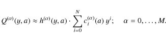
In the expressions needed to calculate the first-order reduced-shear power spectrum in Eqs. (9, 10), we can interchange the $\ell$ - and the a-integration, and replace the latter by a finite sum. Then

		$\displaystyle {P^{(1)}}^{mn}_{g}(\ell) \approx \Delta a \sum_{k=1}^{N_a} \bar F^{mn}(a_k) Q(\ell, a_k);$
		$\displaystyle \bar F^{mn}(a) = \frac 1 2 \left[ F^{mnn}(a_k) + F^{nmm}(a_k) \right];$
		$\displaystyle Q(\ell, a) = 2 \int \frac{{\rm d}^2 \ell^\prime}{(2\pi)^2} \cos (... ...ac{\vec\ell_0}{f_K[\chi(a)]}, \frac{-\vec\ell^\prime}{f_K[\chi(a)]}\right)\cdot$	(12)

Evaluating the $\ell^\prime$ -integral is not a difficult but very time-consuming numerical problem. It is significantly slower than the calculation of the matter power spectrum necessary for the convergence power spectrum. This makes reduced-shear corrections the limiting factor in the parameter analysis of a weak-lensing survey, for example using Monte Carlo sampling. In the following, we present fitting formulae that provide an accurate approximation for this term within a region in parameter space around a fiducial cosmological model. The $\ell$ -independent term F^mnn(a) is easily computed and can be tabulated. Since it depends on the source redshift distribution, it has to be determined for each survey.

Table 1: Parameter limits for where the accuracy of the fitted reduced-shear power spectrum is better than $1\%$ for $\ell <10^4$ , and better than $2\%$ for $\ell <2 \times 10^5$ (see also Fig. 3).

We perform a Taylor-expansion to first order P^(1)mn_g as a function of a cosmological parameter vector $\vec p = (p_1, p_2, \ldots, p_M)$ around a fiducial cosmological model with parameter $\vec p_0$

$\begin{displaymath}{P^{(1)}}^{mn}_{g} (\ell, \vec p) \approx {P^{(1)}}^{mn}_{g} ... ...)}}^{mn}_{g} (\ell, \vec p)\right\vert _{\vec p = \vec p_0}. \end{displaymath}$

(13)

Inserting Eq. (12), the derivatives with respect to cosmological parameters are given by

$\displaystyle \frac{\partial {P^{(1)}}^{mn}_{g}(\ell, \vec p)}{\partial p_\alpha}$	=	$\displaystyle \Delta a \sum_{k=1}^{N_a} \Bigg\{ \bar F^{mn}(a_k, \vec p) \frac{\partial Q(\ell, a_k, \vec p)}{\partial p_\alpha}$
		$\displaystyle +~ \frac{\partial \bar F^{mn}(a_k, \vec p)}{\partial p_\alpha} Q(\ell, a_k, \vec p) \Bigg\}.$	(14)

In Sect. 3, we consider the cosmological parameters $\vec p = (\Omega_{\rm m}, \Omega_{\rm de}, w, \Omega_{\rm b}, h, \sigma_8, n_{\rm s})$ (see also Table 1).

2.3 Magnification and size bias

A typical galaxy sample used in weak cosmological lensing is selected by both magnitude and galaxy size. Magnification due to lensing changes both quantities (e.g. Bartelmann & Schneider 2001), and therefore introduces a correlation between number density and convergence. If the number density of galaxies with fluxes higher than some flux S, and sizes larger than some size R can be written as power laws,

$\begin{displaymath}p({>}S, {>}R) \propto S^{-\alpha} R^{-\beta}, \end{displaymath}$

(15)

the observed number density differs from the unlensed one p₀to first order, becoming

$\begin{displaymath}p = p_0 \left( 1 + q \kappa \right); \qquad q = 2 \left( \alpha + \beta - 1 \right), \end{displaymath}$

(16)

according to Schmidt et al. (2009b,a). This simple linear model assumes that the galaxy selection function depends on flux and size in a separable way. We refer to Wyithe et al. (2003) for a generalisation that takes into account correlations between the two quantities.

Magnification and size bias induces a lowest-order correction to the lensing power spectrum which has the same form as for reduced shear. Therefore, we can add the corresponding correction term ${P^{(1)}}^{mn}_{\mu}$ to Eq. (6) with

		$\displaystyle {P^{(1)}}^{mn}_\mu(\ell) \approx \Delta a \sum_{k=1}^{N_a} \bar F^{mn}(a_k) Q_\mu(\ell, a_k);$
		$\displaystyle Q_\mu(\ell, a) = q Q(\ell, a),$	(17)

where the function Q is given in Eq. (12).

$\begin{figure} \par\includegraphics[width=8cm,clip]{14829Fg1} \end{figure}$	Figure 1: The function $Q^{(0)}(\ell ) = Q(\ell )$ for different scale factors a as indicated in the panel (points), and the composite fitting function (Eq. (21), lines).
Open with DEXTER

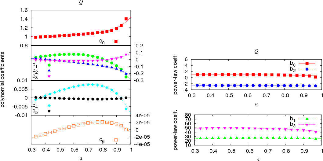
$\begin{figure} \par\resizebox{18cm}{!}{\includegraphics{14829Fg2}} \end{figure}$	Figure 2: Fit coefficients as a function of scale factor. Left: the polynomial fit coefficients c⁽⁰⁾_i for $i=0, \ldots, N=6$ (Eq. (21)). The lines are polynomials in a or order N_c = 3. Right: the power-law coefficients $b^{(0)}_i, i=0, \ldots, 3$ of the composite function h⁽⁰⁾ (Eq. (18)). The lines are polynomials in a of order N_b = 3.
Open with DEXTER

$\begin{figure} \par\resizebox{18cm}{!}{\includegraphics{14829Fg3}}\vspace*{0.5mm} \vspace*{4.25mm} \end{figure}$

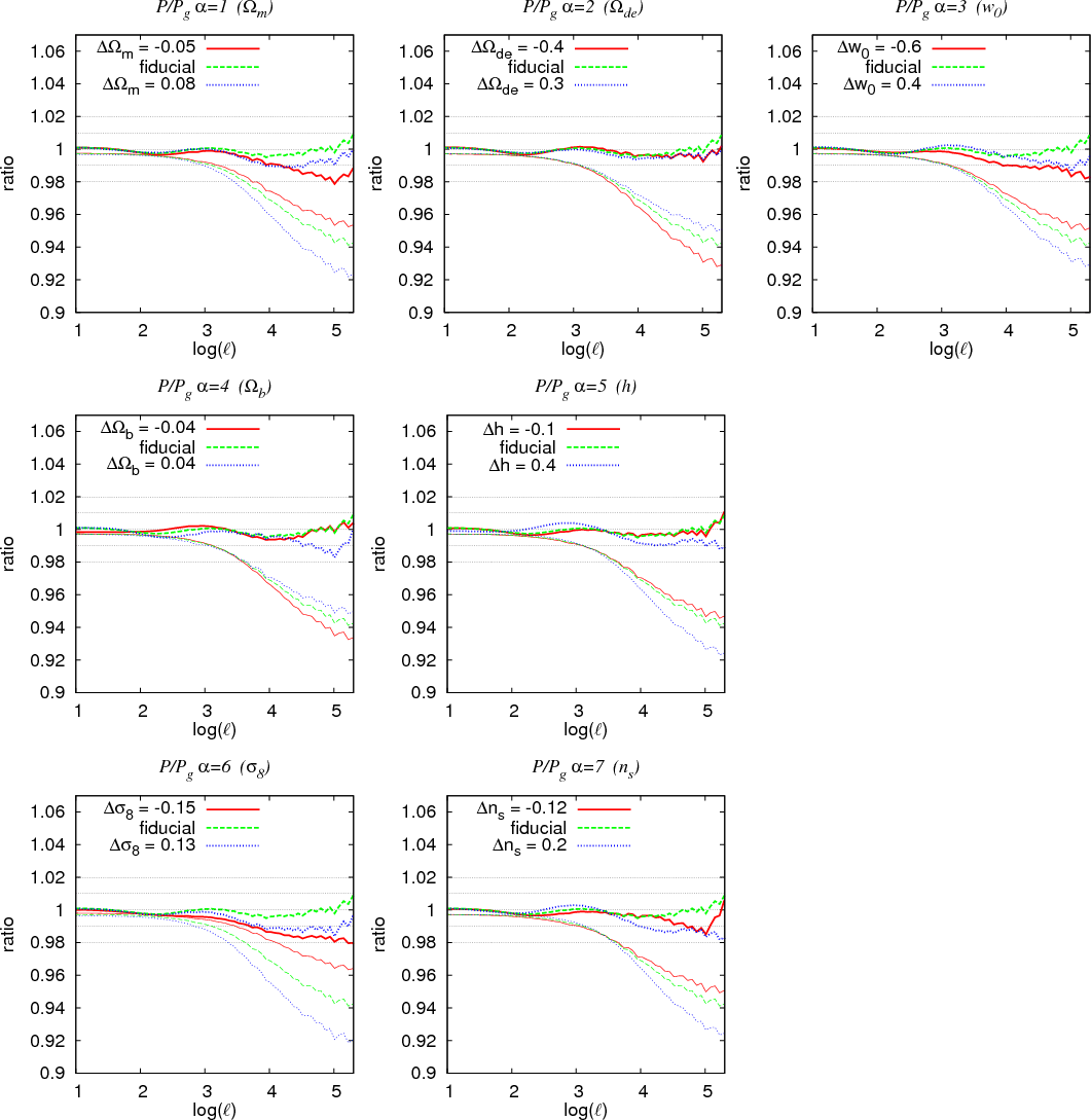
Figure 3:

The fitted reduced-shear power spectrum (thick lines) and the uncorrected convergence power spectrum (thin lines). Both quantities are plotted as ratios with respect to the reduced-shear power spectrum (6), where the first-order correction $P^{(1)}_{\rm g}$ has been obtained by numerical integration of Eq. (12). In each panel, we show the power spectra at the fiducial model (dashed lines) and the lower (solid) and upper (dashed) boundaries within which a 2% accuracy is reached for $\ell <2 \times 10^5$ , see Table 1.

Open with DEXTER

2.4 Fitting formulae

For simplicity, we define Q⁽⁰⁾ = Q and $Q^{(\alpha)} = \partial Q/\partial p_\alpha$ for $\alpha = 1, \ldots, M$ . These correspond to the $\ell$ -dependent terms in Eqs. (12) and (14), which behave as near-power laws for both small and large $\ell$ . With the abbreviation $y=\ln \ell$ , we perform two linear fits of $\ln\left\vert Q^{(\alpha)}(y)\right\vert$ for $y<y_{\rm low} = 3$ and $y>y_{\rm up}=11.5$ , respectively. We smoothly piece together these two asymptotic functions with a cubic spline $s^{\alpha}(y)$ such that the composite function $\ln h^{(\alpha)}(y), \alpha = 0, \ldots, M,$ and its first derivative are continuous

$\displaystyle \ln h^{(\alpha)}(y, a)$

=

$\displaystyle \left\{ \begin{array}{ll} g_{\rm low}^{(\alpha)}(y, a) \quad & \m... ...(\alpha)}(y, a) \quad & \mbox{for} \quad y > y_{\rm up}; \\ \end{array}\right.$

(18)

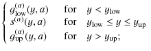
for the linear functions

		$\displaystyle g_{\rm low}^{(\alpha)}(y, a) = b^{(\alpha)}_0(a) \cdot y + b^{(\alpha)}_1(a);$
		$\displaystyle g_{\rm up}^{(\alpha)}(y, a) = b^{(\alpha)}_2(a) \cdot y+ b^{(\alpha)}_3(a),$	(19)

and the cubic spline

		$\displaystyle s^{(\alpha)}(y, a) = \sum_{\nu=0}^{3} r^{(\alpha)}_\nu(a) \cdot \left(\frac{y - y_{\rm low}}{\Delta}\right)^\nu ;$
		$\displaystyle \Delta = y_{\rm up} - y_{\rm low};$
		$\displaystyle r^{(\alpha)}_0(a) = g^{(\alpha)}_{\rm low}(y_{\rm low}, a);$
		$\displaystyle r^{(\alpha)}_1(a) = \Delta \cdot b^{(\alpha)}_0(a);$
		$\displaystyle r^{(\alpha)}_2(a) = 3 g^{(\alpha)}_{\rm up}(y_{\rm up}, a) - \Delta \cdot b^{(\alpha)}_2(a) - 3 r^{(\alpha)}_0(a) - 2 r^{(\alpha)}_1(a) ;$
		$\displaystyle r^{(\alpha)}_3(a) = \Delta \cdot b^{(\alpha)}_2(a) - 2 g^{(\alpha)}_{\rm up}(y_{\rm up}, a) + 2 r^{(\alpha)}_0(a) + r^{(\alpha)}_1(a).$	(20)

The ratios $Q^{(\alpha)} / h^{(\alpha)}$ are then fitted by polynomials of order N in $y=\ln \ell$ , at the fiducial cosmology $\vec p = \vec p_0$ , and for each scale factor $a = a_k, k=1, \ldots, N_a$ ,

$\begin{displaymath}Q^{(\alpha)}(y,a) \approx h^{(\alpha)}(y, a) \cdot \sum_{i=0}^{N} c^{(\alpha)}_i(a) ~ y^i; \;\;\;\; \alpha = 0, \ldots, M. \end{displaymath}$

(21)

We note that we cannot fit the logarithm of the functions $Q^{(\alpha)}$ , since the derivatives of Q with respect to some cosmological parameters change sign.

The fit coefficients $b^{(\alpha)}_i, c^{(\alpha)}_i$ are expected to smoothly vary with the scale factor a. We therefore perform another series of fits by polynomials of order N_b and N_c, respectively

$\begin{displaymath}b^{(\alpha)}_i(a) \approx \sum_{j=0}^{N_b} B^{(\alpha)}_{ij} ... ...alpha)}_i(a) \approx \sum_{j=0}^{N_c} C^{(\alpha)}_{ij} ~ a^j. \end{displaymath}$

(22)

The two matrices $B^{(\alpha)}$ and $C^{(\alpha)}$ for $\alpha = 0, \ldots, M$ defined in the last equation completely determine our approximation for the $\ell$ -dependent terms of the reduced-shear power spectrum correction.

3 Results

We use a fiducial flat $\Lambda$ CDM cosmological model with WMAP7-like parameters, $\Omega_{\rm m}= 0.27, \Omega_{\rm b } = 0.045, h = 0.71, \sigma_8 = 0.8$ and $n_{\rm s} = 0.96$ (Komatsu et al. 2010). The dark-matter bispectrum is calculated according to Scoccimarro & Couchman (2001). Their fitting formula is accurate to only 30-50% on small scales; this is however sufficient for our purpose. We note also that the bispectrum is not calibrated for any dark-energy model other than $\Lambda$ CDM. For the matter power spectrum, we use the ``halofit'' fitting formula of Smith et al. (2003) and the transfer function ``shape fit'' from Eisenstein & Hu (1998). Following the icosmo.org code (Refregier et al. 2008) for models with $w \ne -1$ , we modify ``halofit'' to interpolate between $\Lambda$ CDM and w=-1/3, which behaves in a similar way to an OCDM model (for more details, see Schrabback et al. 2010).

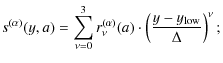
The function Q and the corresponding fit with the composite function given in Eq. (21) are shown in Fig. 1. The polynomial that is part of the composite function has order N=6. The fitting coefficients b⁽⁰⁾_i and c_i⁽⁰⁾ are plotted in Fig. 2. Although the higher-order polynomial coefficients have relatively low amplitudes (right panel), we found that a polynomial of order 6 is necessary to provide a good fit to the reduced-shear power spectrum, as discussed below. For the polynomial fits of the coefficients as functions of a (22), we chose N_b = N_c = 3. These cubic polynomials provide sufficient accuracy, in particular for $a \rightarrow 1$ , where the coefficients show the most variation. This is important because the reduced-shear correction spectrum in Eq. (12) obtains a large contribution from large a.

We perform the fits in the $\ell$ -range between 0.1 and $2 \times 10^5$ . The functions $Q^{(\alpha)}$ are not perfect power laws, therefore the fit for large $\ell$ is not excellent. We found an improvement of our final results for the total power spectrum by adding 0.05 to b₂ after performing the fits.

The fitting functions for the reduced-shear power spectrum corrections provide accurate results over a wide range in $\ell$ . We illustrate the case of a single redshift bin with distribution $p(z) = (z/z_0)^\alpha \cdot \exp[-(z/z_0)~^\beta]$ and parameters $\alpha = 2, \beta = 1.5$ , and z₀ = 0.5. The maximum considered redshift is $z_{\rm max} = 2$ , which results in a mean redshift of 0.75. At $\ell = 10^3$ the reduced-shear correction to the convergence power spectrum starts to become important. On smaller scales, the latter underestimates the total power spectrum by more than 1%. For $10^3 < \ell < 10^5$ , we fit $P^{(1)}_{\rm g}$ (Eq. (7)) to better than 20%. This is sufficient to provide an approximation of the total power spectrum at the percent-level.

In Fig. 3, we the plot the ratio of the reduced-shear power spectrum derived using our fitting functions to that obtained by numerical integration of Eq. (12). This is compared to the case of no correction for reduced-shear, corresponding to just the convergence power spectrum. In this latter power spectrum, a downward bias is evident, since the power is underestimated. This bias increases from 1% at $\ell = 1000$ to 6% at $\ell = 10^5$ for the fiducial cosmology. In models with more structure, this bias is larger, e.g., 8% for $\sigma_8 = 0.93$ . In contrast, our fitted correction is accurate to better than 1% for $\ell = 2 \times 10^5$ at the fiducial point.

We test different redshift distributions by changing to z₀ = 0.3 and z₀ = 0.7, corresponding to mean redshifts of 0.45 and 1, respectively, and also a redshift bin of width 0.1 around z=0.75. In all cases, the fitting formula remains accurate to within 1% at the fidicual model.

In Table 1, we denote the parameter ranges for which our fitting formulae are accurate to better than $1\%$ for $\ell <10^4$ , and better than $2\%$ for $\ell <2 \times 10^5$ .

4 Conclusions

The lowest-order correction term for the reduced-shear power spectrum is the dominant contribution from lensing-only effects (Krause & Hirata 2009). This term is proportional to the third power of the gravitational potential $\phi$ , and includes an integral over the lensing bispectrum. In this paper, we have presented fitting formulae for this integral and its derivative with respect to cosmological parameters. This has permitted a more efficient calculation of the reduced-shear correction power spectrum within a parameter range comprising the 68% confidence region of WMAP7. The fitting scheme reduces the computational effort from tens of minutes for the full integration to a fraction of a second.

For currently available weak-lensing data, the uncertainty in the non-linear power spectrum on small scales is still larger than the bias due to the reduced-shear. For example, the widely-used fitting prescription by Smith et al. (2003) strongly underestimates the power on small scales. More recent numerical simulations however provide fitting formulae that improve the accuracy by a factor 5 to 10 (Heitmann et al. 2009; Lawrence et al. 2010; Heitmann et al. 2008). Moreover, their emulation scheme can be applied to a wide range of cosmological parameters. This range is comprised in the hypercube for which our fits are valid. In combination, these results provide us with predictions for the weak lensing power spectrum that are accurate to the few percent level.

Acknowledgements

We thank Peter Schneider for helpful comments on the manuscript, and the anonymous referee whose suggestions helped to improve the paper. This research was supported by the DFG cluster of excellence Origin and Structure of the Universe and the Chinese National Science Foundation Nos. 10878003 and 10778725, 973 Program No. 2007CB 815402, Shanghai Science Foundations and Leading Academic Discipline Project of Shanghai Normal University (DZL805).

References

Bartelmann, M., & Schneider, P. 2001, Phys. Rep., 340, 297
Bernardeau, F., Van Waerbeke, L., & Mellier, Y. 1997, A&A, 322, 1
Dodelson, S., & Zhang, P. 2005, Phys. Rev. D, 72, 083001
Dodelson, S., Shapiro, C., & White, M. 2006, Phys. Rev. D, 73, 023009
Eisenstein, D. J., & Hu, W. 1998, ApJ, 496, 605
Hamana, T. 2001, MNRAS, 326, 326
Heitmann, K., Higdon, D., White, M., et al. 2009, ApJ, 705, 156
Heitmann, K., White, M., Wagner, C., Habib, S., & Higdon, D. 2008, ApJ, 715, 104
Kaiser, N. 1992, ApJ, 388, 272
Komatsu, E., Smith, K. M., Dunkley, J., et al. 2010, ApJS, submitted, [arXiv:1001.4538]
Krause, E., & Hirata, C. M. 2009, A&A, accepted, [arXiv:0910.3786]
Lawrence, E., Heitmann, K., White, M., et al. 2010, ApJ, 713, 1322
Limber, D. N. 1953, ApJ, 117, 134
Ménard, B., Hamana, T., Bartelmann, M., & Yoshida, N. 2003, A&A, 403, 817
Refregier, A., Amara, A., Kitching, T., & Rassat, A. 2008, A&A, submitted, [arXiv:0810.1285]
Schmidt, F., Rozo, E., Dodelson, S., Hui, L., & Sheldon, E. 2009a, ApJ, 702, 593
Schmidt, F., Rozo, E., Dodelson, S., Hui, L., & Sheldon, E. 2009b, Phys. Rev. Lett., 103, 051301
Schneider, P., Van Waerbeke, L., Jain, B., & Kruse, G. 1998, MNRAS, 296, 873
Schneider, P., Van Waerbeke, L., & Mellier, Y. 2002, A&A, 389, 729
Schrabback, T., Hartlap, J., Joachimi, B., et al. 2010, A&A, 516, A63
Scoccimarro, R., & Couchman, H. M. P. 2001, MNRAS, 325, 1312
Seitz, S. 1993, in Liege International Astrophysical Colloquia, ed. J. Surdej, D. Fraipont-Caro, E. Gosset, S. Refsdal, & M. Remy, 31, 579
Shapiro, C. 2009, ApJ, 696, 775
Smith, R. E., Peacock, J. A., Jenkins, A., et al. 2003, MNRAS, 341, 1311
White, M. 2005, Astropart. Phys., 23, 349
Wyithe, J. S. B., Winn, J. N., & Rusin, D. 2003, ApJ, 583, 58

Online Material

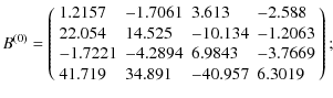
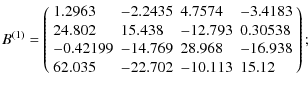
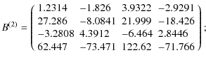
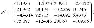
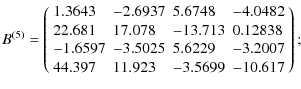
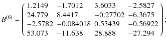
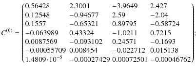
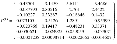
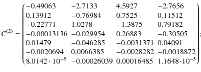
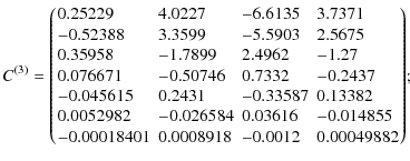
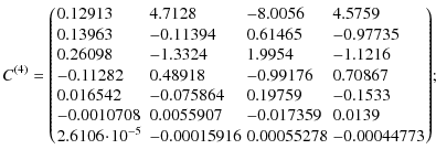
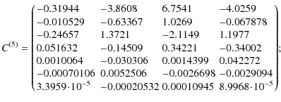
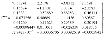
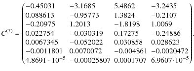
Appendix A: Fitting matrices

The matrices $B^{(\alpha)}$ and $C^{(\alpha)}$ (22), $a = 0, \ldots, M$ contain the coefficients of the reduced-power spectrum fits given in Eq. (21). Here, we provide the numerical values from our fits. The index $\alpha=0$ corresponds to the function Q(12) in the fiducial cosmology, and $\alpha=1, \ldots, 7$ to its derivatives with respect to cosmological parameters (see Table 1). The matrices are also available in electronic form with an example code.

$\displaystyle B^{(0)} = \left( \begin{array}{llll} 1.2157 &-1.7061 &3.613 &-2.5... ...4 &6.9843 &-3.7669 \\ 41.719 &34.891 &-40.957 &6.3019 \\ \end{array}\right) ;$

$\displaystyle B^{(1)} = \left( \begin{array}{llll} 1.2963 &-2.2435 &4.7574 &-3.... ...9 &28.968 &-16.938 \\ 62.035 &-22.702 &-10.113 &15.12 \\ \end{array}\right) ;$

$\displaystyle B^{(2)} = \left( \begin{array}{llll} 1.2314 &-1.826 &3.9322 &-2.9... ...2 &-6.464 &2.8446 \\ 62.447 &-73.471 &122.62 &-71.766 \\ \end{array}\right) ;$

$\displaystyle B^{(3)} = \left( \begin{array}{llll} 1.1772 &-1.523 &3.3478 &-2.6... ...3 &25.431 &-12.429 \\ -1.2271 &192.08 &-259.8 &113.95 \\ \end{array}\right) ;$

$\displaystyle B^{(4)} = \left( \begin{array}{llll} 1.1983 &-1.5973 &3.3941 &-2.... ... &-14.092 &6.4373 \\ 75.097 &-124.48 &200.67 &-109.85 \\ \end{array}\right) ;$

$\displaystyle B^{(5)} = \left( \begin{array}{llll} 1.3643 &-2.6937 &5.6748 &-4.... ... &5.6229 &-3.2007 \\ 44.397 &11.923 &-3.5699 &-10.617 \\ \end{array}\right) ;$

$\displaystyle B^{(6)} = \left( \begin{array}{llll} 1.2149 &-1.7012 &3.6033 &-2.... ...0.53439 &-0.56922 \\ 53.073 &-11.638 &28.888 &-27.294 \\ \end{array}\right) ;$

$\displaystyle B^{(7)} = \left( \begin{array}{llll} 1.3469 &-3.3556 &6.6862 &-4.... ...04 &9.2899 &-4.7514 \\ 37.736 &49.648 &-61.197 &16.44 \\ \end{array}\right) .$

$\displaystyle C^{(0)} = \left(\! \begin{array}{llll} 0.56428 &2.3001 &-3.9649 &... ...}\!\!\! &-0.00027429\! &0.00072501\! &-0.00046762 \\ \end{array}\! \right)\! ;$

$\displaystyle C^{(1)} = \left( \begin{array}{llll} -0.43501 &-3.1459 &5.6111 &-... ...9071 \\ -0.0001238 &0.00098714 &-0.0022652 &0.0014607 \\ \end{array}\right) ;$

$\displaystyle C^{(2)} = \left(\! \begin{array}{llll} -0.49063 &-2.7133 &4.5927 ... ... &-0.00026039 &0.00016485 &1.1648\!\cdot\!10^{-5} \\ \end{array}\! \right)\! ;$

$\displaystyle C^{(3)}=\left(\! \begin{array}{llll} 0.25229 &4.0227 &-6.6135 &3.... ...5 \\ -0.00018401 &0.0008918 &-0.0012 &0.00049882 \\ \end{array}\! \right)\! ;$

$\displaystyle C^{(4)}=\left(\! \begin{array}{llll} 0.12913 &4.7128 &-8.0056 &4.... ...10^{-5} &-0.00015916\! &0.00055278\! &-0.00044773 \\ \end{array}\! \right)\! ;$

$\displaystyle C^{(5)} =\left(\! \begin{array}{llll} -0.31944 &-3.8608 &6.7541 &... ...0.00020532 \! &0.00010945 &8.9968\!\cdot\!10^{-5} \\ \end{array}\! \right)\! ;$

$\displaystyle C^{(6)} =\left(\! \begin{array}{llll} 0.58241 &2.2178 &-3.8312 &2... ...dot\!10^{-5} &-0.00036705 &0.00092519 &-0.0005942 \\ \end{array}\! \right)\! ;$

$\displaystyle C^{(7)}=\left(\! \begin{array}{llll} -0.45031 &-3.1685 &5.4862 &-... ...} &-0.00025807 &0.0001707 &6.9607\!\cdot\!10^{-5} \\ \end{array}\! \right)\! .$

Footnotes

... lensing: Appendix A is only available in electronic form at http://www.aanda.org
... DES: http://www.darkenergysurvey.org
... LSST: http://www.lsst.org
... Euclid: http://www.ias.u-psud.fr/imEuclid
... survey: http://cosmos.astro.caltech.edu
... code: http://www2.iap.fr/users/kilbinge/reduced

All Tables

Table 1: Parameter limits for where the accuracy of the fitted reduced-shear power spectrum is better than $1\%$ for $\ell <10^4$ , and better than $2\%$ for $\ell <2 \times 10^5$ (see also Fig. 3).

All Figures

$\begin{figure} \par\includegraphics[width=8cm,clip]{14829Fg1} \end{figure}$	Figure 1: The function $Q^{(0)}(\ell ) = Q(\ell )$ for different scale factors a as indicated in the panel (points), and the composite fitting function (Eq. (21), lines).
Open with DEXTER
In the text

$\begin{figure} \par\resizebox{18cm}{!}{\includegraphics{14829Fg2}} \end{figure}$	Figure 2: Fit coefficients as a function of scale factor. Left: the polynomial fit coefficients c⁽⁰⁾_i for $i=0, \ldots, N=6$ (Eq. (21)). The lines are polynomials in a or order N_c = 3. Right: the power-law coefficients $b^{(0)}_i, i=0, \ldots, 3$ of the composite function h⁽⁰⁾ (Eq. (18)). The lines are polynomials in a of order N_b = 3.
Open with DEXTER
In the text

$\begin{figure} \par\resizebox{18cm}{!}{\includegraphics{14829Fg3}}\vspace{0.5mm} \vspace{4.25mm} \end{figure}$	Figure 3: The fitted reduced-shear power spectrum (thick lines) and the uncorrected convergence power spectrum (thin lines). Both quantities are plotted as ratios with respect to the reduced-shear power spectrum (6), where the first-order correction $P^{(1)}_{\rm g}$ has been obtained by numerical integration of Eq. (12). In each panel, we show the power spectra at the fiducial model (dashed lines) and the lower (solid) and upper (dashed) boundaries within which a 2% accuracy is reached for $\ell <2 \times 10^5$ , see Table 1.
Open with DEXTER
In the text

Current usage metrics show cumulative count of Article Views (full-text article views including HTML views, PDF and ePub downloads, according to the available data) and Abstracts Views on Vision4Press platform.

Data correspond to usage on the plateform after 2015. The current usage metrics is available 48-96 hours after online publication and is updated daily on week days.

Initial download of the metrics may take a while.