| Issue |
A&A
Volume 522, November 2010
|
|
|---|---|---|
| Article Number | A60 | |
| Number of page(s) | 11 | |
| Section | Celestial mechanics and astrometry | |
| DOI | https://doi.org/10.1051/0004-6361/201014496 | |
| Published online | 03 November 2010 | |
Explicit expansion of the three-body disturbing function for arbitrary eccentricities and inclinations
ASD, IMCCE-CNRS UMR8028, Observatoire de Paris,
UPMC, 77 avenue Denfert-Rochereau,
75014
Paris,
France
e-mail: This email address is being protected from spambots. You need JavaScript enabled to view it.
Received:
24
March
2010
Accepted:
27
June
2010
Abstract
Since the original work of Hansen and Tisserand in the XIXth century, there have been many variations in the analytical expansion of the three-body disturbing function in series of the semi-major axis ratio. With the increasing number of planetary systems of large eccentricity, these expansions are even more interesting as they allow us to obtain for the secular systems finite expressions that are valid for all eccentricities and inclinations. We revisited the derivation of the disturbing function in Legendre polynomial, with a special focus on the secular system. We provide here expressions of the disturbing function for the planar and spatial case at any order with respect to the ratio of the semi-major axes. Moreover, for orders in the ratio of semi-major axis up to ten in the planar case and five in the spatial case, we provide explicit expansions of the secular system, and simple algorithms with minimal computation to extend this to higher order, as well as the algorithms for the computation of non secular terms.
Key words: celestial mechanics / planets and satellites: dynamical evolution and stability / planetary systems / methods: analytical
© ESO, 2010
1. Introduction
In the three-body problem, there are two classical ways to compute the principal part of the disturbing function −Gmm′/Δ. The first approach is to expand it in powers of eccentricity and inclination, with coefficients that are expressed in term of Laplace coefficients (e.g. Laplace 1785; Abu-El-Ata & Chapront 1975; Laskar & Robutel 1995), but this approach, which is well suited to the study of the Solar System, has some limitations for some extra-solar planetary systems, where the eccentricity can reach very high values. Another drawback, is that without some special truncation corrections, the angular momentum will not be conserved exactly in the truncated system.
In the second approach, the expansion is made with respect to the ratio of the semi-major axes of the two bodies α = a/a′, where a′ is related to the external body. Although it may be less efficient for low eccentricity and large values of α, as for the inner planets in the Solar system, the advantage is that this expansion allows us to obtain finite expressions for arbitrary eccentricities in the secular system, while both approaches allow expansions for arbitrary inclinations. The most important contribution to this problem was made in the XIXth century (Hansen 1855; Hill 1875; Tisserand 1899). With the development of space technology, expansions of the disturbing function in term of Legendre polynomials have been rejuvenated for the construction of satellite theories in the vicinity of the Earth (Kozai 1959; Kaula 1962; Brumberg 1967; Brumberg et al. 1971; Giacaglia 1974; Abu-El-Ata & Chapront 1975).
The discovery of new planetary systems, starting with 51Pegb (Mayor & Queloz 1995), has raised the need to revise these methods as many systems have planets with very high eccentricity, as GL 581, HD 217107, HD 69830, HD 74156, HD 168443, HD 102272, HD 169830, HD 202206, HD 183263, or even HD 80606, where the eccentricity reaches 0.931. With the discovery of these numerous new planetary systems, the previous analytical expansions in Laplace coefficients developed for the Solar System are no longer the most appropriate, and we are faced with the need to understand more globally the dynamics of these systems. On the other hand, as the parameters of these extrasolar planetary systems remain not very well known, there is no necessity for very precise analytical approximations. This has led several authors to use the Legendre expansion of the potential for the dynamical study of the secular planetary system, following the previous studies of stellar systems (Krymolowski & Mazeh 1999; Ford et al. 2000; Blaes et al. 2002), where the secular spatial three-body system was expanded up to the octupolar order (α3). In particular, Lee & Peale (2003) used the secular planar system at octupolar order to study the secular dynamics of the HD 168443 and HD 12661 systems. Migaszewski & Goździewski (2008) computed the planar secular system to high order using computer algebra to average over the mean anomaly.
As it appears that there is a growing interest in analytical studies of extra solar planetary systems, we considered it interesting to present a derivation of the planetary (or stellar) disturbing function in a very simple and explicit way that does not already appear in the existing literature. We aimed to write a self-contained paper that allows one to construct explicitly the planetary Hamiltonian to high order, with minimal additional computation. In particular, in Sect. 3 we show that the planar secular system can be obtained explicitly at any order without the need for computer algebra. The spatial case is treated in Sect. 4 with minimal computation when expressed with respect to the mutual inclination J. In the presence of more than two planets, it may be more convenient to use a fixed reference frame, and the derivation of the spatial Hamiltonian is provided in this case in Sect. 4.2. Our derivation is close to the original formulations of Hansen (1855) and Tisserand (1899), but with emphasis on the secular system and the direct derivation of explicit expressions. We also present in Appendix A a new derivation of the Hansen coefficients for the secular terms.
2. Expansion of the disturbing function
To simplify the notations, and although everything can be generalized to an N-body system, we consider here a three-body problem with a central body of mass M and two other celestial bodies of masses m,m′. If we write the Hamiltonian of the Newtonian interactions among these three bodies in Poincaré canonical heliocentric variables, we obtain (Laskar & Robutel 1995, Eq. (15))
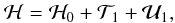 (1)
(1)
where
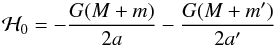 (2)
(2)
is the Keplerian interaction with elliptical elements a,e,i,M,ω, and Ω that denote, respectively, the semi-major axis, eccentricity, inclination, mean anomaly, argument of perihelion, and longitude of the node (with primes for the external body of mass m′). The principal part U1 part of the perturbation and indirect part T1 are then
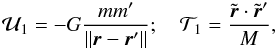 (3)
(3)
where
r,r′
are the radius vectors of the inner and outer planets, with norms
r,r′, unit vectors
u = r/r
and
u′ = r′/r′,
and conjugate momentum  . We focus
first on the principal part of the Hamiltonian U1, which is the most
difficult part to compute, while the computation of the indirect part will be made in
Sect. 5. With
ρ = r/r′,
and
. We focus
first on the principal part of the Hamiltonian U1, which is the most
difficult part to compute, while the computation of the indirect part will be made in
Sect. 5. With
ρ = r/r′,
and  , we have
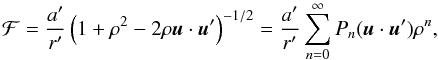 (4)
(4)
where Pn(x) are the Legendre polynomials that can be written as
![Mathematical equation: \begin{equation} P_n(z) = \sum_{k=0}^{[n/2]} p_{n,k}\, z^{n-2k} \end{equation}](/articles/aa/full_html/2010/14/aa14496-10/aa14496-10-eq27.png) (5)
(5)
with
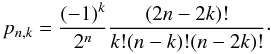 (6)
(6)
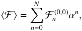
With α = a/a′,γ = r/a,γ′ = r′/a′, we have ρ = αγ/γ′, and thus, as γ,γ′,u,u′ do not depend on a,a′, the expansion of ℱ in powers of α is
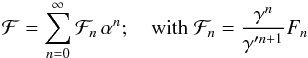 (7)
(7)
and
![Mathematical equation: \begin{equation} F_n=P_n(\uu\dpp\uu')=\sum_{k=0}^{[n/2]} p_{n,k}\, (\uu\dpp\uu')^{n-2k}. \label{eq.fn} \end{equation}](/articles/aa/full_html/2010/14/aa14496-10/aa14496-10-eq36.png) (8)
(8)
3. Planar case
We first study the planar case that leads to some simplifications in the expansions. We define v,v′ to be the true anomalies of u,u′, and ω,ω′ their argument of perihelion, u = v + ω, u′ = v′ + ω′, and x = u − u′. We have then u·u′ = cosx and, following a classical computation (e.g. Whittaker & Watson 1927, p. 303), we have for all z ∈ [ 0,1 [ ,
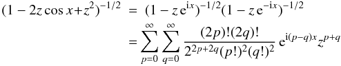 (9)
(9)
and, with n = p + q, and after changing q to n − q,
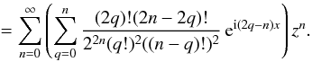 (10)
(10)
Thus
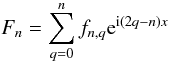 (11)
(11)
with
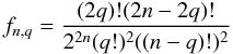 (12)
(12)
for 0 ≤ q ≤ n. If we write x = v − v′ + ω − ω′, ℱn can now be expressed in the form
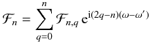 (13)
(13)
with
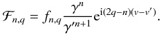 (14)
(14)
The quantities
ℱn,q can then be expressed in term of Hansen coefficients
 defined for n,m ∈ Z as
 (15)
(15)
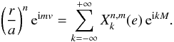
For convenience, we
denote  and
and  . We have thus
 (16)
(16)
For arbitrary values of
k ∈ Z, the Hansen coefficients  can be
expressed in an explicit manner as an infinite series involving Bessel functions and
hypergeometric functions (Hansen 1855; Tisserand 1899), or in terms of generalized Laplace
coefficients (Laskar 2005), but for
k = 0, reduces
to a finite polynomial expression in e,
1/e,
can be
expressed in an explicit manner as an infinite series involving Bessel functions and
hypergeometric functions (Hansen 1855; Tisserand 1899), or in terms of generalized Laplace
coefficients (Laskar 2005), but for
k = 0, reduces
to a finite polynomial expression in e,
1/e,  ,
and
,
and  (see Appendix A). We have thus a very compact expression for the coefficient of any argument
kM + k′M′ in
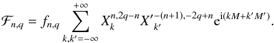
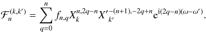
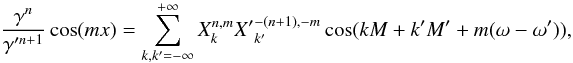
explicit form at all orders n in α. Indeed, if we denote
this coefficient
(see Appendix A). We have thus a very compact expression for the coefficient of any argument
kM + k′M′ in
explicit form at all orders n in α. Indeed, if we denote
this coefficient  , that is
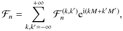 (17)
(17)
we have
 (18)
(18)
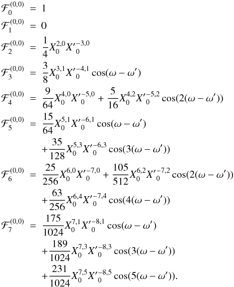
In particular, for all
n ∈ N, the secular part  can even be
simplified, using the classical relation
can even be
simplified, using the classical relation  among Hansen coefficients and
the relation
fn,q = fn,n − q
from Eq. (12)
among Hansen coefficients and
the relation
fn,q = fn,n − q
from Eq. (12)
![Mathematical equation: \begin{eqnarray} % \cF_n^{(0,0)} &=& \epsilon_n f_{n,\frac{n}{2}} X_0^{n,0} {X'}_{0}^{-(n+1), 0} \nonumber \\ \label{eq.perplan} &&\hspace*{-1.2cm} +\sum_{q=0}^{[(n-1)/2]} 2\,f_{n,q} X_0^{n,n-2q} {X'}_{0}^{-(n+1), n-2q} \cos((n-2q)(\om-\om') ), \end{eqnarray}](/articles/aa/full_html/2010/14/aa14496-10/aa14496-10-eq92.png) (19)
(19)
where ϵn = 0 if n is odd, and ϵn = 1 if n is even.
3.1. Practical algorithm
Equations (12) and (19) provide an explicit algorithm for the computation of the principal part of the disturbing function ℱ, and in particular for the computation of the secular Hamiltonian at any order N in α
 (20)
(20)
for which the
involved Hansen coefficients  reduce to finite
expressions (see Appendix A). As there are no secular terms in the indirect part of the
Hamiltonian (see Laskar & Robutel 1995),
the computation of the secular Hamiltonian reduces to the computation of the rational
constants fn,k given by Eq. (12). In practice, for finite order
n, it is even easier to use the expression of
Fn (11) (Table 1) and to translate
it into ℱn (19) by the simple transformation
reduce to finite
expressions (see Appendix A). As there are no secular terms in the indirect part of the
Hamiltonian (see Laskar & Robutel 1995),
the computation of the secular Hamiltonian reduces to the computation of the rational
constants fn,k given by Eq. (12). In practice, for finite order
n, it is even easier to use the expression of
Fn (11) (Table 1) and to translate
it into ℱn (19) by the simple transformation
 (21)
(21)
which
allows an immediate computation of any argument in terms of Hansen
coefficients.
3.2. Computation of the secular part 
The computation of the secular part of the Hamiltonian is quite
simple, as we will just have to make the transformation
 (22)
(22)
in the expression of
Fn. Moreover, we have
 for
m ≥ n ≥ 1 (see Appendix A). The term in cosnx can thus be discarded in the
expression of Fn (Table 1) which simplifies the expression of the Hamiltonian.
The secular Hamiltonian is thus expressed in finite form, using the values of the Hansen
coefficients given in Appendix A. We have
for
m ≥ n ≥ 1 (see Appendix A). The term in cosnx can thus be discarded in the
expression of Fn (Table 1) which simplifies the expression of the Hamiltonian.
The secular Hamiltonian is thus expressed in finite form, using the values of the Hansen
coefficients given in Appendix A. We have
These results are equivalent to the expression obtained by Migaszewski & Goździewski (2008) using computer algebra.
4. Spatial case
The spatial case is more complicated as it involves additional variables. Our goal is to derive explicit formulae that are as compact as possible. We thus expand in terms of the mutual inclination J. For each orbit, we use a reference frame (i,j,k) associated with the orbit, with first vector i in the direction of the ascending node of r′ over r. With u = v + ω and u′ = v′ + ω′, we have
 (23)
(23)
with the same notations as Tisserand (1885)
 (24)
(24)
As in the planar case, we have Fn = Pn(u·u′), but now u·u′ is given by the slightly more complex expression (23). For all n, we have
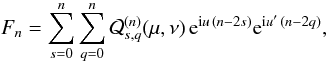 (25)
(25)
where the
 are polynomials in μ,ν of degree
n that are called the Tisserand polynomials2 as a recognition of the work of Tisserand
(1885), although these expressions are already present in (Hansen 1855). As
(u,u′) − → (− u, − u′)
leaves u·u′
unchanged, we have
are polynomials in μ,ν of degree
n that are called the Tisserand polynomials2 as a recognition of the work of Tisserand
(1885), although these expressions are already present in (Hansen 1855). As
(u,u′) − → (− u, − u′)
leaves u·u′
unchanged, we have  , thus
Fn can be expressed as a trigonometric
polynomial in
cos(mu + m′u′).
Although they can be computed explicitly for all n (see Appendix B), for a
given n, it is often more efficient to make a direct computation of
Fn on a computer algebra system. For example,
F20 is computed in less than 1.5 s in exact rational
arithmetics with TRIP (Gastineau & Laskar
2009) on an average laptop computer using the simple expression (8). We can then express
ℱn = (γn/γ′n + 1)Fn
in term of Hansen coefficients. We thus have
, thus
Fn can be expressed as a trigonometric
polynomial in
cos(mu + m′u′).
Although they can be computed explicitly for all n (see Appendix B), for a
given n, it is often more efficient to make a direct computation of
Fn on a computer algebra system. For example,
F20 is computed in less than 1.5 s in exact rational
arithmetics with TRIP (Gastineau & Laskar
2009) on an average laptop computer using the simple expression (8). We can then express
ℱn = (γn/γ′n + 1)Fn
in term of Hansen coefficients. We thus have
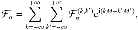 (26)
(26)
with
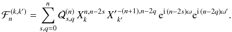 (27)
(27)
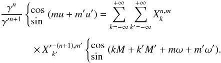
More practically, starting from the finite expressions in cosine polynomials (Table 2) of the Tisserand functions Fn, the expression of ℱn is obtained as in the planar case by means of the more general transformation
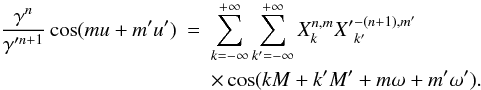 (28)
(28)
4.1. Computation of the secular part
As in the planar case, the computation of the secular part of the Hamiltonian
is just a
straightforward translation of Fn in
Table 2, with the transformation
 (29)
(29)
Moreover, as
 for
n ≥ 1, all terms in
cos(mu ± nu′) can be
discarded in Fn. We thus have,
for
n ≥ 1, all terms in
cos(mu ± nu′) can be
discarded in Fn. We thus have,
![Mathematical equation: \begin{eqnarray*} % \cF_{0}^{(0,0)} \!&=&\!1\nonumber\\ \cF_{1}^{(0,0)} \!&=&\!0\nonumber\\ \cF_{2}^{(0,0)} &=& \left(- \frac{1}{2} + \frac{3}{4} \nu^2 + \frac{3}{4} \mu^2 \right)X_0^{2,0}{X'}_{0}^{-3, 0} \!+ \! \frac{3}{2} \nu \mu X_0^{2,2}{X'}_{0}^{-3, 0} \cos(2\om) \nonumber\\[1mm] \cF_{3}^{(0,0)} &=&X_0^{3,1} {X'}_{0}^{-4,1} \left[ \left(- \frac{3}{2} \mu + \frac{15}{4} \nu^2 \mu + \frac{15}{8} \mu^3 \right) \cos(\om-\om') \right. \nonumber\\[1mm] &&+\left.\left(- \frac{3}{2} \nu + \frac{15}{8} \nu^3 + \frac{15}{4} \nu \mu^2\right) \cos(\om+\om')\right] \nonumber\\[1mm] && +\frac{15}{8}X_0^{3,3} {X'}_{0}^{-4,1} \left[ \nu^2 \mu \cos(3\om+\om') + \nu \mu^2 \cos(3\om-\om')\right]\nonumber\\ % % % \cF_{4}^{(0,0)} &=&X_0^{4,0}{X'}_{0}^{-5, 0}\left( + \frac{3}{8} - \frac{15}{8} \nu^2 \right.\nonumber \\ && \left. + \frac{105}{64} \nu^4 - \frac{15}{8} \mu^2 + \frac{105}{16} \nu^2 \mu^2 + \frac{105}{64} \mu^4\right) \nonumber\\ && + X_0^{4,2}{X'}_{0}^{-5, 2}\left[\left( - \frac{15}{8} \mu^2 \right. \right. \nonumber\\ && \left. + \frac{105}{16} \nu^2 \mu^2 + \frac{35}{16} \mu^4\right) \cos(2\om-2\om') \nonumber \\ &&+\left.\left( - \frac{15}{8} \nu^2 + \frac{35}{16} \nu^4 + \frac{105}{16} \nu^2 \mu^2 \right)\cos(2\om+2\om')\right]\nonumber\\[1mm] && +\left( - \frac{15}{4} \nu \mu + \frac{105}{16} \nu^3 \mu + \frac{105}{16} \nu \mu^3\right) X_0^{4,2}{X'}_{0}^{-5, 0}\cos(2\om) \nonumber\\[1mm] && +\left( - \frac{15}{4} \nu \mu + \frac{105}{16} \nu^3 \mu + \frac{105}{16} \nu \mu^3\right) X_0^{4,0}{X'}_{0}^{-5, 2} \cos(2\om')\nonumber\\[1mm] && +X_0^{4,4}{X'}_{0}^{-5,2}\left[ + \frac{35}{16} \nu \mu^3 \cos(4\om-2\om') \right.\nonumber\\ &&\left. + \frac{35}{16} \nu^3 \mu \cos(4\om+2\om')\right]\nonumber\\ &&+ \frac{105}{32}X_0^{4,4}{X'}_{0}^{-5, 0} \nu^2 \mu^2 \cos(4\om).\nonumber \end{eqnarray*}](/articles/aa/full_html/2010/14/aa14496-10/aa14496-10-eq129.png)
We
thus observe here an important simplification in the quadrupolar secular Hamiltonian
 , as all terms involving
the external planet longitude of perihelion ω′ vanish and we
are left with an integrable Hamiltonian. This is what Lidov & Ziglin (1976) called a happy coincidence (see also Farago & Laskar 2010). This is no longer the
case at higher orders.
, as all terms involving
the external planet longitude of perihelion ω′ vanish and we
are left with an integrable Hamiltonian. This is what Lidov & Ziglin (1976) called a happy coincidence (see also Farago & Laskar 2010). This is no longer the
case at higher orders.
4.2. Expression in a fixed reference frame
Tisserand functions for the spatial case.
Tisserand functions for the spatial case in a fixed reference frame.
The above expressions are given with respect to the mutual inclination to shorten the algebraic expansions. This is especially useful in a three-body problem, but to obtain expressions valid in a fixed reference frame, then one needs to substitute into u·u′ its expression in terms of the elliptical elements of the two bodies. We can then generalize the expression (23) and write it now as (Brumberg 1967; Abu-El-Ata & Chapront 1975; Laskar & Robutel 1995)
 (30)
(30)
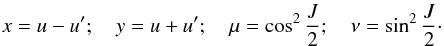
with as before x = u − u′, y = u + u′, and
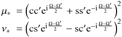 (31)
(31)
with c = cos(i/2), s = sin(i/2), and the same for the primes. We write
 (32)
(32)
with
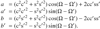 (33)
(33)
With these notations, we have
 (34)
(34)
and
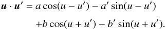 (35)
(35)
The remaining part is identical to the previous case. The expressions of the Tisserand functions Fn are given for 0 ≤ n ≤ 3 in Table 3 and for all n in Appendix B. In practice, for small values of n we can use explicit expressions of Fn, using the straightforward approach consisting of computing Fn directly with computer algebra, using the relation (8), and then to translate it as previously in order to obtain the expression of any argument kM + k′M′ by means of the relations
 (36)
(36)
We
thus have for the secular part ,
![Mathematical equation: \begin{eqnarray*} % \cF_{0}^{(0,0)} &=&1\nonumber\\ \cF_{1}^{(0,0)} &=&0\nonumber\\ \cF_{2}^{(0,0)} &=& X_0^{2,0}{X'}_{0}^{-3, 0}\left[ -\frac{1}{2} +\frac{3}{4}( b'^2 + b^2 + a'^2 + a^2) \right]\nonumber\\ &&\!\!\!\! \!\!\! + \, X_0^{2,2}{X'}_{0}^{-3, 0}\, \frac{3}{2}[ ( b a - b' a') \cos(2 \om) -( b a' + b' a )\sin(2 \om) ]\nonumber % \end{eqnarray*}](/articles/aa/full_html/2010/14/aa14496-10/aa14496-10-eq177.png)
and
![Mathematical equation: \begin{eqnarray*} \cF_{3}^{(0,0)}&=& \frac{15}{8}\nonumber\\ &&\!\!\!\!\!\!\!\!\!\!\!\!\!\!\!\times\, X_0^{3,1}{X'}_{0} ^{-4, 1}\left[+ \left(2 b'^2 a +2 b^2 a + a'^2 a + a^3 -\frac{4}{5} a \right) \cos(\om-\om') \right.\nonumber\\ &&+\, \left(2 b a'^2 +2 b a^2 -\frac{4}{5} b + b'^2 b + b^3 \right)\cos(\om+\om')\nonumber\\ &&+\, \left(\frac{4}{5} b' - b'^3 - b' b^2 -2 b' a'^2 -2b' a^2 \right)\sin(\om+\om')\nonumber\\ &&-\, \left.\left( a' a^2 -\frac{4}{5} a' +2 b'^2 a' +2 b^2 a' + a'^3 \right) \sin(\om-\om')\right]\nonumber\\ &&+\, \frac{15}{8}X_0^{3,3}{X'}_{0}^{-4, 1}[ ( b^2 a -2 b' b a' - b'^2 a )\cos(3 \om+\om')\nonumber\\ &&+\, (b a^2 - b a'^2 -2 b' a' a )\cos(3 \om-\om')\nonumber\\[1mm] &&+\, ( b'^2 a' - b^2 a' -2 b' b a )\sin(3 \om+\om')\nonumber\\[1mm] &&-\, (2 b a' a + b' a^2 - b' a'^2 )\sin(3 \om-\om')] .\nonumber \end{eqnarray*}](/articles/aa/full_html/2010/14/aa14496-10/aa14496-10-eq178.png)
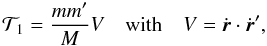
5. Indirect part
Until now, we considered only the principal part of the perturbing Hamiltonian. The computation of the indirect part T1 (3) is more straightforward, as it compares with the computation of r·r′. Indeed, we have (Laskar & Robutel 1995, Eq. (24)),
 (37)
(37)
where
 are the
velocities in the corresponding Keplerian problem. With classical computation, we obtain
are the
velocities in the corresponding Keplerian problem. With classical computation, we obtain
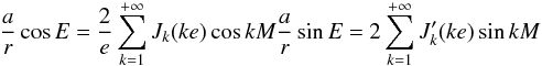 (38)
(38)
where
E is the eccentric anomaly and
Jk(x) are the Bessel
functions. The coordinates (Ẋ,Ẏ) of the
velocity
 in the
reference frame of the orbit with origin at perihelion are then easily expressed in Fourier
series of the mean anomaly, as
in the
reference frame of the orbit with origin at perihelion are then easily expressed in Fourier
series of the mean anomaly, as
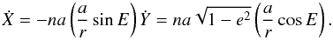 (39)
(39)
If we denote 𝒵 = Ẋ + iẎ, we then have for the spatial problem in the fixed reference frame, with the same notations as in the previous section (Laskar & Robutel 1995, Eq. (37)),
 (40)
(40)
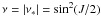
If one considers the mutual inclination J, as in Sect. 4, this expression simplifies since Ω = Ω′, s′ = 0, c′ = 1, and μ * ,ν * are then real, with μ * = cos2(J/2), ν * = sin2(J/2). In the planar case (Sect. 3), μ * = 1, ν * = 0.
We considered here heliocentric coordinates. One could also use Jacobi coordinates for the three-body problem. In this case, the indirect part does not require additional computations as it is expressed in term of u·u′ (see Laskar 1990). It should be noted that in terms of both heliocentric coordinates or Jacobi coordinates, the indirect part does not contribute to the secular system. We have provided here the expression of the indirect part for the computation of non-secular inequalities.
6. Conclusion
We have presented a self-contained exposition of the expansion of the three-body Hamiltonian in canonical heliocentric coordinates in term of Legendre polynomials at any order in the ratio of semi-major axes α, which can also be adapted in the case of Jacobi coordinates, where only the indirect part differs. We have included here all the necessary material that allows one to write explicitly the secular Hamiltonian at order α10 for the planar case, α5 for the spatial case expressed in terms of the mutual inclination, and α3 for the spatial case in a fixed reference frame. With the additional computation of the required Hansen coefficients, the expressions of the Tisserand functions Fn can also be used for a straightforward computation of the expression of a non-secular inequality kM + k′M′.
As the algorithms that are presented here are very simple, we have not added to this paper any tables in electronic form. Indeed, the reader who needs to use expressions of high order that do not appear in the paper, will have no problems in exploiting the algorithms given here to derive the required expressions. The written results of the paper can then be used to check his computations for the lowest orders. For example, the computation of F100, in the spatial case takes less than 8 min on an average 8 core desktop computer in exact rational arithmetics using TRIP, but has 2 343 926 terms, while F50 needs only 7.5 s with already 164 151 terms. As the algorithms require only a few lines of code (fewer than 20 in our case), one understands that it is preferable to compute the terms when they are needed than to store the values in electronic form.
One should consult (Aksenov 1986) for a detailed discussion of the relation between the Tisserand polynomials and the inclination functions of Kaula (1962).
Appendix A: Computation of the Hansen coefficients
 is
the polynomial part of the Hansen coefficients
is
the polynomial part of the Hansen coefficients  .
.
Hansen coefficients  for
(0 ≤ n ≤ 10,0 ≤ m ≤ n).
for
(0 ≤ n ≤ 10,0 ≤ m ≤ n).
The Hansen coefficients  are defined as the Fourier coefficients
 (A.1)
(A.1)
For arbitrary
values of k ∈ Z, the Hansen coefficients can be expressed in an explicit manner as an
infinite series involving Bessel functions and hypergeometric functions (Hansen 1855; Hill
1875; Tisserand 1899), or generalized
Laplace coefficients (Laskar 2005), but for
k = 0, reduces to a simple polynomial in
e, 1/e,  ,
and
,
and  .
The literature on the computation of the Hansen coefficients has been huge since the
original work of Hansen (1855), but we do not
review it here. We concentrate on the obtention of the coefficients
.
The literature on the computation of the Hansen coefficients has been huge since the
original work of Hansen (1855), but we do not
review it here. We concentrate on the obtention of the coefficients
 and
and  , for n ≥ 0 and
0 ≤ m ≤ n that are required to compute the averaged
planetary or lunar Hamiltonian. Using
, for n ≥ 0 and
0 ≤ m ≤ n that are required to compute the averaged
planetary or lunar Hamiltonian. Using
 (A.2)
(A.2)
where v is the true anomaly and E the eccentric anomaly, we have for n ≥ 2
![Mathematical equation: \appendix \setcounter{section}{1} \begin{eqnarray} X_0^{-n,m} &=& \frac{1}{\sqrt{1-e^2}} \frac{1}{2\pi}\int_0^{2\pi} \left(\frac{a}{r}\right)^{n-2} \e^{\i mv} {\rm d}v \nonumber \\[2mm] &=&\frac{1}{(1-e^2)^{n-3/2}} \frac{1}{2\pi}\int_0^{2\pi} (1+e\cos v)^{n-2} \e^{\i mv} {\rm d}v\nonumber \\[2mm] &=&\frac{1}{(1-e^2)^{n-3/2}} \nonumber \\[2mm] &&\times \sum_{l=0}^{[(n-2-m)/2]}\!\!\!\!\! \frac{(n-2)!}{l!\,(m+l)!\,(n-2-(m+2l))!} \left(\frac{e}{2}\right)^{m+2l} \cdot \label{eq.anomv} \end{eqnarray}](/articles/aa/full_html/2010/14/aa14496-10/aa14496-10-eq352.png) (A.3)
(A.3)
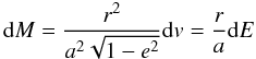
We still need to consider the case n = 1 for which the expansion in true anomaly v is not suitable. We have immediately, using (A.6)
 (A.4)
(A.4)
It is important to note that from (A.3), we have
 (A.5)
(A.5)
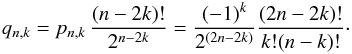
The Hansen
coefficients  are given in
Table A.1 for n ≥ 2 and
m ≤ n − 2. On the other hand, the computation of
are given in
Table A.1 for n ≥ 2 and
m ≤ n − 2. On the other hand, the computation of
 for n ≥ 0 is not as
straightforward, as a direct expansion of
for n ≥ 0 is not as
straightforward, as a direct expansion of
![Mathematical equation: \appendix \setcounter{section}{1} \begin{eqnarray} X_0^{n,m} &= & \frac{1}{2\pi}\int_0^{2\pi} \left(\frac{r}{a}\right)^{n+1} \e^{\i mv} {\rm d}E \nonumber \\[2mm] &=& \frac{1}{2\pi}\int_0^{2\pi} (1-e\cos E)^{n+1-m} (\cos E -e\nonumber \\[2mm] && +\, {\rm i}\sqrt{1-e^2}\sin E)^m {\rm d}E \label{eq.anomE} \end{eqnarray}](/articles/aa/full_html/2010/14/aa14496-10/aa14496-10-eq360.png) (A.6)
(A.6)
in
eccentric anomaly is far more complicated than the previous expression (A.3). One can still perform some formal
expansion, but this would not be very useful, as it would contain expressions with many
summations that cannot be easily reduced to a single summation as in (A.3). In fact, the only explicit computation
of available in the literature, was obtained
through a complex process in (Hansen 1855; Hill 1875; Tisserand
1899), using the auxiliary variable 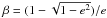 . In this case, it can be
shown that is expressed as a finite hypergeometric series
in β2. Using a relation among hypergeometric series due to
Gauss, and the change of variable
e = 2β/(1 + β2),
Tisserand (1899) provides a finite expression of
in term of hypergeometric series of
e2. We present here a more direct demonstration for the
obtention of an explicit expression of which is a recurrence using the relation among
Hansen coefficients
. In this case, it can be
shown that is expressed as a finite hypergeometric series
in β2. Using a relation among hypergeometric series due to
Gauss, and the change of variable
e = 2β/(1 + β2),
Tisserand (1899) provides a finite expression of
in term of hypergeometric series of
e2. We present here a more direct demonstration for the
obtention of an explicit expression of which is a recurrence using the relation among
Hansen coefficients
 (A.7)
(A.7)
This relation appears in
(Hughes 1981), but it was shown by Laskar (2005) that it is equivalent to a recurrence
relation obtained on Laplace coefficients by Laplace
(1785). The computation of  for
n ≥ 0 using (A.6) is
straightforward and gives
for
n ≥ 0 using (A.6) is
straightforward and gives
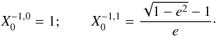
![Mathematical equation: \appendix \setcounter{section}{1} \begin{equation} X_0^{n,0} = \sum_{l=0}^{[(n+1)/2]} \frac{(n+1)!}{l!\,l!\,(n+1-2l)!} \left(\frac{e}{2}\right)^{2l}\cdot \end{equation}](/articles/aa/full_html/2010/14/aa14496-10/aa14496-10-eq367.png) (A.8)
(A.8)
The computation of
 can also be performed
using (A.6). Changing E
to − E, it is immediate to see that the part in sinE
cancel, and we are left with
can also be performed
using (A.6). Changing E
to − E, it is immediate to see that the part in sinE
cancel, and we are left with
![Mathematical equation: \appendix \setcounter{section}{1} \begin{equation} X_0^{n,1} =- (n+2)\sum_{l=0}^{[n/2]} \frac{n!}{l!\,(l+1)!\,(n-2l)!} \left(\frac{e}{2}\right)^{2l+1}\cdot \end{equation}](/articles/aa/full_html/2010/14/aa14496-10/aa14496-10-eq371.png) (A.9)
(A.9)
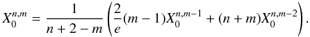
We can now prove by
recurrence using the relation (A.7) that
the general form of  for n ≥ 0
and 0 ≤ m ≤ n is
for n ≥ 0
and 0 ≤ m ≤ n is
![Mathematical equation: \appendix \setcounter{section}{1} \begin{eqnarray} X_0^{n,m} &=&(-1)^m \frac{(n+ 1+m)!}{(n+1)!} \nonumber\\[2.5mm] &&\times \sum_{l=0}^{[(n+1-m)/2]} \frac{(n+1-m)!}{l!\,(m+l)!\,(n+1- m-2l)!} \left(\frac{e}{2}\right)^{m+2l}\cdot \label{eq.xnm} \end{eqnarray}](/articles/aa/full_html/2010/14/aa14496-10/aa14496-10-eq373.png) (A.10)
(A.10)
The
computation is delicate but straightforward. One can first show that the two first
elements (for l = 0) of the polynomial expressions of
 and
and
 in (A.7) cancel. We then change the index from
l to l + 1 and show that the general term of the sum
in (A.7) gives the general term of
in (A.7) cancel. We then change the index from
l to l + 1 and show that the general term of the sum
in (A.7) gives the general term of
 , and that the last term of
will give the
last term of . The expression (A.10) is equivalent to the expression of
(Tisserand 1899).The expressions of the Hansen
coefficients are given in Table A.2 for 0 ≤ n ≤ 10 and
0 ≤ m ≤ n.
, and that the last term of
will give the
last term of . The expression (A.10) is equivalent to the expression of
(Tisserand 1899).The expressions of the Hansen
coefficients are given in Table A.2 for 0 ≤ n ≤ 10 and
0 ≤ m ≤ n.
Appendix B: Computation of Tisserand polynomials and Tisserand functions
Expansions valid for all inclinations were already given by Hansen (1855), and Tisserand (1885) in his researches on asteroidal motions, but these derivations are rather complex. Although in (B.3) we present some of Tisserand’s computations, we make first, as in the planar case some direct expansions and reordering of terms to obtain expressions that are as compact as possible.
B.1. Tisserand functions with respect to mutual inclination
With x = u − u′, y = u + u′, μ = cos2(J/2), ν = sin2(J/2), we have
 (B.1)
(B.1)
and with a straightforward expansion in complex notation, we obtain
 (B.2)
(B.2)
which we can reorder as
 (B.3)
(B.3)
with
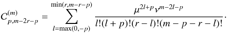 (B.4)
(B.4)
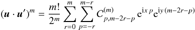
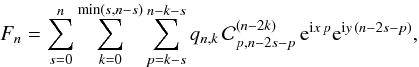
With the expansion (8), we have then
![Mathematical equation: \appendix \setcounter{section}{2} \begin{equation} F_n = \sum_{k=0}^{[n/2]} q_{n,k}\, \sum_{r=0}^{n-2k} \sum_{p=-r}^{n-2k-r} \cC_{p,n-2k-2r-p}^{(n-2k)}\, \e^{\i x\,p}\e^{\i y\,(n-2k-2r-p)} \label{eq.fkrp} \end{equation}](/articles/aa/full_html/2010/14/aa14496-10/aa14496-10-eq389.png) (B.5)
(B.5)
with
 (B.6)
(B.6)
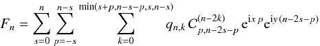
We can then reorder (B.5) with s = k + r as
 (B.7)
(B.7)
exchange the sum in p and k
 (B.8)
(B.8)
and set q = p + s which gives
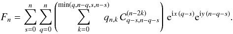 (B.9)
(B.9)
That is, with x = u − u′ and y = u + u′,
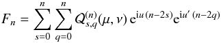 (B.10)
with
 (B.11)
that is
 (B.12)
B.2. Tisserand functions with respect to a fixed reference frame
In the case of a fixed reference frame (Sect. 4.2), the expressions differ slightly, but are more complicated. We have (35)
 (B.13)
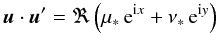
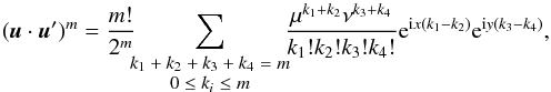
that is, with μ * = a + ia′, ν * = b + ib′,
![Mathematical equation: \appendix \setcounter{section}{2} \begin{equation} \uu\dpp\uu' = \frac{1}{2}\left[ \tmu \e^{\i x} + \bmus \e^{-\i x}+ \tnu \e^{\i y} + \bnus \e^{-\i y}\right]. \end{equation}](/articles/aa/full_html/2010/14/aa14496-10/aa14496-10-eq405.png) (B.14)
(B.14)
This is similar to the previous expression (B.1), and the computation of the Tisserand functions Fn will follow the same lines and gives the more general expression
 (B.15)
with
 (B.16)
The
coefficients  (B.12) and
  (B.16) in the Tisserand functions are very similar. Indeed, using
μ = 1 − ν and
(B.16) in the Tisserand functions are very similar. Indeed, using
μ = 1 − ν and  (34), we have
 (B.17)
with
 and
and
 (B.18)
B.3. Tisserand simplification
The above expression (B.18) is a double sum. In the mutual inclination case, Tisserand (1885) could reduce it to a single sum using hypergeometric functions. He first considers the differential equation satisfied by Legendre polynomials
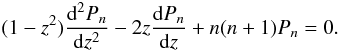 (B.19)
As Fn = Pn(z) (Eq. (8)) with z = cosx + ν(cosy − cosx) (Eq. (B.1)), we have from (B.19),
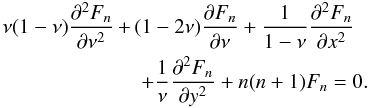 (B.20)
Using expressions (B.10, B.17), one then replaces Fn in (B.20) by
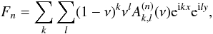 (B.21)
which leads to
 (B.22)
where
![Mathematical equation: \appendix \setcounter{section}{2} \begin{eqnarray} \cA^{(n)}_{k,l}(\nu) &=& \nu(1-\nu)\frac{{\rm d}^2A^{(n)}_{k,l}}{{\rm d}\nu^2} +\big[1+2l-2(k+l+1)\nu\big]\frac{{\rm d}A^{(n)}_{k,l}}{{\rm d}\nu} \nonumber\\ &&+\,(n-k-l)(n+k+l+1)A^{(n)}_{k,l}. \label{eq.diffAn} \end{eqnarray}](/articles/aa/full_html/2010/14/aa14496-10/aa14496-10-eq422.png) (B.23)
(B.23)
The
equality (B.22) must be satisfied for all
x and y, thus all the coefficients
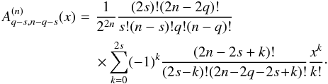
 (B.23) are equal to 0. The solutions of (B.23) are
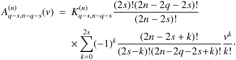
 (B.24)
or equivalently
 (B.25)
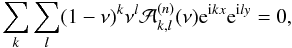
where
 is an unknown
constant and F an hypergeometric function (e.g. Whittaker & Watson 1927). Let us assume that the quantity
2n − 2q − 2s + 1 is positive. If it
is not the case, one can make the change of variable
(s,q) → (n − s′,n − q′).
Then
2n − 2q′ − 2s′ + 1
is positive and since Fn is real,
is an unknown
constant and F an hypergeometric function (e.g. Whittaker & Watson 1927). Let us assume that the quantity
2n − 2q − 2s + 1 is positive. If it
is not the case, one can make the change of variable
(s,q) → (n − s′,n − q′).
Then
2n − 2q′ − 2s′ + 1
is positive and since Fn is real,
 (B.10). From (B.25), one thus has
 (B.26)
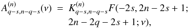
Tisserand (1885) needs then some lengthy computations
to determine from the
coefficient of νn in
Fn. Here, we use the expression (B.12) with (B.17) and (B.26). With
μ = 1 − ν, we get
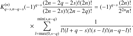 (B.27)
Calculating the coefficient of the term xs in (1 + x)n − q(1 + x)q = (1 + x)n, one finds
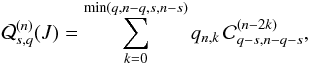
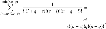 (B.28)
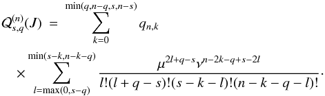
Thus, from (B.27), we obtain
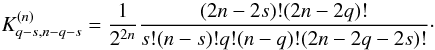 (B.29)
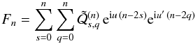
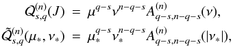
Finally, the most general case, where inclinations are defined with respect to a fixed reference plane, can be as well derived from (B.17) and (B.29). We have
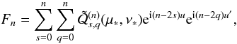 (B.30)
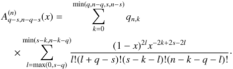
where
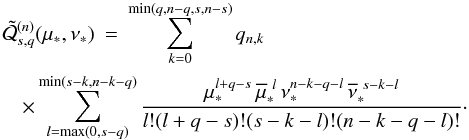
![Mathematical equation: \appendix \setcounter{section}{2} \begin{equation} \tilde{\cQ}^{(n)}_{s,q}(\tmu,\tnu) = \left\{ \begin{array}{ll} \tmu^{q-s}\,\tnu^{n-q-s}A^{(n)}_{q-s,n-q-s}(\abs{\tnu}) & \textrm{if } s+q\leq n , \\[1mm] \bmus^{\ s-q}\,\bnus^{\ s+q-n}A^{(n)}_{s-q,s+q-n}(\abs{\tnu}) & \textrm{else}, \end{array} \right. \label{eq.Qtilde} \end{equation}](/articles/aa/full_html/2010/14/aa14496-10/aa14496-10-eq442.png) (B.31)
(B.31)
and
 (B.32)
In
(B.31), we used the fact that
 is the complex
conjugate of
is the complex
conjugate of  since
Fn is real.
since
Fn is real.
References
- Abu-El-Ata, N., & Chapront, J. 1975, A&A, 38, 57 [NASA ADS] [Google Scholar]
- Aksenov, E. P. 1986, SvA, 30, 221 [NASA ADS] [Google Scholar]
- Blaes, O., Lee, M. H., & Socrates, A. 2002, ApJ, 578, 775 [NASA ADS] [CrossRef] [Google Scholar]
- Brumberg, V. A. 1967, Bull. Inst. Theor. Astron., XI, 73 [Google Scholar]
- Brumberg, V. A., Evdokimova, L. S., & Kochina, N. G. 1971, Celest. Mech., 3, 197 [Google Scholar]
- Farago, F., & Laskar, J. 2010, MNRAS, 401, 1189 [NASA ADS] [CrossRef] [Google Scholar]
- Ford, E. B., Kozinsky, B., & Rasio, F. A. 2000, ApJ, 535, 385 [NASA ADS] [CrossRef] [Google Scholar]
- Gastineau, M., & Laskar, J. 2009, TRIP 1.0, TRIP Reference manual, IMCCE, Paris Observatory, http://www.imcce.fr/Equipes/ASD/trip/trip.html [Google Scholar]
- Giacaglia, G. E. O. 1974, Celest. Mech., 9, 239 [NASA ADS] [CrossRef] [Google Scholar]
- Hansen, P. 1855, Abhandl. d. K. S. Ges. d. Wissensch, IV, 182 [Google Scholar]
- Hill, G. W. 1875, The Analyst, II, 161 [CrossRef] [Google Scholar]
- Hughes, S. 1981, Celest. Mech., 25, 101 [NASA ADS] [CrossRef] [Google Scholar]
- Kaula, W. M. 1962, AJ, 67, 300 [NASA ADS] [CrossRef] [Google Scholar]
- Kozai, Y. 1959, AJ, 64, 367 [NASA ADS] [CrossRef] [MathSciNet] [Google Scholar]
- Krymolowski, Y., & Mazeh, T. 1999, MNRAS, 304, 720 [NASA ADS] [CrossRef] [Google Scholar]
- Laplace, P. 1785, in Oeuvres Complètes, T11 (Paris: Gauthier-Villars) [Google Scholar]
- Laskar, J. 1990, in Les Méthodes Modernes de la Mécanique Céleste, ed. C. F. D. Benest [Google Scholar]
- Laskar, J. 2005, Celest. Mech. Dynam. Astron., 91, 351 [NASA ADS] [CrossRef] [Google Scholar]
- Laskar, J., & Robutel, P. 1995, Celest Mech. Dynam. Astron., 62, 193 [Google Scholar]
- Lee, M. H., & Peale, S. J. 2003, ApJ, 592, 1201 [NASA ADS] [CrossRef] [Google Scholar]
- Lidov, M. L., & Ziglin, S. L. 1976, Celest. Mech., 13, 471 [NASA ADS] [CrossRef] [Google Scholar]
- Mayor, M., & Queloz, D. 1995, Nature, 378, 355 [NASA ADS] [CrossRef] [Google Scholar]
- Migaszewski, C., & Goździewski, K. 2008, MNRAS, 388, 789 [NASA ADS] [CrossRef] [Google Scholar]
- Tisserand, F. 1885, Annales de l’Observatoire de Paris, 18, 1 [Google Scholar]
- Tisserand, F. 1899, Traité de Mécanique Céleste (Paris: Gauthier-Villars) [Google Scholar]
- Whittaker, E., & Watson, G. 1927, A course of modern analysis (Cambridge University Press) [Google Scholar]
All Tables
Current usage metrics show cumulative count of Article Views (full-text article views including HTML views, PDF and ePub downloads, according to the available data) and Abstracts Views on Vision4Press platform.
Data correspond to usage on the plateform after 2015. The current usage metrics is available 48-96 hours after online publication and is updated daily on week days.
Initial download of the metrics may take a while.