| Issue |
A&A
Volume 539, March 2012
|
|
|---|---|---|
| Article Number | A35 | |
| Number of page(s) | 11 | |
| Section | Astrophysical processes | |
| DOI | https://doi.org/10.1051/0004-6361/201117871 | |
| Published online | 22 February 2012 | |
Mean-field transport in stratified and/or rotating turbulence
1 NORDITA, AlbaNova University Center, Roslagstullsbacken 23, 10691 Stockholm, Sweden
e-mail: This email address is being protected from spambots. You need JavaScript enabled to view it.
2 Department of Astronomy, AlbaNova University Center, Stockholm University, 10691 Stockholm, Sweden
3 Astrophysical Institute Potsdam, An der Sternwarte 16, 14482 Potsdam, Germany
Received: 10 August 2011
Accepted: 4 January 2012
Abstract
Context. The large-scale magnetic fields of stars and galaxies are often described in the framework of mean-field dynamo theory. At moderate magnetic Reynolds numbers, the transport coefficients defining the mean electromotive force can be determined from simulations. This applies analogously also to passive scalar transport.
Aims. We investigate the mean electromotive force in the kinematic framework, that is, ignoring the back-reaction of the magnetic field on the fluid velocity, under the assumption of axisymmetric turbulence determined by the presence of either rotation, density stratification, or both. We use an analogous approach for the mean passive scalar flux. As an alternative to convection, we consider forced turbulence in an isothermal layer. When using standard ansatzes, the mean magnetic transport is then determined by nine, and the mean passive scalar transport by four coefficients. We give results for all these transport coefficients.
Methods. We use the test-field method and the test-scalar method, where transport coefficients are determined by solving sets of equations with properly chosen mean magnetic fields or mean scalars. These methods are adapted to mean fields which may depend on all three space coordinates.
Results. We find the anisotropy of turbulent diffusion to be moderate in spite of rapid rotation or strong density stratification. Contributions to the mean electromotive force determined by the symmetric part of the gradient tensor of the mean magnetic field, which were ignored in several earlier investigations, turn out to be important. In stratified rotating turbulence, the α effect is strongly anisotropic, suppressed along the rotation axis on large length scales, but strongly enhanced at intermediate length scales. Also the  effect is enhanced at intermediate length scales. The turbulent passive scalar diffusivity is typically almost twice as large as the turbulent magnetic diffusivity. Both magnetic and passive scalar diffusion are slightly enhanced along the rotation axis, but decreased if there is gravity.
Conclusions. The test-field and test-scalar methods provide powerful tools for analyzing transport properties of axisymmetric turbulence. Future applications are proposed ranging from anisotropic turbulence due to the presence of a uniform magnetic field to inhomogeneous turbulence where the specific entropy is nonuniform, for example. Some of the contributions to the mean electromotive force which have been ignored in several earlier investigations, in particular those given by the symmetric part of the gradient tensor of the mean magnetic field, turn out to be of significant magnitude.
Key words: magnetohydrodynamics (MHD) / hydrodynamics / turbulence / Sun: dynamo
© ESO, 2012
1. Introduction
Stellar mixing length theory is a rudimentary description of turbulent convective energy transport. The mixing length theory of turbulent transport goes back to Prandtl (1925) and, in the stellar context, to Vitense (1953). The simplest form of turbulent transport is turbulent diffusion, which quantifies the mean flux of a given quantity, e.g., momentum, concentration of chemicals, specific entropy or magnetic fields, down the gradient of its mean value. In all these cases essentially a Fickian diffusion law is established, where the turbulent diffusion coefficient is proportional to the rms velocity of the turbulent eddies and the effective mean free path of the eddies or their correlation length.
Mean-field theories, which have been elaborated, e.g., for the behavior of magnetic fields or of passive scalars in turbulent media, go beyond this concept. In the case of magnetic fields, the effects of turbulence occur in a mean electromotive force, which is related to the mean magnetic field and its derivatives in a tensorial fashion. Examples for effects described by the mean magnetic field alone, without spatial derivatives, are the α-effect (Steenbeck et al. 1966) and the pumping of mean magnetic flux (Rädler 1966, 1968; Roberts & Soward 1975); for more information on these topics see, e.g., Krause & Rädler (1980) or Brandenburg & Subramanian (2005). Likewise the mean passive scalar flux contains a pumping effect (Elperin et al. 1996). In both the magnetic and the passive scalar cases turbulent diffusion occurs, which is in general anisotropic. The coupling between the mean electromotive force and the magnetic field and its derivatives, or mean passive scalar flux and the mean scalar and its derivatives, is given by turbulent transport coefficients.
On the analytic level of the theory the determination of these transport coefficients is only possible with some approximations. The most often used one is the second-order correlation approximation (SOCA), which has delivered so far many important results. Its applicability is however restricted to certain ranges of parameters like the magnetic Reynolds number or the Péclet number. In spite of this restriction, SOCA is an invaluable tool, because it allows a rigorous treatment within the limits of its applicability. It is in particular important for testing numerical methods that apply in a wider range.
In recent years it has become possible to compute the full set of turbulent transport coefficients numerically from simulations of turbulent flows. The most accurate method for that is the test-field method (Schrinner et al. 2005, 2007). In addition to the equations describing laminar and turbulent flows, one solves a set of evolution equations for the small-scale magnetic or scalar fields which result from given mean fields, the test fields. By selecting a sufficient number of independent test fields, one obtains a corresponding number of mean electromotive forces or mean scalar fluxes and can then compute in a unique way all the associated transport coefficients.
Most of the applications of the test-field method are based on spatial averages that are taken over two coordinates. In the magnetic case this approach has been applied to a range of different flows including isotropic homogeneous turbulence (Sur et al. 2008; Brandenburg et al. 2008a), homogeneous shear flow turbulence (Brandenburg et al. 2008b) without and with helicity (Mitra et al. 2009), and turbulent convection (Käpylä et al. 2009). One of the main results is that in the isotropic case, for magnetic Reynolds numbers Rm larger than unity, the turbulent diffusivity is given by  , where the correlation time τ is, to a good approximation, given by τ = (urmskf)-1. Here, urms is the rms velocity of the turbulent small-scale flow and kf is the wavenumber of the energy-carrying eddies. For smaller Rm, the turbulent diffusivity grows linearly with Rm. Furthermore, if the turbulence is driven isotropically by polarized waves, the flow becomes helical and there is an α effect. In the kinematic regime (for weak magnetic fields), the α coefficient is proportional to
  , where ω = ∇ × u is the vorticity of the small-scale flow, u. In the passive scalar case, test scalars are used to determine the transport coefficients. Results have been obtained for anisotropic flows in the presence of rotation or strong magnetic fields (Brandenburg et al. 2009), linear shear (Madarassy & Brandenburg 2010), and for irrotational flows (Rädler et al. 2011).
The present paper deals with the magnetic and the passive scalar case in the above sense. Its goal is to compute the transport coefficients for axisymmetric turbulence, that is, turbulence with one preferred direction, given by the presence of either rotation or density stratification or, if the relevant directions coincide, of both. (Axisymmetric turbulence can be defined by requiring that any averaged quantity depending on the turbulent velocity field is invariant under any rotation of this field about the preferred axis.) Note that a dynamo-generated magnetic field will in general violate the assumption of axisymmetric turbulence. To avoid this problem while still being able to investigate the general effects arising from only one preferred direction, we assume such fields to be weak so as not to affect the assumption of axisymmetry of the turbulence. An imposed uniform magnetic field in the preferred direction would still be allowed, but this case will not be investigated in this paper; see Brandenburg et al. (2009) for numerical investigations of passive scalar transport with a uniform field.
Except for a few comparison cases, we always consider flows in a slab between stress-free boundaries. This is the simplest example of flows that are non-vanishing on the boundary and compatible with axisymmetric turbulence. To facilitate comparison with earlier work on forced turbulence, we consider an isothermal layer even in the density-stratified case, i.e., there is no convection, and the flow is driven by a prescribed random forcing. This is similar to earlier work on forced homogeneous turbulence (Brandenburg et al. 2008a,b, 2009), but now we will be able to address questions regarding vertical pumping as well as helicity production and α effect in the presence of rotation. This setup allows us to isolate effects of density stratification from those originating from the nonuniformities of turbulence intensity and local correlation length. In addition to isothermal stratification, we assume an isothermal equation of state and thus do not consider an equation for the specific entropy. Hence, no Brunt-Väisälä oscillations can occur. This assumption would need to be relaxed for studying turbulent convection, which will be the subject of a future investigation.
2. Mean-field concept in turbulent transport
2.1. Mean electromotive force
The evolution of the magnetic field B in an electrically conducting fluid is assumed to obey the induction equation, 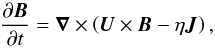 (1)where U is the velocity and η the microscopic magnetic diffusivity of the fluid, and J is defined by J = ∇ × B (so that J/μ0 with μ0 being the magnetic permeability is the electric current density). We define mean fields as averages, assume that the averaging satisfies (exactly or approximately) the Reynolds rules, and denote averaged quantities by overbars1. The mean magnetic field
  is then governed by
 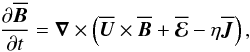 (2)where
  is the mean electromotive force resulting from the correlation of velocity and magnetic field fluctuations,
  and
and  .
.
We focus attention on the mean electromotive force  in cases in which the velocity fluctuations u constitute axisymmetric turbulence, that is, turbulence with one preferred direction, which we describe by the unit vector
  . Until further notice we accept the traditional assumption according to which in a given point in space and time is a linear homogeneous function of and its first spatial derivatives in this point. Then, can be represented in the form
 ![Mathematical equation: \begin{eqnarray} \meanEMF&=& -\alpha_\perp\meanBB -(\alpha_\parallel-\alpha_\perp)(\eee\cdot\meanBB)\eee -\gamma\eee\times\meanBB \nonumber \\[2mm] &&-\beta_\perp\meanJJ -(\beta_\parallel-\beta_\perp)(\eee\cdot\meanJJ)\eee -\delta\eee\times\meanJJ \label{eq005}\\[2mm] &&-\kappa_\perp\meanKK -(\kappa_\parallel-\kappa_\perp)(\eee\cdot\meanKK)\eee -\mu\eee\times\meanKK \nonumber \end{eqnarray}](/articles/aa/full_html/2012/03/aa17871-11/aa17871-11-eq27.png) (3)with nine coefficients α ⊥ , α ∥ , ..., μ2. Like
(3)with nine coefficients α ⊥ , α ∥ , ..., μ2. Like  , also
  is determined by the gradient tensor
  . While
  is given by its antisymmetric part, is a vector defined by
  with
with  being the symmetric part of . A more detailed explanation of (3) is given in Appendix A. If is understood as polar vector (for example
  , where
  is the mean mass density), then is axial and γ, β⊥, β∥ and μ are true scalars, but α⊥, α∥, δ, κ⊥ and κ∥ pseudoscalars. (Scalars are invariant but pseudoscalars change sign if the turbulent velocity field is reflected at a point or at a plane containing the preferred axis.) Sometimes it is useful to interpret as an axial vector (for example Ω/|Ω| with Ω being an angular velocity). Then, is a polar vector, β⊥, β∥, δ, κ⊥, κ∥ and μ are true scalars but α⊥, α∥ and γ pseudoscalars.
We may split and into parts  and
and  perpendicular to and parts
  and
and  parallel to it. Then (3) can be written in the form
 ![Mathematical equation: \begin{eqnarray} \meanEMF_\perp &=& -\alpha_\perp \meanBB_\perp -\gamma\eee \times \meanBB_\perp -\beta_\perp \meanJJ_\perp -\delta \eee \times \meanJJ_\perp \nonumber\\[2.5mm] &\quad-&\kappa_\perp \meanKK_\perp -\mu \eee \times \meanKK_\perp \label{eq007}\\[2.5mm] \meanEMF_\parallel &=& - \alpha_\parallel \meanBB_\parallel -\beta_\parallel \meanJJ_\parallel -\kappa_\parallel \meanKK_\parallel. \nonumber \end{eqnarray}](/articles/aa/full_html/2012/03/aa17871-11/aa17871-11-eq52.png) (4)Let us return to (3). In the simple case of homogeneous isotropic turbulence we have α⊥ = α∥ and β ⊥ = β∥, and all remaining coefficients vanish. Then, (3) takes the form
(4)Let us return to (3). In the simple case of homogeneous isotropic turbulence we have α⊥ = α∥ and β ⊥ = β∥, and all remaining coefficients vanish. Then, (3) takes the form  with properly defined α and ηt. These two coefficients have been determined by test-field calculations (Sur et al. 2008; Brandenburg et al. 2008a).
In several previous studies of , more general kinds of turbulence (that is, not only axisymmetric turbulence) have been considered, but with a less general definition of mean fields, which were just horizontal averages. More precisely, Cartesian coordinates (x,y,z) were adopted and the averages were taken over all x and y so that they depend on z and t only (Brandenburg et al. 2008a,b). This definition implies remarkable simplifications. Of course, we then have  . Further, there are no non-zero components of other than
  and
and  , for
, for  requires
  , and these components can be expressed as components of , viz.
  and
and  . (Here and in what follows, commas denote partial derivatives.) This again implies
  . As a consequence, this definition of mean fields reduces (3) to
 ![Mathematical equation: \begin{eqnarray} \meanEMF &=& - \alpha_{\perp} \meanBB - (\alpha_{\parallel}-\alpha_{\perp})(\eee \cdot \meanBB) \eee - \gamma \eee \times \meanBB \nonumber\\[2.5mm] \label{eq011} && -\beta^{\dag} \meanJJ - \delta^{\dag} \, \eee \times \meanJJ, \end{eqnarray}](/articles/aa/full_html/2012/03/aa17871-11/aa17871-11-eq70.png) (5)where and . Of course, α ⊥ , α ∥ , γ, and are independent of x or y. Clearly, β ⊥ and μ as well as δ and κ ⊥ have no longer independent meanings. From (2) we may conclude that
(5)where and . Of course, α ⊥ , α ∥ , γ, and are independent of x or y. Clearly, β ⊥ and μ as well as δ and κ ⊥ have no longer independent meanings. From (2) we may conclude that  . If we restrict ourselves to applications in which
  vanishes initially, it does so at all times and the term with α ∥ − α ⊥ in (5) disappears. Then, only the four coefficients α ⊥ , γ, and are of interest. They can be determined by test-field calculations using two test fields independent of x and y (Brandenburg et al. 2008a,b).
In this paper we go beyond the aforementioned assumptions in the following respects. Firstly, we relax the assumption that in a given point in space is a homogeneous function of and its first spatial derivatives in this point. Instead, we admit a non-local connection between and . For simplicity, however, we further on assume that at a given time depends only on at the same time, that is, we remain with an instantaneous connection between and . This approximation requires that the mean field varies slowly on a time scale much longer than the turnover time of the turbulence; see Hubbard & Brandenburg (2009) for a more general treatment of rapidly changing fields. Secondly, we consider mean fields no longer as averages over all x and y. We define at a point (x,y) in a plane z = const by averaging over some surroundings of this point in this plane so that it still depends on x and y. In that sense we generalize (3) so that 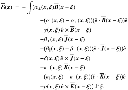 (6)As a consequence of the axisymmetry of the turbulence, the coefficients α ⊥ , α ∥ , ..., μ depend only via
  on ξx and ξy. We consider them also as symmetric in ξz. The integration is over all ξ space. Of course, , , , and may depend on t. For simplicity, however, the argument t has been dropped.
Let us subject (6) to a Fourier transformation with respect to ξ. We define it by 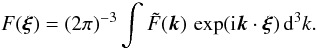 (7)Remembering the convolution theorem we obtain
 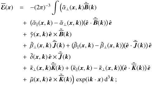 (8)see Chatterjee et al. (2011) for a corresponding relation in the case of horizontally averaged magnetic fields that depend only on z. Like α⊥, α∥, ..., μ, the
  ,
,  , ...,
  are real quantities. They depend only via
  on kx and ky and are symmetric in kz, i.e., depend only via k∥ = |kz| on kz. Due to the reality of the α ⊥ , α∥, ..., μ and their symmetry in ξx, ξy and ξz we have
 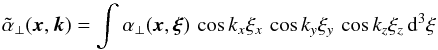 (9)and analogous relations for , ..., . We note that , ..., , taken at k = 0, agree with α⊥, ..., μ in Eq. (3).
2.2. Mean passive scalar flux
There are interesting analogies between turbulent transport of magnetic flux and that of a passive scalar (cf. Rädler et al. 2011). Assume that the evolution of a passive scalar C, e.g., the concentration of an admixture in a fluid, is given by 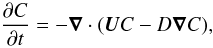 (10)where D is the microscopic (molecular) diffusivity. Then the mean scalar
  has to satisfy
 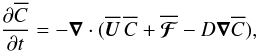 (11)where
  is the mean passive scalar flux, u stands again for the fluctuations of the velocity and
  for the fluctuations of C. Consider again axisymmetric turbulence with a preferred direction given by the unit vector . Assume that
  in a given point in space and time is determined by and its gradient
  in this point. Then we have
  (12)with coefficients γC,
  ,
,  and δC. If is a polar vector, γC is a scalar but δC a pseudoscalar, and if is an axial vector, γC is a pseudoscalar but δC a scalar, while and are always scalars. We note that
  is only unequal zero if δC is not constant but varies in the direction of
  .
.
We may split and  into parts
  and
and  perpendicular to , and parts
  and
and  parallel to it, and give (12) the form
 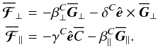 (13)Let us now relax the assumption that in a given point in space and time is determined by and in this point. Analogously to the magnetic case we consider a non-local but instantaneous connection between and . Then we have
 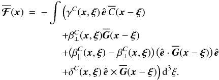 (14)As α⊥, α∥, ..., μ in the magnetic case, γC, , and δC depend only via on ξx and ξy, and we consider them also as symmetric in ξz. The integration is again over all ξ space. Note that , , and may, even if it is not explicitly indicated, depend on t. Applying the Fourier transformation defined by (7) on (14), we arrive at
 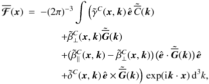 (15)where
  ,
,  ,
,  and
and  are real quantities. They depend only via
  on kx and ky, and only via k∥ on kz, and they satisfy relations analogous to (9). We note that
  , , , and at k = 0 agree with γC, ,
  , and δC in (12).
3. Simulating the turbulence
We assume that the fluid is compressible and its flow is governed by the equations 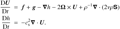 (16)Here, f means a random force which primarily drives isotropic turbulence (e.g., Haugen et al. 2004), g the gravitational force, and h the specific enthalpy. An isothermal equation of state,
  , has been adopted with a constant isothermal sound speed cs. In general a fluid flow in a rotating system is considered, Ω is the angular velocity which defines the Coriolis force. As usual ρ means the mass density, ν the kinematic viscosity and S the trace-free rate of strain tensor,
 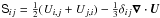 . The influence of the magnetic field on the fluid motion, that is the Lorentz force, is ignored throughout the paper.
The numerical simulation is carried out in a cubic domain of size L3, so the smallest wavenumber is k1 = 2π/L. In most of the cases a density stratification is included with g = (0,0, −g), so the density scale height is  . The number of scale heights across the domain is equal to Δlnρ, where Δ denotes the difference of values at the two edges of the domain. The forcing is assumed to work with an average wavenumber kf. The scale separation ratio is then given by kf/k1, for which we usually adopt the value 5. This means that we have about 5 eddies in each of the three coordinate directions.
The flow inside the considered domain depends on the boundary conditions. Unless indicated otherwise we take the top and bottom surfaces z = z1 and z = z2 with z2 = −z1 = L/2 as stress-free and adopt periodic boundary conditions for the other surfaces.
4. Computing the transport coefficients
4.1. Test-field method
In the magnetic case the coefficients α⊥, α∥, ..., μ are determined by the test-field method (Schrinner et al. 2005, 2007; Brandenburg et al. 2008a). This method works with a set of test fields , called  , and the corresponding mean electromotive forces , called
  . For the latter we have
  , where the bT obey
 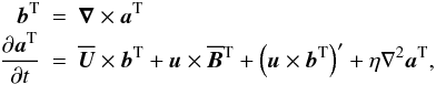 (17)with
  and u taken from the solutions of (16). For the boundaries z = const we choose conditions which correspond to an adjacent perfect conductor, for the x and y directions periodic boundary conditions.
We define four test fields by 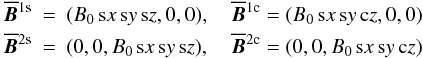 (18)with a constant B0. Here and in what follows we use the abbreviations
 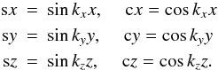 (19)We recall that test-fields need not to be solenoidal (see Schrinner et al. 2005, 2007).
We denote the mean electromotive forces which correspond to the test fields (18) by  ,
,  ,
,  , and
, and  . With the presentation (6) and relations like (9) we find
 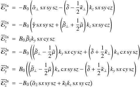 (20)and corresponding relations for
  , whose right-hand sides can be derived from those in (20) simply by replacing sz and cz by cz and − sz, respectively.
In view of the assumed axisymmetry of the turbulence, we consider α⊥, α∥, ..., μ in what follows as independent of x and y but admit a dependence on z. When multiplying both sides of Eqs. (20) and of the corresponding ones for with sx sy, sx cy or cy sy and averaging over all x and y, we obtain a system of equations, which can be solved for , , ..., . The result reads 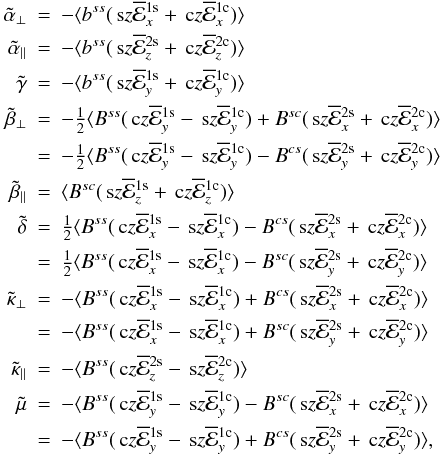 (21)where
 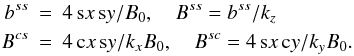 (22)The angle brackets indicate averaging over x and y. Although the relations (21) and (22) contain kx, ky and kz as independent variables, the , , ..., should vary only via with kx and ky, and only via k ∥ with kz.
4.2. Test-scalar method
In the passive-scalar case the coefficients γC, , , and δC are determined by the test-scalar method with test scalars  and the corresponding fluxes
  . For the latter, we have
  , where cT obeys
 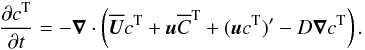 (23)Again and u are taken from the solutions of (16).
We define two test-scalars  and
and  by
by  (24)where C0 is a constant and the abbreviations (19) are used. From (14) we then have
 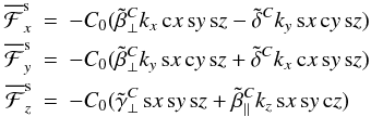 (25)and analogous relations for
  with sz and cz replaced by cz and − sz, respectively.
Analogous to the magnetic case, we assume that γC, , , and δC are independent of x and y but may depend on z. Analogous to (21) we find here 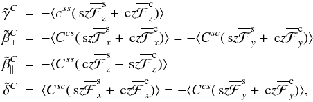 (26)where css, Css, Csc, and Ccs are defined like bss, Bss, Bsc, and Bcs, with C0 at the place of B0. The angle brackets indicate again averaging over x and y. Note that , , , and should depend only via on kx and ky, and only via k∥ on kz.
4.3. Validation using the Roberts flow
For a validation of our test-field procedure for the determination of the coefficients occurring in (3) we rely on the Roberts flow. We define it here by 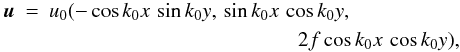 (27)with some wavenumber k0 and a factor f which characterizes the ratio of the magnitude of uz to that of ux and uy. We further define mean fields as averages over x and y with an averaging scale which is much larger than the period length 2π/k0 of the flow pattern. When calculating the mean electromotive force for this flow, we assume that it is a linear homogeneous function of and its first spatial derivatives and adopt the second-order correlation approximation. Although the Roberts flow is far from being axisymmetric, the result for can be written in the form (3), and we have
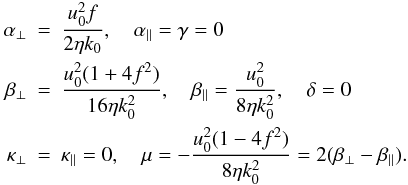 (28)It agrees with and can be deduced from results reported in Rädler et al. (2002a,b). As for the passive scalar case, an analogous analytical calculation of the mean scalar flow
  leads to (12) with
 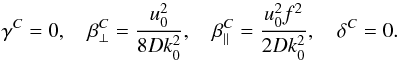 (29)We may proceed from the local connection of with and its derivatives considered in (3) to the non-local ones given by (6) or (8). As a consequence of the deviation of the flow from axisymmetry, we can then no longer justify that coefficients like α ⊥ (ξ) depend only via on ξx and ξy, and coefficients like
  only via k ⊥ on kx and ky. This applies analogously to the connection of with and its derivatives and to coefficients like β ⊥ (ξ) and
  .
.
A test-field calculation of the coefficients , , ..., , as well as , ..., , has been carried out under the conditions of the second-order correlation approximation with u given by (27) and f = 1/ . Figure 1 shows the results obtained for ,
  ,
,  and , as well as
  and
and  , as functions of k ⊥ /kf, with
  , for two fixed ratios k∥/k⊥. In the limit k⊥/kf ≪ 1 these coefficients take just the values of α⊥, β⊥, β∥, μ, and given in (28) and (29). For larger values of k⊥/kf, as to be expected, the , , , , and depend also on the ratio of kx and ky.
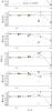 |
Fig. 1 The coefficients |
4.4. Dimensionless parameters and related issues
Within the framework of this paper, the coefficients α⊥, α∥, ..., μ as well as , , ..., , and likewise γC, , ..., δC and , , ..., , have to be considered as functions of several dimensionless parameters. In the magnetic case these are the magnetic Reynolds number Rm = urms/ηkf and the magnetic Prandtl number Pm = ν/η, in the passive scalar case the Péclet number Pe = urms/Dkf and the Schmidt number Sc = ν/D, further the Mach number Ma = urms/cs, the gravity parameter  , the Coriolis number Co = 2Ω/urmskf, as well as the scale separation ratio kf/k1.
Throughout the rest of the paper we give the coefficients α ⊥ , α∥, γ, and γC as well as , ,  , and in units of urms/3, the remaining coefficients β⊥, ..., δC and , ..., in units of urms/3kf. The numerical calculations deliver these coefficients as functions of z and t. To avoid boundary effects, we average these results over −2 ≤ k1z ≤ 1 (see Fig. 3 below). The resulting time series are averaged over a range where the results are statistically stationary, i.e., there is no trend in the time series. Error bars are defined by comparing the maximum departure of an average over any one third of the time series with the full time average.
In the case of isotropic turbulence it has been observed that many of the transport coefficients enter an asymptotic regime as soon as Rm exceeds unity (Sur et al. 2008). While this should be checked in every new case again (see below), it is important to realize that, according to several earlier results (see also Brandenburg et al. 2009), only values of Rm below unity are characteristic of the diffusively dominated regime, while for Rm exceeding unity the transport coefficients turn out to be nearly independent of the value of Rm.
We are often interested in the limit k ⊥ ,k∥ → 0, in which the , , ... turn into the α ⊥ , α∥...δC. In this limit, however, the test fields and test scalars defined by (18) and (24) vanish. Unless specified otherwise, we approach this limit by choosing the smallest possible non-zero |kx|, |ky| and |kz|, that is, by putting kx = ky = kz = k1.
In the figures of the next section results for , , ... are represented. In all cases in which they are considered as results for the limit k⊥,k∥ → 0 they are simply denoted as α⊥, α∥...δC in the text.
5. Results
5.1. Homogeneous rotating turbulence
Let us first consider homogeneous turbulence in a rotating system, that is, under the influence of the Coriolis force. The angular velocity Ω responsible for this force defines the preferred direction of the turbulence,  . In this case we expect only contributions to the mean electromotive force from a spatially varying mean magnetic field , and contributions to the passive scalar flux from a spatially varying mean passive scalar . That is, in (3) we have only the terms with β⊥, β∥, δ, κ⊥, κ∥, and μ, and in (12) only those with
  , , and δC. The terms with β⊥ and β∥, as well as those with and , characterize anisotropic mean-field diffusivities, and that with δ corresponds to the “
 effect” (Rädler 1969a,b, 1976; Krause & Rädler 1971, 1980; Rädler et al. 2003), while the δC term vanishes underneath the divergence and is therefore without interest.
Figure 2 shows the dependence of the aforementioned coefficients on Co for Rm ≈ Pe ≈ 9 and kf/k1 = 5. The values of β⊥, β∥, and , which remain finite for Co → 0, are always close together. The other four coefficients vary linearly with Co as long as Co is small. Specifically, we find  ,
,  , as well as
  and
and  . These coefficients reach maxima at Co ≈ 1. For rapid rotation, |Co| ≫ 1, all coefficients approach zero like 1/Co. In particular, we have β ⊥ ≈ 1.2/Co and the same for β ∥ , , and , further
  ,
,  ,
,  , and
, and  . Furthermore, we find that, within error bars, α⊥, α∥, γ, and γC are indeed zero.
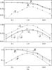 |
Fig. 2 Co dependence of transport coefficients in a model with rotation but zero density stratification, Rm ≈ 9, Pm = Sc = 1, Gr = 0, kf/k1 = 5. |
5.2. Stratified turbulence
Owing to the presence of boundary conditions at the top and bottom of our domain and the lack of scale separation for our default choice of kf/k1 = 5, the turbulence is in all cases anisotropic, even if gravity is negligible. The ratio of the vertical and horizontal velocity components,  , is no longer, as in the isotropic case, equal to unity. For moderate stratification (
 ), not too large |z|, and kf/k1 = 5, it takes a value of about 0.9. It decreases when the ratio kf/k1 is decreased; see Table 1. Figure 3 shows the z dependence of . For strong stratification and a high degree of scale separation, e.g. kf/k1 = 30, the mentioned ratio comes close to unity. Note, however, that smaller values of
  can be can be achieved in the non-isothermal case when the effects of buoyancy become important.
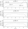 |
Fig. 3 Anisotropy |
5.2.1. Stratified nonrotating turbulence
For axisymmetric turbulence in a nonrotating system showing any kind of stratification in the representation (3) of only the four coefficients γ, β ⊥ , β∥, and μ can be non-zero. Likewise, in the representation (12) of only the three coefficients γC, , and can be non-zero. Figure 4 shows their dependence on Gr. It appears that γ is always close to zero, while γC shows a linear increase for not too strong gravity. At the same time, β ⊥ , β∥, , and remain approximately constant. We find that μ is negative and its modulus is mildly increasing with increasing stratification, but the error bars are large.
Dependence of the density contrast ρbot/ρtop and the degree of anisotropy , for three different values of kf/k1, on the density stratification  for nonrotating turbulence.
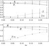 |
Fig. 4 Gr dependence of the transport coefficients in a model with density stratification but zero rotation, Pm = Sc = 1, Rm ≈ 22, Co = 0, kf/k1 = 5. |
5.2.2. Stratified rotating turbulence
For turbulence under the influence of gravity and rotation, all nine coefficients α ⊥ , ..., μ are in general non-zero, as well as all four coefficients γC, ..., δC. If both gravity and rotation are so small that is linear in g and Ω, more precisely contains gmΩn, where n and m mean integers, only with n + m ≤ 1, α⊥ and α∥ vanish but γ, β⊥, δ and κ⊥ may well be unequal to zero. If n + m ≤ 2, all nine coefficients may indeed be non-zero.
Results for stratified rotating turbulence are shown in Fig. 5. The error bars are now bigger than either with just rotation or just stratification. For Co → 0, the coefficients β⊥, β∥, μ, , and δC remain finite. As Co is increased, their moduli show some decline. On the other hand the moduli of α⊥, α∥, γ, δ, κ⊥, κ∥ and γC increase with Co as long as it is smaller than some value below unity but decrease again for larger Co. Both α⊥ and α∥ are negative, which is expected for g and Ω being antiparallel to each other. Interestingly, μ is finite for small values of Co, in agreement with the result when there is only stratification (Fig. 4), but with a modest amount of rotation, μ is suppressed and grows only when Co has reached values around unity.
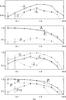 |
Fig. 5 Co dependence of transport coefficients in a model with rotation and density stratification, Pm = Sc = 1, Rm ≈ 10, Gr ≈ 0.16, kf/k1 = 5. |
5.3. Wavenumber dependence
So far we have considered the coefficients , , ..., in the limit k = |k| → 0, that is, k ⊥ ,k ∥ → 0. However, their behavior for larger k, in particular for k up to several kf, is of interest, too. Most of them decrease like k-2 as k grows and can be fitted to a Lorentzian profile, as has been found in earlier calculation using the test-field method; see Brandenburg et al. (2008a), where in fact the dependence on k ∥ was considered. Even earlier work that was not based on the test-field method showed a declining trend (Miesch et al. 2000; Brandenburg & Sokoloff 2002). Nevertheless, as is shown in Fig. 6, there are also some coefficients that first increase with k ∥ , have a maximum near k ∥ = kf and only then decrease with growing k ∥ . Examples for such a behavior are ,  , and
, and  , while
  peaks slightly below k∥ = 0.5kf.
The dependence of the coefficients under discussion on k⊥ is shown in Fig. 7. Note that our test fields vanish for k⊥ = 0, so no values are shown for this case. Note also that  ,
,  , and
, and  , which have maxima for k∥/kf ≈ 1 or k∥/kf ≈ 0.5, show a clear monotonic decline with k ⊥ . Only
  has maxima with respect to both k∥/kf and k ⊥ /kf.
Most of the results presented in Fig. 7 have been calculated with kx = ky, a few single ones for , , and also with kx/ky = 0.75 and kx/ky = 0.2. While the results for and agree well for all these values of kx/ky, there are significant discrepancies with and .
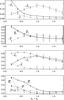 |
Fig. 6 k∥ dependence of transport coefficients in a model with rotation and density stratification, |

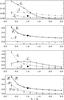 |
Fig. 7 Same as Fig. 6, but k⊥ dependence, k∥ = k1. The filled and open circles denote results for α⊥, β⊥, κ⊥, and |
5.4. Dependencies on Rm and Pe
Let us finally consider the dependence of all transport coefficients on Rm or Pe for a case where they are all expected to be finite. Therefore we choose again the case with Co = 1 and Gr = 0.16, which was also considered in Figs. 5–7, and keep Pm = Sc = 1.
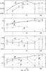 |
Fig. 8 Dependencies of the transport coefficients on Rm or Pe in a model with rotation and density stratification, Pm = Sc = 1, Co = 1.0, Gr = 0.16, kf/k1 = 5. |
The results are shown in Fig. 8. As expected, some of the quantities increase approximately linearly with Rm if Rm < 1, or with Pe if Pe < 1, and seem to level off to constant values for larger values of Rm, or Pm, although the uncertainty tends to increase significantly.
6. Conclusions
In this paper we have dealt with the mean electromotive force and the mean passive scalar flux in axisymmetric turbulence and have calculated the transport coefficients that define these quantities. Unlike most of the earlier work, we have no longer assumed that mean fields are defined as planar averages but admit a dependence on all three space coordinates. The number of test fields and test scalars is the same (4 and 2, respectively) as in earlier work using planar averages, so the computational cost is unchanged.
We may conclude from general symmetry considerations that the mean electromotive force has altogether nine contributions: three defined by the mean magnetic field , three by the mean current density , and three by the vector , which is the projection of the symmetric part of the gradient tensor of the magnetic field on the preferred direction. In many representations of the last three contributions have been ignored. Our results underline that this simplification is in general not justified. The corresponding coefficients κ⊥, κ∥ and μ are in general not small compared to β⊥, β∥ and δ.
It has been known since long that a stratification of the turbulence intensity, that is, a gradient of  , causes a pumping of magnetic flux (Rädler 1966, 1968, 1969b). It remained however uncertain whether the same effect occurs if a preferred direction is given by a gradient of the mean mass density while the turbulence intensity is spatially constant. In our calculations, which correspond to this assumption, the value of γ is not clearly different from zero. This suggests that a gradient of the mass density alone is not sufficient for pumping, what is also in agreement with results of Brandenburg et al. (2011). This is even more remarkable as the corresponding coefficient γC which describes the transport of a mean passive scalar is noticeably different from zero. Pumping down the density gradient is indeed expected (Elperin et al. 1995). An explanation of these results would be very desirable.
In homogeneous rotating turbulence, apart from an anisotropy of the mean-field conductivity, the effect occurs (Rädler 1969a,b). In the passive scalar case again an anisotropy of the mean diffusivity is possible. Even if the flux proportional to  is non-zero, it cannot influence .
Let us turn to the induction effects described by . If the preferred direction is given by a polar vector, the corresponding contribution to the mean electromotive force can only be proportional to  . We found such a contribution in the case of the Roberts flow and also, for turbulence subject the Coriolis force, in the results presented in Figs. 2 and 4–7.
Contributions to the mean electromotive force as described here by occur also in earlier calculations, e.g. Kitchatinov et al. (1994) or Rüdiger & Brandenburg (1995). As a consequence of other notations, however, this is not always obvious. For example, Rüdiger & Brandenburg (1995) consider a mean electromotive force of the form  (30)with two coefficients η ∥ and ηT (Eq. (18) of their paper with
  , in the sense of the definition introduced here, replaced by ;
  is our ). It is equivalent to our representations (3) or (4) of if we put there
  , β∥ = ηT, μ = η∥ − ηT and all other coefficients equal to zero. This implies β⊥ − β∥ = μ/2, which is in agreement with the relation for μ in Eq. (28) for the Roberts flow. The latter equality is also approximately obeyed for turbulence in the presence of rotation, stratification, and both; see Figs. 2, 4 and 5, respectively.
If there is moderate rotation (Co ≈ 1), but no stratification, we have β⊥ > β∥; see Fig. 2. This means, e.g., that for a magnetic field without a component in the direction of the rotation axis the diffusion along this axis is enhanced compared with that in the perpendicular direction. In the passive scalar case we have  , which implies that the diffusion along the rotation axis is enhanced, too. However, stratification enlarges β∥ − β⊥ and diminishes
  so that the diffusion along the rotational axis is decreased in both cases considered. In the presence of rotation and density stratification all three contributions to the mean electromotive force described by are in general non-zero. Here, |κ⊥| is smaller than |κ∥|. There is now also an α effect, which is necessarily anisotropic, and |α∥| is typically only half as big as |α⊥|; see Fig. 5.
The present work is applicable to investigations of stellar convection either with or without rotation, and it would provide a more comprehensive description of turbulent transport properties than what has been available so far (Käpylä et al. 2009). The methods utilized in this paper can be extended to a large class of phenomena in which turbulence with just one preferred direction plays an important role. Examples for that include turbulence under the influence of a strong magnetic field and/or an externally applied electric field leading to a current permeating the system. Turbulence generated by the Bell (2004) instability is an example. In addition to density stratification, there can be a systematic variation of the turbulence intensity in one direction. A further example is entropy inhomogeneity combined with gravity giving rise to Brunt-Väisälä oscillations. Pumping effects also exist in homogeneous flows if the turbulence is helical (Mitra et al. 2009; Rogachevskii et al. 2011). By contrast, shear problems or other types of problems with two or more preferred directions that are inclined to each other (e.g., turbulence in a local domain of a rotating stratified shell at latitudes different from the two poles) are not amenable to such a study. Of course, although we refer here to axisymmetric turbulence, problems in axisymmetric cylindrical geometry are also not amenable to this method, because the turbulence must be homogeneous in one plane.
The Reynolds rules imply that  ,
,  ,
,  ,
,  and
and  for any fluctuating quantities F and G.
Note that the signs in front of some individual terms on the right-hand side of (3), in particular of those with α⊥ and α∥ (perpendicular and parallel α effect) as well as γ (pumping in the z direction), may differ from the signs used in other representations.
Acknowledgments
A.B. and K.-H.R. are grateful for the opportunity to work on this paper while participating in the program “The Nature of Turbulence” at the Kavli Institute for Theoretical Physics in Santa Barbara, CA. This work was supported in part by the European Research Council under the AstroDyn Research Project No. 227952 and by the National Science Foundation under Grant No. NSF PHY05-51164. We acknowledge the allocation of computing resources provided by the Swedish National Allocations Committee at the Center for Parallel Computers at the Royal Institute of Technology in Stockholm and the National Supercomputer Centers in Linköping.
References
- Bell, A. R. 2004, MNRAS, 353, 550 [Google Scholar]
- Brandenburg, A., & Sokoloff, D. 2002, Geophys. Astrophys. Fluid Dyn., 96, 319 [NASA ADS] [CrossRef] [Google Scholar]
- Brandenburg, A., & Subramanian, K. 2005, Phys. Rep., 417, 1 [NASA ADS] [CrossRef] [Google Scholar]
- Brandenburg, A., Rädler, K.-H., & Schrinner, M. 2008a, A&A, 482, 739 [NASA ADS] [CrossRef] [EDP Sciences] [Google Scholar]
- Brandenburg, A., Rädler, K.-H., Rheinhardt, M., & Käpylä, P. J. 2008b, ApJ, 676, 740 [NASA ADS] [CrossRef] [Google Scholar]
- Brandenburg, A., Svedin, A., & Vasil, G. M. 2009, MNRAS, 395, 1599 [NASA ADS] [CrossRef] [Google Scholar]
- Brandenburg, A., Kemel, K., Kleeorin, N., & Rogachevskii, I. 2011, ApJ, submitted [Google Scholar]
- Chatterjee, P., Mitra, D., Rheinhardt, M., & Brandenburg, A. 2011, A&A, 534, A46 [NASA ADS] [CrossRef] [EDP Sciences] [Google Scholar]
- Elperin, T., Kleeorin, N., & Rogachevskii, I. 1995, Phys. Rev. Lett., 52, 2617 [NASA ADS] [Google Scholar]
- Elperin, T., Kleeorin, N., & Rogachevskii, I. 1996, Phys. Rev. Lett., 76, 224 [NASA ADS] [CrossRef] [Google Scholar]
- Haugen, N. E. L., Brandenburg, A., & Dobler, W. 2004, Phys. Rev. E, 70, 016308 [NASA ADS] [CrossRef] [Google Scholar]
- Hubbard, A., & Brandenburg, A. 2009, ApJ, 706, 712 [NASA ADS] [CrossRef] [Google Scholar]
- Käpylä, P. J., Korpi, M. J., & Brandenburg, A. 2009, A&A, 500, 633 [NASA ADS] [CrossRef] [EDP Sciences] [Google Scholar]
- Kitchatinov, L. L., Rüdiger, G., Pipin, V. V., & Rüdiger, G. 1994, Astron. Nachr., 315, 157 [NASA ADS] [CrossRef] [Google Scholar]
- Krause, F., & Rädler, K.-H., 1971, in Ergebnisse der Plasmaphysik und der Gaselektronik Band 2, ed. R. Rompe, & M. Steenbeck (Berlin: Akademie-Verlag), 6 [Google Scholar]
- Krause, F., & Rädler, K.-H. 1980, Mean-Field Magnetohydrodynamics and Dynamo Theory (Berlin, Pergamon, Cambridge: Akademie-Verlag Press) [Google Scholar]
- Madarassy, E. J. M., & Brandenburg, A. 2010, Phys. Rev. E, 82, 016304 [NASA ADS] [CrossRef] [Google Scholar]
- Miesch, M. S., Brandenburg, A., & Zweibel, E. G. 2000, Phys. Rev. E, 61, 457 [Google Scholar]
- Mitra, D., Käpylä, P. J., Tavakol, R., & Brandenburg, A. 2009, A&A, 495, 1 [NASA ADS] [CrossRef] [EDP Sciences] [Google Scholar]
- Prandtl, L. 1925, Zeitschr. Angewandt. Math. Mech., 5, 136 [Google Scholar]
- Rädler, K.-H. 1966, Thesis Univ. Jena [Google Scholar]
- Rädler, K.-H. 1968, Z. Naturforschg., 23a, 1851 [Google Scholar]
- Rädler, K.-H. 1969a, Mber. Dt. Akad. Wiss, 11, 194 [Google Scholar]
- Rädler, K.-H. 1969b, Geod. Geophys. Veröffentlichungen Reihe II Heft, 13, 131 [Google Scholar]
- Rädler, K.-H. 1976, in Basic Mechanisms of Solar Activity, ed. V. Bumba, & J. Kleczek (Dordrecht: D. Reidel Publishing Company), 323 [Google Scholar]
- Rädler, K.-H., Rheinhardt, M., Apstein, E., & Fuchs, H. 2002a, Magnetohydrodynamics, 38, 39 [Google Scholar]
- Rädler, K.-H., Rheinhardt, M., Apstein, E., & Fuchs, H. 2002b, Nonlinear Process. Geophys., 9, 171 [Google Scholar]
- Rädler, K.-H., Kleeorin, N., & Rogachevskii, I. 2003, Geophys. Astrophys. Fluid Dyn., 97, 249 [Google Scholar]
- Rädler, K.-H., Brandenburg, A., Del Sordo, F., & Rheinhardt, M. 2011, Phys. Rev., E84, 046321 [NASA ADS] [Google Scholar]
- Roberts, P. H., & Soward, A. M. 1975, Astron. Nachr., 296, 49 [NASA ADS] [CrossRef] [Google Scholar]
- Rogachevskii, I., Kleeorin, N., Käpylä, P. J., & Brandenburg, A. 2011, Phys. Rev. E, 84, 056314 [NASA ADS] [CrossRef] [Google Scholar]
- Rüdiger, G., & Brandenburg, A. 1995, A&A, 296, 557 [NASA ADS] [Google Scholar]
- Schrinner, M., Rädler, K.-H., Schmitt, D., Rheinhardt, M., & Christensen, U. 2005, Astron. Nachr., 326, 245 [NASA ADS] [CrossRef] [Google Scholar]
- Schrinner, M., Rädler, K.-H., Schmitt, D., Rheinhardt, M., & Christensen, U. R. 2007, Geophys. Astrophys. Fluid Dyn., 101, 81 [NASA ADS] [CrossRef] [MathSciNet] [Google Scholar]
- Steenbeck, M., Krause, F., & Rädler, K.-H. 1966, Z. Naturforsch., 21a, 369 [Google Scholar]
- Sur, S., Brandenburg, A., & Subramanian, K. 2008, MNRAS, 385, L15 [NASA ADS] [CrossRef] [Google Scholar]
- Vitense, E. 1953, Z. Astrophys., 32, 135 [NASA ADS] [Google Scholar]
Appendix A: Derivation of relation (3)
We start from the aforementioned assumption according to which is linear and homogeneous in and its first spatial derivatives, 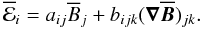 (A.1)Here aij and bijk are tensors determined by the fluid flow. The gradient tensor
  can be split into an antisymmetric part, which can be expressed by , and a symmetric part
  . Therefore we may also write
 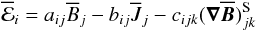 (A.2)with new tensors bij and cijk, the latter being symmetric in j and k. From the further assumption that the flow constitutes an axisymmetric turbulence we may conclude that aij, bij and cijjk are axisymmetric tensors. Defining the preferred direction by the unit vector we then have
 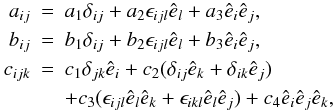 (A.3)with coefficients a1, a2, ..., c4 determined by the fluid flow. Taking (A.2) and (A.3) together and considering that
 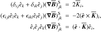 (A.4)we find
 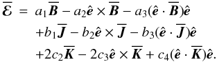 (A.5)Since
  there is no contribution with c1. With a proper renaming of the coefficients (A.5) turns into (3).
All Tables
Dependence of the density contrast ρbot/ρtop and the degree of anisotropy , for three different values of kf/k1, on the density stratification for nonrotating turbulence.
All Figures
|
Fig. 1 The coefficients |
| In the text | |
|
Fig. 2 Co dependence of transport coefficients in a model with rotation but zero density stratification, Rm ≈ 9, Pm = Sc = 1, Gr = 0, kf/k1 = 5. |
| In the text | |
|
Fig. 3 Anisotropy |
| In the text | |
|
Fig. 4 Gr dependence of the transport coefficients in a model with density stratification but zero rotation, Pm = Sc = 1, Rm ≈ 22, Co = 0, kf/k1 = 5. |
| In the text | |
|
Fig. 5 Co dependence of transport coefficients in a model with rotation and density stratification, Pm = Sc = 1, Rm ≈ 10, Gr ≈ 0.16, kf/k1 = 5. |
| In the text | |
|
Fig. 6 k∥ dependence of transport coefficients in a model with rotation and density stratification, |
| In the text | |
|
Fig. 7 Same as Fig. 6, but k⊥ dependence, k∥ = k1. The filled and open circles denote results for α⊥, β⊥, κ⊥, and |
| In the text | |
|
Fig. 8 Dependencies of the transport coefficients on Rm or Pe in a model with rotation and density stratification, Pm = Sc = 1, Co = 1.0, Gr = 0.16, kf/k1 = 5. |
| In the text | |
Current usage metrics show cumulative count of Article Views (full-text article views including HTML views, PDF and ePub downloads, according to the available data) and Abstracts Views on Vision4Press platform.
Data correspond to usage on the plateform after 2015. The current usage metrics is available 48-96 hours after online publication and is updated daily on week days.
Initial download of the metrics may take a while.