| Issue |
A&A
Volume 545, September 2012
|
|
|---|---|---|
| Article Number | A151 | |
| Number of page(s) | 32 | |
| Section | Astronomical instrumentation | |
| DOI | https://doi.org/10.1051/0004-6361/201219614 | |
| Published online | 24 September 2012 | |
Instantaneous phase retrieval with the vector vortex coronagraph
Theoretical and optical implementation
1 60 rue des bergers, 75015 Paris, France
e-mail: This email address is being protected from spambots. You need JavaScript enabled to view it.
2 Université de Liège, 17 Allée du 6 Août, 4000 Sart Tilman, Belgium
3 European Southern Observatory, Alonso de Cordóva 3107, Vitacura, Santiago, Chile
e-mail: This email address is being protected from spambots. You need JavaScript enabled to view it.
4 NASA-Jet Propulsion Laboratory, California Institute of Technology, 4800 Oak Grove Drive, Pasadena, CA 91109, USA
5 Techspace-Aero, route de Liers 121, 4041 Milmort, Belgium
e-mail: This email address is being protected from spambots. You need JavaScript enabled to view it.
Received: 16 May 2012
Accepted: 19 July 2012
Abstract
Coronagraphs are used as high-contrast imaging tools. However, it is well-known that the achievable contrast is primarily limited by wavefront aberrations in the optical train. Various kinds of devices and methods have been proposed to correct and calibrate these errors and, hence, improve the efficiency of coronagraphs. Here, we present an innovative idea that allows instantaneous measuring of the phase and the amplitude of residual stellar speckles in coronagraphic images. The technique is based on the unique polarization properties of the vector vortex coronagraph, which serves as a new type of phase diversity (POAM diversity), as well an extension of the Nijboer-Zernike theory of aberrations. We also propose and discuss a simple practical optical implementation of the technique, which only requires polarization splitting at the back-end of any existing vector vortex coronagraph systems.
Key words: instrumentation: high angular resolution / instrumentation: adaptive optics / methods: numerical / techniques: polarimetric
© ESO, 2012
1. Introduction
The direct detection of exoplanets is limited by both the contrast and the angular separation between the planet and its host star. For example, in the visible, Earth-like exoplanets would be 1010 times fainter than their host stars and located within a fraction of an arcsecond even for nearby systems. Many coronagraphs have been proposed to suppress the starlight diffracted light, but all of them are limited by the imperfections of the entrance wavefront: residual speckle patterns are the dominant source of noise in the high-contrast imaging. Even when using high-order or extreme adaptive optics (XAO), the performance of coronagraphs is still limited by the phase and the amplitude knowledge used for the dark-hole generation, and maintenance while acquiring science data (Bordé & Traub 2006; Give’on et al. 2007). We propose to measure the speckle phase and amplitude simultaneously with the science integration using the polarization properties of the vectorial vortex coronagraph (VVC), Mawet et al. (2005), Mawet et al. (2009). For that, we split the output pupil field into its two orthogonal circular polarization components with a simple circular polarization splitter (see Sect. 6). In this paper, we analytically demonstrate, using the polar Nijboer-Zernike diffraction theory of light (Magette 2010), that the polarized VVC coronagraphic images present sufficient diversity to retrieve the phase and the amplitude information of the wavefront at the telescope entrance pupil. The main advantage of the proposed optical implementation and phase retrieval scheme is its simplicity and quasi-instantaneous nature. It allows minimizing the non-common path wavefront errors in the optical system. It also presents a high transmission coefficient, higher than 90%.
The retrieved wavefront complex amplitude of the telescope pupil can be used directly as a synthetic reference image with image subtraction or as a dynamic speckles calibration system using adaptive optics corrections (amplitude and phase).
The paper is organized as follows: first, we briefly present the Nijboer-Zernike diffraction theory for low and high levels of aberrations in Sect. 2. The extension of the NZ theory for the vortex coronagraph is presented in Sect. 3, followed by a detailed presentation of the phase and amplitude retrieval procedure in Sect. 4. The overall system architecture adopted for our speckles calibration system is presented in Sect. 6. Finally, the phase retrieval accuracy under “end-to-end” numerical simulations is presented in Sect. 7.
2. The Nijboer-Zernike theory
The Nijboer-Zernike (NZ) theory emerged from the work of Nijboer (1943) on the diffraction theory of aberrations in polar coordinates. Nijboer first introduced the relation between the diffraction equation and the optical aberrations expressed in the form of Zernike polynomials. However, the complexity of the equations forced him to limit his theory to small aberrations, typically smaller than one wave (Nijboer 1947). Janssen (2002) later completed Nijboer’s theory by using an explicit Bessel series representation for the diffraction integral (high-order Hankel transforms). He also proposed a convenient way to numerically compute the expressions that involve these Bessel series (the  functions, discussed below). This extended NZ theory allows one to quickly and analytically compute the intensity point spread function (PSF) of any complex system with circular pupil from its known aberrations.
2.1. Fraunhofer diffraction integral of an aberrated pupil in polar coordinates
The expression of the complex amplitude in the image plane U(r,φ) as a function of the pupil complex amplitude P(ρ,θ) can be calculated by the well-known Fraunhofer diffraction integral, expressed here in polar coordinates: 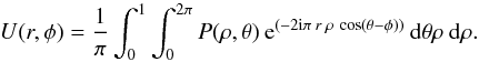 (1)The integration limits are defined by the pupil function 0 ≤ r ≤ 1 and 0 ≤ θ ≤ 2π. The pupil function itself can be expressed in terms of Zernike polynomials using classical Zernike coefficients α, or the generalized coefficients β, defined as follows (Magette 2010):
  (2)The Zernike polynomials
  are defined as usual:
 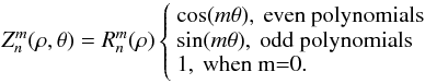 (3)where
  is a radial polynomial defined as
  (4)The radial polynomials
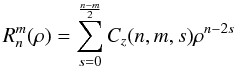
  are even or odd in ρ depending on the n,m values. Note that the polynomials corresponding to m = 0 are treated as even polynomials since cos(0) = 1. Wavefront surface development with Zernike polynomials, and the full expression of the Cz(n,m,s) coefficients is detailed in Appendix A.
2.2. General Zernike coefficients 
Under the small aberrations assumption, the simplified expression of the pupil aberrations  is generally sufficient to describe the entrance wavefront, and simply connects the
  and
and  coefficients by identification of the terms in Eqs. (2). The and coefficients capture both phase and amplitude aberrations.
The use of general Zernike coefficients  1 is preferable since they corresponds to the proper aberration basis of the NZ theory. However, the physical interpretation of the coefficients is not as easy as for the usual
  Zernike coefficients. Here, for the sake of completeness and accuracy, we chose to use the generalized Zernike coefficients . Subsequently, the Fraunhofer diffraction integral given in the Eq. (1) can be seen as a linear system:
  (5)
(5) is the image plane complex amplitude corresponding to the Zernike polynomial (n,m).
For the sake of simplicity, we split the coefficients into two categories:  for even Zernike polynomials (cos), and
  for odd Zernike polynomials (sin),
 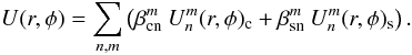 (6)Detailed analytical expressions of the
  complex amplitudes are given in Appendix C.
3. Extension of the NZ theory for the vector vortex coronagraph
3.1. The vector vortex voronagraph
The VVC is a transparent focal plane phase-mask that creates two opposite phase screw dislocations Exp![Mathematical equation: \hbox{$\left[\pm {\rm i} l_{\rm p} \phi\right]$}](/articles/aa/full_html/2012/09/aa19614-12/aa19614-12-eq35.png) , with lp the topological charge or the photon orbital angular momentum (POAM, Poynting 1909; Yao & Padgett 2011), and φ the azimuthal coordinate. When the phase singularity is centered on the PSF, it redirects the starlight outside the pupil where it can be blocked by a Lyot stop (Mawet et al. 2005).
, with lp the topological charge or the photon orbital angular momentum (POAM, Poynting 1909; Yao & Padgett 2011), and φ the azimuthal coordinate. When the phase singularity is centered on the PSF, it redirects the starlight outside the pupil where it can be blocked by a Lyot stop (Mawet et al. 2005).
3.2. Field expression at the coronagraph
The effect of a VVC with a topological charge lp on the complex amplitude of the PSF can be written as ![Mathematical equation: \begin{equation} \label{eq:amp_vort} U_v(r,\phi,l_{\rm p}) = {\rm exp}{\left[{\rm i} \left( l_{\rm p} \phi-\pi/2 \right)\right]} \cdot U(r,\phi), \end{equation}](/articles/aa/full_html/2012/09/aa19614-12/aa19614-12-eq38.png) (7)where lp = 2 and lp = −2 correspond to the right-handed and left-handed POAM in circular polarization vector basis, respectively.
(7)where lp = 2 and lp = −2 correspond to the right-handed and left-handed POAM in circular polarization vector basis, respectively.
Using the expression for U(r,φ) previously defined, the complex amplitude in the coronagraph image plane, Uv(r,φ,lp) becomes:  (8)The Cm(φ) and Sm(φ) functions are defined as
  r,φ are the polar coordinates in the the coronagraphic image plane, and lp, Sign(lp) are the VVC topological charge and the chirality of the modulation, respectively.
The  functions are defined for cosine and sinus modes as follows (see Appendices D and E):
  (12)The impact of the
  on the intensity distribution is to azimuthally modulate the residual aberrations. Note that the are normalized in intensity (see Appendix F). Let us now extract the dominant term (n = N, m = 0) from the sum and rewrite Eq. (7) as
  (13)where the ~ symbol means that the term (n = N, m = 0) is absent from the sum.
  is larger than the other . This separation allows us to virtually create a dominant linear term with respect to the optical aberrations. In other words, as we will see in the following section, the extraction from the sum yields the coupled modal functions
  , present in the linear term of the final intensity expression, which have the key property
  .
.
3.3. Expression of the coronagraphic intensity
The action of the VVC is to redirect the field amplitude outside of the relayed pupil, conjugate to the entrance pupil. The coronagraphic suppression of starlight is then obtained by inserting a diaphragm smaller than the pupil diameter into this pupil plane, called the “Lyot stop”. The coronagraphic intensity in the camera plane downstream from the Lyot stop plane is (see Appendix M) ![Mathematical equation: \begin{eqnarray} \label{Ic} I_{\rm c}(r,\phi,l_{\rm p}) &=& \left| U_v(r,\phi,l_{\rm p})\right|^2 \quad \rightarrow \quad I_{\rm c}(r,\phi,l_{\rm p}) \nonumber \\ &=&4\left( \beta_N^0(d_{\rm c})\right)^2 \cdot \left|V_{N,0}^{l_{\rm p}} \right|^2 +f^{(1)}\left[\beta_{\rm cn}^m(d_{\rm c}),\beta_{\rm sn}^m(d_{\rm c})\right] +f^{(2)}\left[(\beta_{\rm cn}^m(d_{\rm c}))^2,(\beta_{\rm sn}^m(d_{\rm c}))^2,(\beta_{\rm cn}^m(d_{\rm c})\cdot\beta_{\rm sn}^m(d_{\rm c}))\right]. \end{eqnarray}](/articles/aa/full_html/2012/09/aa19614-12/aa19614-12-eq57.png) (14)It is composed of three different terms:
(14)It is composed of three different terms:
-
-
![Mathematical equation: \hbox{$f^{(1)}\left[\beta_{\rm cn}^m(d_{\rm c}),\beta_{\rm sn}^m(d_{\rm c})\right]$}](/articles/aa/full_html/2012/09/aa19614-12/aa19614-12-eq59.png) : a linear function of inner products between the
: a linear function of inner products between the  coefficients and the
  term.
term. -
![Mathematical equation: \hbox{$f^{(2)}\left[(\beta_{\rm cn}^m(d_{\rm c}))^2,(\beta_{\rm sn}^m(d_{\rm c}))^2,(\beta_{\rm cn}^m(d_{\rm c})\cdot\beta_{\rm sn}^m(d_{\rm c}))\right]$}](/articles/aa/full_html/2012/09/aa19614-12/aa19614-12-eq62.png) : a term quadratic in the coefficients and cos/sin cross terms.
: a term quadratic in the coefficients and cos/sin cross terms.
Note that in practice, the Lyot stop is always slightly undersized compared to the pupil, which in the present NZ theory simply yields a normalization of the radial Zernike polynomials with the diaphragm size dc < 1. The general coefficients then become a function of (dc):  (see Sect. 5.2).
4. NZ phase retrieval theory
The NZ phase retrieval method is based on the projection of the measured PSF on the basis of template modes, which leads to a system of decoupled linear equations. We first assume linearity: ![Mathematical equation: \begin{equation} \label{eq_approx} I_{\rm c}\approx 4\left( \beta_N^0(d_{\rm c})\right)^2 \cdot \left|V_{N,0}^{l_{\rm p}} \right|^2+f^{(1)}\left[\beta_{\rm cn}^m(d_{\rm c}),\beta_{\rm sn}^m(d_{\rm c})\right] \qquad f^{(2)}\left[(\beta_{\rm cn}^m(d_{\rm c}))^2,(\beta_{\rm sn}^m(d_{\rm c}))^2,(\beta_{\rm cn}^m(d_{\rm c})\cdot\beta_{\rm sn}^m(d_{\rm c}))\right]<f^{(1)}\left[\beta_{\rm cn}^m(d_{\rm c}),\beta_{\rm sn}^m(d_{\rm c})\right]. \end{equation}](/articles/aa/full_html/2012/09/aa19614-12/aa19614-12-eq66.png) (15)However, note that the quadratic term will be accounted for later on by a recursive corrector approach (see Sect. 4.3).
(15)However, note that the quadratic term will be accounted for later on by a recursive corrector approach (see Sect. 4.3).
In practice, its implementation is a two-step process. On one hand, it requires projecting the measured PSF on the basis of radial template modes by means of a polar Fourier transform: 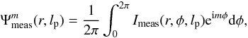 (16)where Imeas(r,φ,lp) is the measured coronagraphic image, which depends on lp, the topological charge.
On the other hand, the same projection is performed analytically on the final intensity expression Eq. (14):  (17)where Ic(r,φ,lp) is the analytical expression of the final coronagraphic image for the topological charge lp.
Comparing both the measured PSF decomposition and the analytically modeled one leads to the formation of decoupled systems of linear equations.
4.1. Modal analysis of the analytical intensity equation
The analytical expression of the linear term f(1) of the coronagraphic intensity is ![Mathematical equation: \begin{eqnarray} \label{flvr} f^{(1)}\left[\beta_{\rm cn}^m(d_{\rm c}),\beta_{\rm sn}^m(d_{\rm c})\right]= && \sum_{n,m}^{\sim}\left[A_{\rm c}^m\cdot 8\Re\left({\rm i}^m V_{n,m}^{l_{\rm p}} \: V_{N,0}^{l_{\rm p}*}\right)\cdot C_m(\phi)\right] - \sum_{n,m}^{\sim}\left[B_{\rm c}^m\cdot 8\Im\left({\rm i}^m V_{n,m}^{l_{\rm p}} \: V_{N,0}^{l_{\rm p}*}\right)\cdot C_m(\phi)\right] \nonumber\\ &&+\, \sum_{n,m}^{\sim}\left[A_{\rm s}^m\cdot 8\Re\left({\rm i}^m V_{n,m}^{l_{\rm p}} \: V_{N,0}^{l_{\rm p}*}\right)\cdot S_m(\phi)\right] - \sum_{n,m}^{\sim}\left[B_{\rm s}^m\cdot 8\Im\left({\rm i}^m V_{n,m}^{l_{\rm p}} \: V_{N,0}^{l_{\rm p}*}\right)\cdot S_m(\phi)\right] \end{eqnarray}](/articles/aa/full_html/2012/09/aa19614-12/aa19614-12-eq72.png) (18)
(18)![Mathematical equation: \begin{eqnarray} \label{flvrb} &&A_{\rm c}^m=\Re(\beta_N^0(d_{\rm c}))\Re(\beta_{\rm cn}^m(d_{\rm c}))+\Im(\beta_N^0(d_{\rm c}))\Im(\beta_{\rm cn}^m(d_{\rm c})) \qquad A_{\rm s}^m=\Re(\beta_N^0(d_{\rm c}))\Re(\beta_{\rm sn}^m(d_{\rm c}))+\Im(\beta_N^0(d_{\rm c}))\Im(\beta_{\rm sn}^m(d_{\rm c})) \\[2mm] && B_{\rm c}^m=\Re(\beta_N^0(d_{\rm c}))\Im(\beta_{\rm cn}^m(d_{\rm c}))-\Im(\beta_N^0(d_{\rm c}))\Re(\beta_{\rm cn}^m(d_{\rm c})) \qquad B_{\rm s}^m=\Re(\beta_N^0(d_{\rm c}))\Im(\beta_{\rm sn}^m(d_{\rm c}))-\Im(\beta_N^0(d_{\rm c}))\Re(\beta_{\rm sn}^m(d_{\rm c})).~~~~~~~~~~~~~~ \end{eqnarray}](/articles/aa/full_html/2012/09/aa19614-12/aa19614-12-eq73.png) ℜ and ℑ are the real and imaginary parts, respectively. The complete demonstration is detailed in Appendix M.
ℜ and ℑ are the real and imaginary parts, respectively. The complete demonstration is detailed in Appendix M.
To facilitate the analytical computation of Eq. (17) using Eq. (18), we introduce the following functions: ![Mathematical equation: \begin{equation} \label{innerprod} \Psi_{n,m}^{l_{\rm p}}=-8 \epsilon_{m}^{-1}\Im\left[{\rm i}^m V_{n,m}^{l_{\rm p}} . V_{N,0}^{l_{\rm p}*}\right] \qquad \chi_{n,m}^{l_{\rm p}}=8 \epsilon_{m}^{-1}\Re\left[{\rm i}^m V_{n,m}^{l_{\rm p}} . V_{N,0}^{l_{\rm p}*}\right]. \end{equation}](/articles/aa/full_html/2012/09/aa19614-12/aa19614-12-eq76.png) (21)The Ψ and χ functions correspond to the phase and to the amplitude aberration templates, respectively. The full analytical computation presented in Appendix N demonstrates that the measured intensity
(21)The Ψ and χ functions correspond to the phase and to the amplitude aberration templates, respectively. The full analytical computation presented in Appendix N demonstrates that the measured intensity  in the polar Fourier plane is a linear combination of the phase and amplitude aberration templates
  and
and  .
.
We now multiply this result with and , which produces the “inner” products of the aberration templates, physically corresponding to the autocorrelation between the phase and amplitude aberration templates: 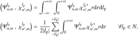 (22)It can easily be demonstrated that these inner products have the following properties:
 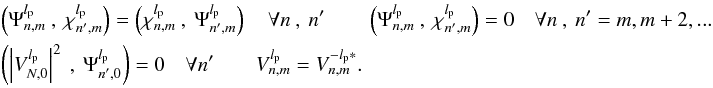 (23)Using the inner products, it is now possible to build a linear system of equations,
 ![Mathematical equation: \begin{eqnarray} \label{lse1} && G_{n,n'}^{m,l_{\rm p}}\left(\Psi\right).u\left[\beta_n^m \right]=r_{n'}^{m,l_{\rm p}}\left(\Psi\right) \qquad G_{n,n'}^{m,l_{\rm p}}\left(\chi\right).u\left[\beta_n^m \right]=r_{n'}^{m,l_{\rm p}}\left(\chi\right) \\ && G_{n,n'}^{m,l_{\rm p}} \left(\Psi\right) = \left(\Psi_{n,m}^{l_{\rm p}}\:,\:\Psi_{n',m}^{l_{\rm p}}\right) \qquad G_{n,n'}^{m,l_{\rm p}} \left(\chi\right) = \left(\chi_{n,m}^{l_{\rm p}}\:,\:\chi_{n',m}^{l_{\rm p}}\right) \qquad r_{n'}^{m,l_{\rm p}}\left(\Psi\right) = \left(\Psi_{\rm meas}^{m}\:,\:\Psi_{n',m}^{l_{\rm p}}\right) \qquad r_{n'}^{m,l_{\rm p}}\left(\chi\right) = \left(\Psi_{\rm meas}^{m}\:,\:\chi_{n',m}^{l_{\rm p}}\right) \nonumber \end{eqnarray}](/articles/aa/full_html/2012/09/aa19614-12/aa19614-12-eq84.png) (24)where G is a Gram matrix, and is defined with all possible inner products coefficients.
(24)where G is a Gram matrix, and is defined with all possible inner products coefficients. ![Mathematical equation: \hbox{$u\left[\beta_n^m \right]$}](/articles/aa/full_html/2012/09/aa19614-12/aa19614-12-eq85.png) is the vector containing the unknown coefficients , and r is a vector with the polar Fourier transform image analysis coefficients. Note that after the proper integration of the inner products the G matrix includes all three Pancharatnam topological charges − lp,0, + lp.
is the vector containing the unknown coefficients , and r is a vector with the polar Fourier transform image analysis coefficients. Note that after the proper integration of the inner products the G matrix includes all three Pancharatnam topological charges − lp,0, + lp.
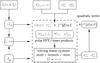 |
Fig. 1 Schematic view of the NZ vortex phase-retrieval process. It consists of using the real input coronagraphic images, corresponding to lp = 0, ± 2 (the lp = ± 2 images are provided by polarization splitting, while the unpolarized image (lp = 0) is directly given by the sum of the two polarized images) projected on aberrations templates, and finding the unknown coefficients by resolving a system of linear equations. Left: the three images needed for the full aberration analysis. Center: linear systems to retrieve the |
The r vector must be defined for three different cases: radial modes (m = 0), purely cosine modes, and purely sine modes. For radial modes, we use the cosine description. The end of Appendix N details the analytical expressions for all coefficients used in the matrix G and the two vectors u and r.
4.2. The f(1) term retrieval: solving a linear system of equations
Introducting the inner product (see Eq. (21)) allows us to calculate the linear term of the intensity equations (see Eq. (18)). The vectorial vortex complex amplitude retrieval is sensitive to the amplitude and the phase effects in the image. In practice, and to accelerate the convergence of the algorithm, we must bind the real part of the parameters (amplitude effect) to the most probable range of values. Indeed, amplitude and phase effects in the final intensity images are completely indistinguishable and potentially, many solutions exist. However, if we restrict ( ) to a physical solution, which corresponds to small amplitude errors, the algorithm converges quickly.
4.2.1. The  (dc) coefficient
The first term  (piston) is equal to zero in the ideal case (Mawet et al. 2005). For a single-dish telescope, the piston phase is a gauge invariant and we chose 0 for both the imaginary parts of
  and ,
and , 
 , the defocus term, is generally small, and can be easily minimized in practice. The first dominant purely radial mode is thus the spherical aberration (
 ). The first set of unknown coefficients to retrieve, , corresponds to the main aberration. When the images are projected onto the radial mode template basis , all coefficients will be compared to this term. As we developed in Eqs. (8), the Cm(φ) and Sm(φ) functions show a great variability for different m modes. Each case must then be processed separately (see the NZ retrieval diagram in Fig. 1).
4.2.2. Resolution of the system for m = 0
If m = 0, the vector of unknown coefficients u can be written as ![Mathematical equation: \begin{equation} \label{lse2} u_1=\left[\left(\beta_N^0 \right)/2, A_{\rm c}^0(0),...,A_{\rm c}^0(n_{\rm max})\right]\qquad u_2=\left[B_{\rm c}^0(0),...,B_{\rm c}^0(n_{\rm max})\right], \end{equation}](/articles/aa/full_html/2012/09/aa19614-12/aa19614-12-eq104.png) (25)where nmax is the maximum number of modes. The first system (u1) allows determining the coefficient. Previously, we fixed the piston term
(25)where nmax is the maximum number of modes. The first system (u1) allows determining the coefficient. Previously, we fixed the piston term  but in the practical real-life case (Fresnel diffraction and finite coronagraphic mask), this coefficient is not zero. This piston term corresponds to the mask limitation in the considered optical system (chromaticity, F-number, small Lyot dot in the center, Lyot stop in the pupil plane, etc.) and must be calibrated on the optical system before astronomical use. In that case, the complex value of the coefficient can be fixed in the diffraction model and the coefficient required for the retrieval is known thanks to the resolution of the first equation with
  ,
,  and
and  .
.
4.2.3. Resolution of the system for 0 < m < n
If 0 < m < n, the vector of unknown coefficients u given by Eq. (24) can be written as ![Mathematical equation: \begin{equation} \label{lse2bis} u_1=\left[A^m_{\rm c}(0),...,A^m_{\rm c}(n_{\rm max})\right]\qquad u_2=\left[B^m_{\rm c}(0),...,B^m_{\rm c}(n_{\rm max})\right]\qquad u_3=\left[A^m_{\rm s}(0),...,A^m_{\rm s}(n_{\rm max})\right]\qquad u_4=\left[B^m_{\rm s}(0),...,B^m_{\rm s}(n_{\rm max})\right]. \end{equation}](/articles/aa/full_html/2012/09/aa19614-12/aa19614-12-eq113.png) (26)
(26)
4.2.4. Resolution of the system for m = n
In the case where m = n, the vector of unknown coefficients u has to be calculated separately, and the vector can be written as: ![Mathematical equation: \begin{eqnarray} \label{lse3} &&u_1=\left[A^n_{\rm c}(0)+A^n_{\rm s}(0),...,A^n_{\rm c}(n_{\rm max})+A^n_{\rm s}(n_{\rm max})\right]\qquad u_2=\left[B^n_{\rm c}(0)+B^n_{\rm s}(0),...,B^n_{\rm c}(n_{\rm max})+B^n_{\rm s}(n_{\rm max})\right]\\ &&u_3=\left[A^n_{\rm c}(0)-A^n_{\rm s}(0),...,A^n_{\rm c}(n_{\rm max})-A^n_{\rm s}(n_{\rm max})\right]\qquad u_4=\left[B^n_{\rm c}(0)-B^n_{\rm s}(0),...,B^n_{\rm c}(n_{\rm max})-B^n_{\rm s}(n_{\rm max})\right].\nonumber \end{eqnarray}](/articles/aa/full_html/2012/09/aa19614-12/aa19614-12-eq116.png) (27)The complete demonstrations for the
(27)The complete demonstrations for the  coefficients are detailed in Appendix N.
4.3. The quadratic correction f(2): the predictor-corrector approach
Keeping only the linear term of the final coronagraphic intensity allows us to simplify the retrieval process using linear algebra only. This approximation allows determining the coefficients with a precision of a few percents. However, in a coronagraphic system, coupling between phase and amplitude appears due to the crossed terms in “sin / cos”. These terms are also quadratic and are taken into account in the predictor-corrector analysis.
In this section, we introduce an improvement that allows us to account for the quadratic terms. When a coronagraphic device is used,  is attenuated and the purely quadratic phase terms and the amplitude-phase coupled terms are of the same order of magnitude. They should thus be taken into account. Hereafter, we present a simple way of doing this using a predictor-corrector approach. This technique proceeds as follows:
 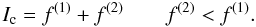 (28)The retrieval approach presented previously is based on the following simplification: Ic ≈ f(1).
Solving this equation leads to a first approximation  of , which corresponds to an image
  such that
  .
.
 is then defined based on approximating the exact quadratic term.
After several iterations, tends to if, and only if, f(2) < f(1).
The predictor-corrector approach as in the classical NZ phase retrieval (Magette 2010) leads to a better estimation of the coefficients.
4.4. Phase amplification
An optical vortex phase-mask “amplifies” the small input pupil phase error ( ) on the output coronagraphic pupil. As already suggested in Sect. 4, the first term
  . This is why in the coronagraphic image plane all wavefront errors in the entrance pupil plane are enhanced by the phase-mask coronagraphic device. Indeed, in the proposed phase-retrieval analysis, we compare all Zernike polynomials with the first non-zero term in the linear system equations to avoid numerical singularities. A good estimation of the term remains mandatory to allow a correct wavefront retrieval.
4.5. The  coefficient
The coefficient remains a free variable, and it is naturally obtained with the value of the nulling factor.
Indeed, the nulling coefficient ϵc can be defined as the sum of all residual aberrations in the coronagraphic pupil plane, 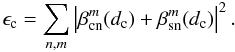 (29)We calibrate the nulling factor with an instrumental PSF of the optical system without any coronagraphic device (the lp = 0 term). In our NZ development, the sum of the two circular polarization images can be used as lp = 0 image. This composite image can be seen as the instrumental PSF from which the perfect Airy pattern |J1(r)/r|2 has been subtracted.
4.6. Optimum number of images for phase retrieval
In the classical phase diversity algorithm (Gonsalves 1982; Blanc et al. 2003), the estimation of the entrance aberrations from the sole focused image does not ensure the uniqueness of the solution. Indeed, two different aberrations can produce the same PSF in the image plane. At least, two images with known phase variations are needed to remove this indetermination. If the phase diversity is performed in the pupil plane as in Roddier & Roddier (1993), the result is the same: two images of defocused pupil are needed. The indetermination is fully removed if the two images are π phase-shifted. This is the case of phase retrieval using classical NZ theory (with focus variation ± f), and in this modified NZ theory for the VVC device (with POAM modulation ± lp).
In coronagraphy, another indetermination appears: the residual speckle pattern changes in intensity with the entrance Strehl ratio due to the induced variation of the coronagraph rejection factor, but not in overall morphology. Therefore, the absolute values of need to be retrieved using a good estimation of , (see the previous section). For that, a third image, such as a simple PSF is the key to ensure a true phase retrieval. Moreover, for space telescopes, the PSF allows taking “telescope breathing” (equivalent to Strehl variations) effects into account.
5. Phase retrieval in the presence of practical limitations
In addition to phase and amplitude wavefront errors, starlight suppression is also limited by intrinsic properties of the optical system and features of the coronagraphic device: for instance, the telescope central obscuration (see Appendix H.2) and support structures (see Appendix L). In the following, we review the impact of these characteristics on the phase retrieval process.
5.1. Annular pupil
For an on-axis telescope with a central obscuration ϵ (ϵ < 1), the full aberration retrieval can be obtained directly by replacing the Cz(n,m,s) Zernike coefficients (see Eq. (4)) with the Cz(n,m,s,ϵ) using the normalization described in Mahajan (1981a,b),  (30)Even though the complex amplitude pupil retrieval process presented in this paper is fully applicable (see Appendix B) to on-axis telescopes, for the sake of simplicity, the ϵ coefficient is omitted.
5.2. Impact of the Lyot stop diameter
The main effect of the diaphragm dc (Lyot stop) in the coronagraphic pupil plane (Lyot plane) is to reduce the coherent term of the diffraction by a factor ϵc. The second effect of the Lyot stop is to rescale the Zernike radial polynomial as 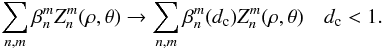 (31)We derived a recurrence formula to calculate the in Appendix I, yielding, with n = m,m + 2,...:
 ![Mathematical equation: \begin{equation} \label{new_orth_finside} \beta_n^m(d_{\rm c})=\sum_{n'} \beta_{n'}^m \cdot \left[ R_{n'}^n(d_{\rm c})-R_{n'}^{n+2}(d_{\rm c}) \right] \qquad \beta_n^m= (n+1) \sum_{n'} \beta_{n'}^m(d_{\rm c}) \cdot \frac{\left[ R_{n}^{n'}(d_{\rm c})-R_{n}^{n'+2}(d_{\rm c}) \right]} {(n'+1)}, \nonumber \end{equation}](/articles/aa/full_html/2012/09/aa19614-12/aa19614-12-eq143.png) where
where  and
and  . The coefficients are simply normalized to the size of the diaphragm in the Lyot plane.
5.3. Lyot stop optimization
The Lyot plane field expression is presented in Appendix D under the assumption of Fraunhofer diffraction, and in Appendix H under the Fresnel propagation assumption, respectively. The Fresnel number  is generally larger than 100, where dc is the radius of the Lyot stop and z is the propagation distance. The Fresnel case thus only shows a slight blurring effect of the pseudo-Zernikes polynomials given in the Fraunhofer approximation. Therefore, the Fraunhofer diffraction is sufficient to describe coronagraphic aberration residuals in the pupil plane. As far as the pupil edge effect is concerned, the Lyot stop has to cover enough residual rings inside the pupil plane to ensure a proper nulling ratio (see Appendix K).
5.4. The imperfect vortex device
The VVC manufacturing imperfections lead to the following error terms:
-
The phase-shift error with respect to π (chromaticity).
-
The region in the center of the mask may present a deviation from the overall large-scale pattern called the region of disorientation (this defect largely depends on the technological approach chosen to manufacture the vortex device).
-
The finite size of the mask in the coronagraphic image plane.
These terms can be taken into account in the coronagraphic NZ retrieval by a simple Fourier simulation to estimate the  term (see Appendices J and L for more details).
6. Practical implementation
In this section, we present the instrumental concept we propose to instantaneously acquire the phase-amplitude information about the residual wavefront errors. We propose to use a simple Wollaston device coupled to a pair of achromatic quarter-wave plates to separate the coronagraphic images into left and right circular polarizations, allowing for a simple optical implementation that minimizes non-common path errors. Figure 2 illustrates the optical implementation downstream of the Lyot stop.
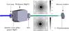 |
Fig. 2 Polarization splitter analysis: possible implementation of the polarization splitter system used after the Lyot stop. An achromatic quarter-wave plate (quartz/MgF2) and a Wollaston in MgF2 combined here with a simple achromatic doublet. This simple optical implementation allows us to image the two residual coronagraphic images in the left and right circular polarization basis on the detector. The two images presented in this figure in logarithmic gray scale show the two polychromatic PSF (650–900 nm) obtained by this simple scheme for the two circular polarization images. Note that the PSF shows a small chromatic smearing residual on the x-axis (Strehl = 96.5%) due to the substantial wavelength bandpass. This polychromatic smearing is detailed in Appendix P. |
6.1. Tolerancing of the optical design
To show the validity of our approach, we considered potential sources of disturbances one by one. First of all, the entrance pupil introduces its own time-evolving phase defects due to polishing errors and time-dependent thermal effects. The latter affect low-order Zernikes and will be simulated with a power spectral density (PSD) of f-2. The coronagraphic device possesses its own limitation (manufacturing defect and chromatism, see Sect. 5.4), which need to be taken into account as well.
Thick optical devices such as quarter-wave plates, Wollaston and the lens/mirrors are the sources of four types of second-order aberrations:
-
Polishing errors: represented by a PSD with wavefront error (WFE) < λ/50 rms for low spatial frequencies, and < 0.2 nm rms in the roughness scale (see optical specifications in Riaud et al. 2003).
-
Non-common path aberration: due to the small beam separation angle, it is expected that only roughness will play a significant role; we chose to represent it with two phase screens of 0.2 nm rms each.
-
Light scattering in thick materials, ghost features: scattering limitation and ghost features of the proposed calibration analysis system are calculated directly with the scattering function (see the Appendix O) and the Zemax software.
-
Residual polarization ellipticity due to non-ideal retardation over the entire wavelength range: the quarter-wave plates were optimized Riaud (2003), and we obtained a plate thickness of 0.24104 mm and 0.30792 mm at 20°C for the MgF2 and the quartz material, respectively. These thicknesses must be controlled to 1 μm with a Babinet compensator and the plate temperature must be controlled to ±0.5°C. The residual phase error becomes σ2 = 0.021 radian for the entire spectral bandpass.
The numerical simulations show that the scattering in the glass material is about 10-6−10-7 of the entrance residual coronagraphic starlight, which is not a problem even for Earth-like planet detection provided that the first coronagraphic stage is efficient enough to remove most of the starlight (ϵc < 10-4).
7. End-to-end modeling
This section presents thorough numerical simulations. The goal of these simulations is to show that the entrance pupil wavefront phase can be retrieved even in the presence of real-life optical imperfections, and to which level of accuracy it can be retrieved. Usually, we model a coronagraphic instrument using FFT-based optical propagation; three FFT are needed to fully simulate a coronagraphic image. Here, we used our NZ modal decomposition of the entrance aberrations seen through the VVC to directly construct the final image. Before going into the details of the end-to-end modeling, we tested our analytical method vs. a FFT-based propagation prescription to show their equivalence.
7.1. Analytical vs. Fourier propagation
To study the accuracy of the modal decomposition with the analytical functions, we performed numerical simulations with FFT and the direct expression of modal functions. The entrance pupil is a perfect unobscured circular pupil affected by wavefront (polishing) errors described by a set of Zernikes up to n = 860 with a weighting of 1/(n + 1)2, leading to an initial Strehl ratio of 95%. Note that the FFTs must be performed with large arrays (2K × 2K) or (4K × 4K) to minimize aliasing effects. Super-sampling is also used in the coronagraphic plane. All simulations are preformed for the following two cases: the βn,m representation in the pupil plane ( ) and the αn,m classical representation (
 ). The Nijboer-Zernike uses the first pupil representation and is not limited to high Strehl ratio (see Appendix A for a full analysis). Figure 3 compares the analytical NZ functions under the two pupil representations. Note that FFT simulations always show a high-frequency residual noise. Moreover, the FFT propagation through the VVC acts as a high-pass filter, artificially minimizing the residual coronagraphic stellar flux in the final image near the center. The NZ analytical functions do not present these problems: they are very fast and more accurate. For a complete comparison between the semi-analytical and pure numerical method, see Appendix G.
7.2. Summary of simulation parameters
We present realistic polychromatic simulations incorporating the various defects detailed above.
-
Using the first 860 Zernikes (40 complete modes), the input Strehl ratio is set to 95% @ 650 nm.
-
An imperfect phase-mask: where the s-transmittance is 97%, the p-transmittance is 98% and the local phase retardance is π ± Δφ, while following a quadratic law (see Eq. (P.1) in Appendix P.2).
-
The quarter-wave plates have an absolute phase dependence equal to (λ in μm): φqλ = 0.3442 + 2.94887λ − 1.74126λ2.
-
Common and non-common path errors are λ/71 rms @ 650 nm both (the total is λ/50 rms at 650 nm).
-
Polishing error: DSP f-2 and non-common path error.
-
Polychromatic speckle smearing due to residual Wollaston chromatism given by the Zemax model.
-
Photon noise, readout noise (6 e−), full-well capacity of 105e−, residual flat of 1% rms.
These inputs are commented on in Appendix P, where we also present the full sets of images.
 |
Fig. 3 Numerical simulation illustrating the principle of Nijboer-Zernike retrieval applied on the vortex coronagraph. (Up to down), numerical simulation for each circular polarization with lp = 2 and lp = −2 respectively using the first 860 Zernike polynomials (40 complete modes) and a Lyot stop of 99%. The Strehl ratio of the PSF before coronagraphic filtering is 95%. The Lyot stop remove the strong diffraction value in ρ = 1 but allows us to show all images without scaling the |


7.3. The accuracy functions
To quantify the quality of the proposed modal decomposition based on the NZ theory, we define the following  function:
  (32)This metric is applicable for all cases (monochromatic and polychromatic). But for a proper knowledge of the modal decomposition quality under adaptive optics correction (Krist et al. 2011), we can define the Err(σA) function
  (33)This function is applicable if we know the amplitude function
  of the coronagraphic residual. Indeed, this metric is only applicable in the monochromatic case. Numerical simulations for all Zernike modes for the monochromatic case are performed in Appendix G. This procedure allows us to estimate the robustness of our method in the two metrics. Table 1 presents the numerical accuracy of the NZ theory in the two presented metrics.
7.3.1. Polychromatic numerical simulations
Phase-mask coronagraphs are inherently chromatic, and so is the pure physical propagation process (see Fig. 4). The NZ phase retrieval must take that effect into account. A full set of simulated images is shown in Appendix P. We scanned all physical parameters (spectral bandpass and phase-shift error of the mask), including photon and detector noises below.
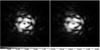 |
Fig. 4 Polychromatic coronagraphic simulation for lp = 2 with Δλ = 250 nm of spectral bandpass and a phase error of Δφ = ± 0.001 radian for the vortex mask. We also include defects of our optical implementation. Left: without the speckle smearing. Right: with the Wollaston speckle smearing. The chromatic effect on the speckles is small in the two cases, the contrast remains high. The brightness scale is the same between the two images and is not linear. |
7.3.2. RESULTS without photon noise
Here we test the maximum likelihood ( minimization) of the VVC coronagraphic images with the sum of monochromatic modal functions (see Appendix M). The first set of simulations is given without photon and readout noises. This process allows us to determine the global NZ phase retrieval behavior with respect to the wavelength bandpass and the phase-shift error on the coronagraphic device. Owing to the larger bandpass, we tuned the sampling of the NZ images. Numerical simulations are presented in Fig. 5, which shows the value variation as a function of the wavelength bandpass and the maximum phase-shift error of the vortex phase-mask (10-1/10-2/10-3 radian).
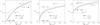 |
Fig. 5
|

We notice that simulations are presented for the two input basis  and
and  , but the second pupil phase decomposition is better suited for the NZ analysis. These simulations also show that the bandpass sets a limit of Err(σA) = 10-10 on the precision of the input electric field. The main result for our 95% of input Strehl ratio is that the NZ decomposition in the basis must be narrow band (Δλ = 65 nm or R = 10) to obtain the desired precision on the wavefront error. Now, with the photon limited image sets, we are only interested in the in:
  : modal decomposition.
7.3.3. RESULTS on photon-noise limited images
The previous simulations shows that the monochromatic modal decomposition is good with a small  for a Δλ < 100 − 150 nm. In this section, we present noisy simulations using the same monochromatic NZ modal functions to compare results with the previous ones. Figure 6 shows NZ retrieval results for coronagraphic images realistically limited by simulated detector (read-out,flat) and photon noises. A satisfying wavefront retrieval can be obtained after averaging at least 100 exposures. The gain for more exposures is only on the high order Zernike modes (n > 20).
To increase the precision of the retrieval with a broad bandwidth, we developed in Appendix E a polychromatic  set of functions. These functions take into account the contrast loss in the Bessel J rings due to the broad bandwidth. This effect would increase the robustness of the NZ retrieval. This new feature is added in the NZ algorithm.
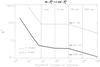 |
Fig. 6
|
8. Discussion
Thanks to the phase retrieval technique, we have shown in the previous sections that using POAM on the starlight given by the VVC, it is possible to instantaneously measure the phase of residual stellar speckles in coronagraphic images and hence improve the sensitivity of high-contrast telescopes. The main limitations are essentially coming from the limited coronagraphic nulling due to the input Strehl ratio, and the mask chromaticity over broad bandwidths. To investigate the impact of these instrumental limitations, we considered various input Strehl ratios in our simulations and estimated the coronagraphic nulling ratio and the maximum wavelength bandpass that are necessary to provide an accuracy as good as Err(σA) = 10-10. The results of this analysis are shown in Table 2. They were computed for an optimized high-contrast optical workbench for a best VVC (Δφ = 10-3 radian).
Maximum coronagraphic nulling ratio and wavelength bandpass achievable for various levels of input Strehl ratio.
Table 2 shows that our phase retrieval technique can still be used for a Strehl ratio as low as 95% with a mask chromaticity of 10-3 < Δφ < 10-2 radian provided that it is applied on a sufficiently narrow wavelength bandpass (65 nm). In practice, this means that the technique becomes more time-consuming because it must be applied on more spectral channels for decreasing Strehl ratios. Owing to the mask imperfection, a maximum nulling of 10-5 on the stellar peak seems to be feasible for an input Strehl ratio of 99.6%. The proposed method can handle various instrumental limitations and is sufficiently flexible to be coupled with the EFC algorithm (Give’on et al. 2007) to minimize the electric field in a desired region of the focal plane.
To ensure optimized wavefront corrections in the entrance pupil if we use an EFC algorithm, we need to use the complete Zernike development in the basis. We can null all present residual speckles in the the final coronagraphic image, not an individual speckle or identifiable feature only. Indeed, our process directly gives the input pupil phase and amplitude by image analysis but this is not an EFC algorithm. On the other hand, we must modify the EFC algorithm with our formalism to increase speed-up and obtain a direct global electric field minimization problem on the entrance pupil plane. A previous paper (Riaud 2012) on a new deformable mirror architecture provides all mathematical tools to use this NZ theory in the speckle cancellation process. Finally, we notice that if the corrections are not exactly in the pupil plane, some Fresnel propagations occur and small corrections of the Fraunhofer diffraction are needed (see Appendix H for a complete mathematical demonstration).
9. Conclusion
We demonstrated a full analytical modal decomposition of the effect aberrations on the vectorial vortex phase-mask final image using polarization properties. This procedure can be used on a very stable coronagraphic system for detecting terrestrial planets in the visible around nearby stars such as TPF-C (and precursors). Indeed, this proposed simple optical implementation allows us to calibrate the residual speckle pattern directly on the final coronagraphic images. End-to-end simulations show that the common and non-common path errors (λ/50 rms at 650 nm) after the filtered pupil due to the beam separation system are not influencing the final images. Indeed, the level of precision can be as good as ≈0.1% for the retrieved phase and is only limited by the detector and the photon noises. We also presented the effect of the polychromatic coronagraphic images on the maximum likelihood between the Fourier and the modal simulations. A precise ( ≈ 1%) modal decomposition with a wavelength bandpass of Δλ < 140 nm can be obtained with the proposed optical implementation. Finally, the main source of error and performance limitation of the presented modal decomposition is the signal-to-noise ratio of the two coronagraphic images and the direct PSF image (lp = 0). A very stable optical system is needed to stack several images ( ≈ 100 see Sect. 7.3.3) and reach the 10-10 speckle level that opens the way to detect terrestrial planets in the visible with a space telescope.
An option is the direct phase correction with extreme adaptive optics (XAO) to increase the rejection factor, the main limitation will again be the phase retrieval precision.
Details on the method for converting to for large aberrations (Strehl ratio > 50%) are given in Appendix A.
Acknowledgments
This work received the support of the University of Liège. This work was partly carried out at the European Southern Observatory (ESO) site of Vitacura (Santiago, Chile). The authors are grateful to C. Hanot (IAGL), D. Defrère (MPI-RA) for manuscript corrections. The authors wish to thank the referee Wesley Traub for his useful comments and corrections. The authors also acknowledge support from the Communauté française de Belgique – Actions de recherche concertées – Académie universitaire Wallonie-Europe. This idea dates back to 2005-2006 and the first author is grateful to section 17 and the CNAP French commissions for their outstanding recruitment work.
References
- Allen, L., Courtial, J., & Padgett, M. 1999, Phys. Rev. E, 60, 74977503 [CrossRef] [Google Scholar]
- Blanc, A., Fusco, T., Hartung, M., Mugnier, L. M., & Rousset, G. 2003, A&A, 399, 373 [NASA ADS] [CrossRef] [EDP Sciences] [Google Scholar]
- Bohren, C. F., & Huffman, D. R. 1983, Absorption and scattering of light by small particles (New York: Wiley) [Google Scholar]
- Bordé, P. J., & Traub, W. A. 2006, ApJ, 638, 488 [NASA ADS] [CrossRef] [Google Scholar]
- Born, M., & Wolf, E. 1999, Principles of Optics (Cambridge University Press) [Google Scholar]
- Give’on, A., Kern, B., Shaklan, S., Moody, D. C., & Pueyo, L. 2007, SPIE Conf. Ser., 6691, 66910A [Google Scholar]
- Gonsalves, R. A. 1982, Opt. Eng., 21, 829 [Google Scholar]
- Gradshteyn, I. S., & Ryzhik, I. M. 1994, Table of Integrals, Series and Products (Academic Press Inc), 1762 [Google Scholar]
- Henyey, L., & Greenstein, J. 1941, ApJ, 93, 70 [NASA ADS] [CrossRef] [Google Scholar]
- Janssen, A. 2002, JOSA A, 19, 849 [NASA ADS] [CrossRef] [Google Scholar]
- Krist, J. E., Belikov, R., Pueyo, L., et al. 2011, in SPIE Conf. Ser., 8151, 81510E [Google Scholar]
- Magette, A. 2010, Ph.D. Thesis: The International Liquid Mirror Telescope: optical testing and alignment using a Nijboer-Zernike aberration retrieval approch, IAGL, University of Liège, 1 [Google Scholar]
- Mahajan, V. N. 1981a, J. Opt. Soc. Am., 71, 75 [Google Scholar]
- Mahajan, V. N. 1981b, J. Opt. Soc. Am., 71, 1408 [Google Scholar]
- Mawet, D., Riaud, P., Absil, O., & Surdej, J. 2005, ApJ, 633, 1191 [NASA ADS] [CrossRef] [Google Scholar]
- Mawet, D., Serabyn, E., Liewer, K., et al. 2009, Opt. Expr., 17, 1902 [Google Scholar]
- ming Dai, G. 2006, J. Opt. Soc. Am. A, 23, 539 [NASA ADS] [CrossRef] [Google Scholar]
- Nijboer, B. 1943, Physica, 10, 679 [NASA ADS] [CrossRef] [Google Scholar]
- Nijboer, B. 1947, Physica, 13, 605 [NASA ADS] [CrossRef] [Google Scholar]
- Poynting, J. 1909, Proc. Roy. Soc. London Ser. A, 82, 560567 [NASA ADS] [Google Scholar]
- Riaud, P. 2003, Ph.D. Thesis, Université Paris VI [Google Scholar]
- Riaud, P. 2012, A&A, 545, A25 [NASA ADS] [CrossRef] [EDP Sciences] [Google Scholar]
- Riaud, P., & Schneider, J. 2007, A&A, 469, 355 [NASA ADS] [CrossRef] [EDP Sciences] [Google Scholar]
- Riaud, P., Boccaletti, A., Baudrand, J., & Rouan, D. 2003, PASP, 115, 712 [NASA ADS] [CrossRef] [Google Scholar]
- Roddier, C., & Roddier, F. 1993, J. Opt. Soc. Am. A, 10, 2277 [NASA ADS] [CrossRef] [Google Scholar]
- Yao, A. M., & Padgett, M. J. 2011, Adv. Opt. Photon., 3, 161 [CrossRef] [Google Scholar]
Appendix A: Expression of the pupil aberration function
A.1. Zernike decomposition of the wavefront
The general pupil function is 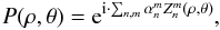 where
where  are the classical Zernike polynomials. When the aberration level is low (Strehl ratio > 90%), we can approximate this function by
  (A.1)The coefficients are then directly related to the classical coefficients. Since the Zernike polynomials form an orthogonal basis, the classical pupil function with can always be fully described by a sum of Zernike functions,
  (A.2)Note that the Strehl ratio Sr can be calculated directly with the coefficients:
  (A.3)By decomposing the real and imaginary parts of the pupil into Zernike polynomials, it is thus possible to obtain the real and imaginary parts of the β coefficients. If the coefficients represent the weights of the aberrations of the surface, the orthogonality relation yields
  (A.4)for the real and imaginary parts of Zernike polynomials.
High spatial frequency variations are difficult to represent with a limited sum of Zernike polynomials. More β coefficients than the number of α coefficients are then required to compute aberrations in the pupil. For coronagraphic imaging, where we use a diaphragm smaller than, or equal to, the pupil radius, the strong variations at the edge of the pupil are masked and the number of β and α coefficients are somewhat equal. The phase function φΠ(ρ,θ) of the pupil in the β basis can be determined by  (A.5)Because the arctangent function is defined between ± π, the phase function needs to be unwrapped before it is decomposed, if the level of aberrations is relatively high (Strehl < 80%).
A.2. Radial Zernike functions calculation
 (A.6)For a proper mathematical stability, the Cz(n,m,s) coefficients of the radial Zernike functions must be calculated recursively. The following radial Zernike functions can be calculated easily:
  (A.7)The low-order radial Zernike functions
  to
to  can be calculated with the following recurrence formula:
 ![Mathematical equation: \appendix \setcounter{section}{1} \begin{equation} \label{eq:zern_rad3} R_n^m(\rho)=\frac{n}{n^2-m^2}\left[\left( 4(n-1)\rho^2 -\frac{(n+m-2)^2}{n-2}-\frac{(n-m)^2}{n}\right)R_{n-2}^m(\rho) - \left( \frac{(n-2)^2-m^2}{n-2}\right)R_{n-4}^m(\rho)\right]. \end{equation}](/articles/aa/full_html/2012/09/aa19614-12/aa19614-12-eq248.png) (A.8)
(A.8)
Appendix B: Expression of the Hankel transform Hm
B.1. The classical Zernike radial functions 
To calculate the amplitude in the image plane in the presence of optical aberrations given by the Zernike polynomials, we need the direct mth order Hankel transform Hm for the radial coordinate. We have ![Mathematical equation: \appendix \setcounter{section}{2} \begin{eqnarray} \label{ht1} && H_m\left[R_n^m(\rho) \right]=\int_{0}^{1} \rho \, R_n^m(\rho) J_m(2 \pi r \rho) \: {\rm d} \rho\\ && \nonumber H_m\left[R_n^m(\rho) \right]=\sum^{\frac{n-m}{2}}_{s=0} C_z(n,m,s) \int_{0}^{1} \rho^{n-2s+1} J_m(2 \pi r \rho) \: {\rm d} \rho \quad \longrightarrow \quad \nonumber H_m\left[R_n^m(\rho) \right]=\sum^{\frac{n-m}{2}}_{s=0} f_z(n,m,s) . \end{eqnarray}](/articles/aa/full_html/2012/09/aa19614-12/aa19614-12-eq252.png) (B.1)The radial integration between the ρn − 2s + 1 polynomial and the Bessel function Jm can be calculated in the following way:
(B.1)The radial integration between the ρn − 2s + 1 polynomial and the Bessel function Jm can be calculated in the following way: ![Mathematical equation: \appendix \setcounter{section}{2} \begin{equation} \label{ht2} \int_{0}^{1} \rho^{n-2s+1} J_m(2 \pi r \rho) \: {\rm d} \rho = \frac{(\pi r)^m} {2} \frac{\Gamma\left[\frac{m+n}{2}-s+1\right]} {\Gamma\left[m+1\right] \cdot \Gamma\left[\frac{m+n}{2}-s+2\right]}\cdot {_2}F_1\left(\frac{m+n}{2}-s+1, m+1,\frac{m+n}{2}-s+2, -\pi^2 r^2\right) , \end{equation}](/articles/aa/full_html/2012/09/aa19614-12/aa19614-12-eq255.png) (B.2)where
(B.2)where  is the Gauss hypergeometric function. The full expression of the fz(n,m,s) function becomes
 ![Mathematical equation: \appendix \setcounter{section}{2} \begin{equation} \label{ht3} f_z(n,m,s)=\frac{(\pi r)^m (-1)^s \Gamma\left[n-s+1\right]} {2 \Gamma\left[m+1\right] \Gamma\left[s+1\right] \Gamma\left[\frac{n-m}{2}-s+1\right] \Gamma\left[\frac{n+m}{2}-s+2\right]} \cdot {_2}F_1\left(\frac{m+n}{2}-s+1, m+1,\frac{m+n}{2}-s+2, -\pi^2 r^2\right) . \end{equation}](/articles/aa/full_html/2012/09/aa19614-12/aa19614-12-eq258.png) (B.3)The Gauss hypergeometric function can be expressed in terms of Bessel J functions:
(B.3)The Gauss hypergeometric function can be expressed in terms of Bessel J functions: ![Mathematical equation: \appendix \setcounter{section}{2} \begin{equation} \label{ht4} \frac{J_{m+1}(2\pi r)}{2\pi r}=\frac{(\pi r)^m} {2 \cdot \Gamma\left[m+2\right]}\cdot {_2}F_1\left(m+1, m+1,m+2, -\pi^2 r^2\right) . \end{equation}](/articles/aa/full_html/2012/09/aa19614-12/aa19614-12-eq259.png) (B.4)After a simple variable change, the fz(n,m,s) function becomes
(B.4)After a simple variable change, the fz(n,m,s) function becomes ^{(n-m)/2}} { (\pi r)^x \Gamma\left[x+1\right] \Gamma\left[m+x+1\right] \Gamma\left[\frac{n-m}{2}-x+1\right]}\left( P(m) \frac{J_{m+x+1}(2\pi r)}{2\pi r} + Q(m) \frac{J_{m+x+2}(2\pi r)}{2\pi r}\right) , \end{eqnarray}](/articles/aa/full_html/2012/09/aa19614-12/aa19614-12-eq260.png) (B.5)where P(m) and Q(m) are two polynomials (see Table B.1). In fact, the summation of two fz functions (fz(n,m,x) + fz(n,m,x + 1)) allows us to simplify the general expression of the mth order Hankel transform. We use the following Bessel J transformation:
(B.5)where P(m) and Q(m) are two polynomials (see Table B.1). In fact, the summation of two fz functions (fz(n,m,x) + fz(n,m,x + 1)) allows us to simplify the general expression of the mth order Hankel transform. We use the following Bessel J transformation:  (B.6)After Bessel J functions simplification, we obtain
 ![Mathematical equation: \appendix \setcounter{section}{2} \begin{equation} \label{ht6} H_m\left[R_n^m(\rho) \right]=(-1)^{(n-m)/2} \frac{J_{n+1}(2\pi r)} {2\pi r} \cdot \end{equation}](/articles/aa/full_html/2012/09/aa19614-12/aa19614-12-eq266.png) (B.7)
(B.7)
Values of some P(m)/Q(m) polynomials.
B.2. The annular Zernike radial function 
For a telescope with a central obscuration ϵ (ϵ < 1), the aberration function can be obtained directly by replacement of the Cz(n,m,s) Zernike coefficients (see Eq. (4)) by the Cz(n,m,s,ϵ) using the normalization described in Mahajan (1981a,b). The expression of the fz(n,m,s) must take into account the new normalization system ( ). The mth order Hankel transform becomes
 ![Mathematical equation: \appendix \setcounter{section}{2} \begin{equation} \label{hte1} H_m\left[R_n^m(\rho,\epsilon) \right]=\sum^{\frac{n-m}{2}}_{x=0} f_z(n,m,x,\epsilon) \qquad \left( C_z(n,m,s,\epsilon) = C_z(n,m,s) \frac{f^{n,m}_a(\epsilon)} {\sqrt{\sum_{i=0}^{n}\epsilon^{2i}} } \quad \rightarrow \quad f_z(n,m,x,\epsilon) = f_z(n,m,x) \frac{f^{n,m}_a(\epsilon)} {\sqrt{\sum_{i=0}^{n}\epsilon^{2i}} } \right)\cdot \end{equation}](/articles/aa/full_html/2012/09/aa19614-12/aa19614-12-eq276.png) (B.8)During the Bessel J simplification process (see Eqs. (B.5), (B.6)), the presence of the
(B.8)During the Bessel J simplification process (see Eqs. (B.5), (B.6)), the presence of the  terms does not allows us a complete Bessel J low-order elimination (Jm + x + 2 < Jn + 1). This effect is very small and a simple renormalization by
  coefficients gives a good approximation of the mth order Hankel transform under annular Zernike decomposition,
 ![Mathematical equation: \appendix \setcounter{section}{2} \begin{eqnarray} \label{hte3} H_m\left[R_n^m(\rho,\epsilon) \right] \approx \frac{(-1)^{(n-m)/2}} {\sqrt{\sum_{i=0}^{n}\epsilon^{2i}} } \frac{J_{n+1}(2\pi r)}{2\pi r} \quad \left(\forall n,m \quad \dot\epsilon\leq 0.4 \quad err\leq 1\% \right) . \end{eqnarray}](/articles/aa/full_html/2012/09/aa19614-12/aa19614-12-eq280.png) (B.9)
(B.9)
Appendix C: Expression of the U functions
To calculate the amplitude in the coronagraphic image plane in the presence of optical aberrations  , we use the diffraction integral in polar coordinates. Depending on the function parity (cos or sin), the functions given by the Eq. (6) becomes
 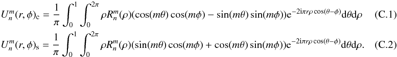 In both cases, the integral of the term sin(mθ) between 0 and 2π vanishes. Moreover, using the definition of the Bessel functions, we have
  (C.3)Substituting this expression into the two previous equations while using properties of the Bessel functions (Gradshteyn & Ryzhik 1994), and the radial result for the direct mth order Hankel transform Hm (see Eq. (B.7)), we finally obtain
  (C.4)
(C.4)
Appendix D: Expression of the V function (Fraunhofer diffraction)
In the classical Nijboer-Zernike theory without defocus the expression of the Vn,m is given directly by  (D.1)With the VVC, the coronagraphic pupil expression is given by the inverse lp + m order Hankel transform of the Bessel function included in the ,
 ![Mathematical equation: \appendix \setcounter{section}{4} \begin{eqnarray} && \Pi_{\rm c}(\rho,\theta)=2\pi^2 {\rm i}^m (-1)^{(n+m)/2} H_{l_{\rm p}\pm m}^{-1} \left[ \frac{J_{n+1}(2\pi r )} {2\pi r } {\rm e}^{{\rm i} (l_{\rm p} \phi-\pi/2)} \left\{ \begin{array}{l} \cos (m\phi)\\ \sin (m\phi)\\ \end{array} \right. \right]\\ && \Pi_{\rm c}(\rho,\theta)=2\pi^2 {\rm i}^m (-1)^{(n+m)/2} \frac{1}{\pi} \int_{0}^{+\infty} \int_{0}^{2\pi} \frac{J_{n+1}(2\pi r)} {2\pi r} {\rm e}^{{\rm i}(l_{\rm p} \phi-\pi/2)} \left\{ \begin{array}{l} \cos (m\phi)\\ \sin (m\phi)\\ \end{array} \right. {\rm e}^{{\rm i} 2\pi r \rho \cos(\phi-\theta)} {\rm d}\phi \: r{\rm d}r \nonumber \end{eqnarray}](/articles/aa/full_html/2012/09/aa19614-12/aa19614-12-eq293.png) (D.2)
(D.2)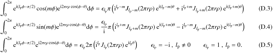 With lp even (necessary conditions to obtain the VVC coronagraphic effect), we have
 ![Mathematical equation: \appendix \setcounter{section}{4} \begin{eqnarray} &&\Pi_{\rm c}(\rho,\theta)={\rm i}^m \zeta_{n,m}^{l_{\rm p}}(\rho,\theta)_{\rm c/s} \\ &&\zeta_{n,m}^{l_{\rm p}}(\rho,\theta)_{\rm c}=\frac{\epsilon_{l_{\rm p}}} {2} 2\pi (-1)^{(n+m)/2} \int_{0}^{+\infty} J_{n+1}(2\pi r) \left[{\rm i}^{l_{\rm p}-m} \:{\rm e}^{{\rm i}(l_{\rm p}-m)\theta} J_{l_{\rm p}-m}(2 \pi r \rho) + {\rm i}^{l_{\rm p}+m} \:{\rm e}^{{\rm i}(l_{\rm p}+m)\theta} J_{l_{\rm p}+m}(2 \pi r \rho)\right] {\rm d}r \nonumber \\ &&\zeta_{n,m}^{l_{\rm p}}(\rho,\theta)_{\rm s}=\frac{\epsilon_{l_{\rm p}}} {2{\rm i}} 2\pi (-1)^{(n+m)/2} \int_{0}^{+\infty} J_{n+1}(2\pi r) \left[{\rm i}^{l_{\rm p}+m} \: {\rm e}^{{\rm i}(l_{\rm p}+m)\theta} J_{l_{\rm p}+m}(2 \pi r \rho) - {\rm i}^{l_{\rm p}-m} \:{\rm e}^{{\rm i}(l_{\rm p}-m)\theta} J_{l_{\rm p}-m}(2 \pi r \rho)\right] {\rm d}r \nonumber\\ && R_{n}^{|m|}(\rho)=(-1)^{(n-|m|)/2} \: 2\pi \int_0^{+\infty} J_{n+1}(2\pi r)J_{|m|}(2\pi \rho r) {\rm d}r \qquad 0\leq\rho<d_{\rm c} \nonumber \\ &&\zeta_{n,m}^{l_{\rm p}}(\rho,\theta)_{\rm c}=\frac{\epsilon_{l_{\rm p}}} {2} (-1)^{l_{\rm p}/2} {\rm i}^{l_{\rm p}-m}\: {\rm e}^{{\rm i} l_{\rm p}\theta}\: \left[R_n^{|l_{\rm p}+m|}(\rho) \: {\rm e}^{{\rm i}m\theta} + R_n^{|l_{\rm p}-m|}(\rho) \: {\rm e}^{-{\rm i}m\theta} \right]\quad (0<\rho<d_{\rm c})\nonumber\\ &&\zeta_{n,m}^{l_{\rm p}}(\rho,\theta)_{\rm s}=\frac{\epsilon_{l_{\rm p}}} {2 {\rm i}} (-1)^{l_{\rm p}/2} {\rm i}^{l_{\rm p}-m}\: {\rm e}^{{\rm i} l_{\rm p}\theta}\: \left[R_n^{|l_{\rm p}+m|}(\rho) \: {\rm e}^{{\rm i}m\theta} - R_n^{|l_{\rm p}-m|}(\rho) \: {\rm e}^{-{\rm i}m\theta}\right]\quad (0<\rho<d_{\rm c})\nonumber\\ &&\zeta_{n,m}^{l_{\rm p}}(\rho,\theta)_{m=0}= \epsilon_{l_{\rm p}} (-1)^{l_{\rm p}/2} {\rm i}^{l_{\rm p}} \: {\rm e}^{{\rm i} l_{\rm p}\theta}\: \left[R_n^{|l_{\rm p}|}(\rho) \right]\quad (0<\rho<d_{\rm c}) . \end{eqnarray}](/articles/aa/full_html/2012/09/aa19614-12/aa19614-12-eq295.png) Outside the coronagraphic pupil geometric area, it is necessary to change variables in the integrals to ensure a proper convergence: n → lp ± m lp ± m → n + 2 ρ → 1/ρ.
Outside the coronagraphic pupil geometric area, it is necessary to change variables in the integrals to ensure a proper convergence: n → lp ± m lp ± m → n + 2 ρ → 1/ρ.
For n = 0,m = 0,lp = 2: 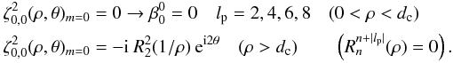 (D.8)These last two results correct typos in Eq. (C.7) in the appendix of (Mawet et al. 2005) for n = 0,m = 0.
 |
Fig. D.1 Input classical Zernike |
 |
Fig. D.2
|

 |
Fig. D.3
|

 |
Fig. D.4 Uv(r,φ),lp = ± 2 functions in the coronagraphic image plane for the 10 Zernike polynomials (Z2 − Z11). Top: lp = + 2, Bottom: lp = −2. The vertical solid line separates the real part from the imaginary part of the two Uv(r,φ) functions. |
Note that the pupil integration on the ρ coordinate is applied between 0 and dc because of the presence of the Lyot stop,  (D.9)To retrieve the coronagraphic amplitude residual in the final imaging plane, we use the direct lp + m order Hankel transform of the coronagraphic pupil plane,
 ![Mathematical equation: \appendix \setcounter{section}{4} \begin{eqnarray} &&U_v (r,\phi)= H_{l_{\rm p}\pm m} \left[\Pi_{\rm c}(\rho,\theta) \right]\\ &&U_v (r,\phi)_{\rm c}=\epsilon_{l_{\rm p}} \sum_{n,m} \beta_n^m(d_{\rm c})_{\rm c} \: 2{\rm i}^{m} (-1)^{(n+m)/2} \: {\rm e}^{{\rm i} l_{\rm p}\phi} \frac{J_{n+1}(2\pi r)} {2\pi r} C_m(\phi) \qquad U_v (r,\phi)_{\rm s}=\epsilon_{l_{\rm p}} \sum_{n,m} \beta_n^m(d_{\rm c})_{\rm s} \: 2{\rm i}^{m} (-1)^{(n+m)/2} \: {\rm e}^{{\rm i} l_{\rm p}\phi} \frac{J_{n+1}(2\pi r)} {2\pi r} S_m(\phi)\nonumber\\ &&C_m(\phi)=\left( {\rm e}^{{\rm i} m \theta} + {\rm e}^{-{\rm i} m \theta} \right)/2 \qquad S_m(\phi)=\left({\rm e}^{{\rm i} m \theta} - {\rm e}^{-{\rm i} m \theta}\right)/2{\rm i} .\nonumber \end{eqnarray}](/articles/aa/full_html/2012/09/aa19614-12/aa19614-12-eq307.png) (D.10)We do not simplify
(D.10)We do not simplify  with 2.cos(mθ) or 2i.sin(mθ) because when n = m the Zernike polynomial
  or
or  ,
,  (D.11)
-
m = 0 − → Cm(φ) = 1 Sm(φ) = 0
0 < m < n − → Cm(φ) = cos(mφ) Sm(φ) = sin(mφ)
m = n − → Cm(φ) = (cos(mφ) − iSign(lp)sin(mφ))/2 Sm(φ) = (sin(mφ) + iSign(lp)cos(mφ))/2.
In the final imaging plane, a VVC device of order lp adds a POAM lp on the incoming residual light (Poynting 1909; Allen et al. 1999).
Appendix E: Polychromatic V expression
In the broadband case, we can use a polychromatic set of functions  to enable a better complex amplitude aberration retrieval. The main effect is to broaden the monochromatic
  set of functions and to decrease the contrast of the Bessel Jn + 1 rings of the coronagraphic images. These two effects can be implemented with a simple Gaussian convolution of the monochromatic functions,
  (E.1)Using the two following relations in the convolution
 ![Mathematical equation: \appendix \setcounter{section}{5} \begin{equation} \label{polycc1} \frac{J_{n+1}(2\pi(r-x))} {2\pi(r-x)}= \frac{1}{2(n+1)} \left[ J_n(2\pi(r-x)) + J_{n+2}(2\pi(r-x))\right] \qquad \qquad J_n(2\pi(r-x))=\sum_{k=0}^{+\infty} {J_{n+k}(2\pi r).J_{k}(2\pi x)} , \end{equation}](/articles/aa/full_html/2012/09/aa19614-12/aa19614-12-eq323.png) (E.2)we obtain
(E.2)we obtain ![Mathematical equation: \appendix \setcounter{section}{5} \begin{equation} \label{polycc2a} \int_0^{+\infty} {{\rm e}^{-x^2/2\sigma_g^2} \frac{J_{n+1}(2\pi(r-x))} {2\pi(r-x)} {\rm d}x}= \frac{1}{2(n+1)}\sum_{k=0}^{+\infty} {\int_0^{+\infty} {{\rm e}^{-x^2/2\sigma_g^2} J_{k}(2\pi x) \left[ J_{n+k}(2\pi r) + J_{n+2+k}(2\pi r)\right] {\rm d}x}} . \end{equation}](/articles/aa/full_html/2012/09/aa19614-12/aa19614-12-eq324.png) (E.3)Following Gradshteyn & Ryzhik (1994), p1094, the infinite integral can be calculated analytically,
(E.3)Following Gradshteyn & Ryzhik (1994), p1094, the infinite integral can be calculated analytically, 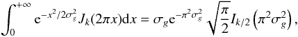 (E.4)where Ik/2 is the Bessel I function. Note that the two Bessel J functions can be compacted as follows:
 ![Mathematical equation: \appendix \setcounter{section}{5} \begin{equation} \label{polycc3} \left[ J_{n+k}(2\pi r) + J_{n+2+k}(2\pi r)\right]= 2 (n+k+1) \frac{J_{n+k+1}(2\pi r)} {2\pi r}\cdot \end{equation}](/articles/aa/full_html/2012/09/aa19614-12/aa19614-12-eq327.png) (E.5)The polychromatic set of functions then becomes
(E.5)The polychromatic set of functions then becomes  (E.6)The Bessel I function decreases quickly with respect to the k variable. Therefore, the discrete summation on the first 20 to 30 k coefficients is sufficient to retrieve the final function to an accuracy of 10-12. Note that the βn,m coefficients retrieved in the polychromatic case correspond to the worst attenuation factor at the shortest wavelength.
Appendix F: Energy conservation
Each mode must be normalized by its intensity for a proper retrieval analysis,  (F.1)
(F.1)![Mathematical equation: \appendix \setcounter{section}{6} \begin{equation} \label{modes_E2} E(V_{n,m}^{l_{\rm p}})=2 r^{2n+2}_{\rm max} \pi^{2n+2} \frac{\Gamma[2n+2]}{\Gamma[n+2]^2\Gamma[2n+3]} {_2}F_3 \left(n+1,n+3/2;n+2,n+2,2n+3;4\pi^2 r^2_{\rm max}\right) \qquad E(V_{0,0}^{l_{\rm p}})_{r_{\rm max}\rightarrow +\infty} = 1. \end{equation}](/articles/aa/full_html/2012/09/aa19614-12/aa19614-12-eq332.png) (F.2)Similarly, we obtain in the polychromatic case
(F.2)Similarly, we obtain in the polychromatic case  (F.3)
(F.3)
Appendix G: Analytical vs. Fourier simulations
We performed numerical simulations to compare the robustness of the analytical functions in the monochromatic case to the classical FFT computations. These simulations were performed on 2K × 2K arrays using the “super-resolution” method presented in Sect. 7.1. A χ2 and Err(σA) are calculated for each Zernike on a box centered on the coronagraphic image of 256 × 256 pixel square. We assume that each function is optimized in terms of sampling, 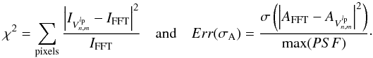 (G.1)The χ2 is normalized to the number of pixels inside an annulus centered on the mode: typically, a χ2 < 1 is considered as good. The following Figs. G.1 and G.2 show structuring features as a function of the Zernike mode parity number m.
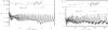 |
Fig. G.1 Comparison between Fourier simulations for each Zernike polynomial (2-860) and |
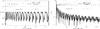 |
Fig. G.2 Comparison between Fourier simulations for each Zernike polynomial (2-860) and |
Appendix H: Expression of the pupil function in Fresnel diffraction ( )
)
H.1. Circular pupil
This appendix presents the calculation of the Fresnel diffraction of the coronagraphic pupil  . Indeed, due to the uncertainty of the Lyot stop position, the diffracted field must be treated according to the Fresnel diffraction theory,
 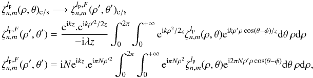 (H.1)where k = 2π/λ, z is the Fresnel distance propagation, and is the Fresnel number.
Inside the pupil plane, we have ![Mathematical equation: \appendix \setcounter{section}{8} \begin{eqnarray} \label{fr2a} &&\zeta_{n,m}^{l_{\rm p},F}(\rho',\theta')_{\rm c}=\frac{P_F^{l_{\rm p}}} {2}\int_{0}^{d_{\rm c}} {\rm e}^{{\rm i} \pi N \rho^{2}} \left[R_n^{|l_{\rm p}+m|}(\rho) J_{l_{\rm p} + m}(2 \pi N \rho \rho' )\: {\rm e}^{{\rm i}m\theta'} + R_n^{|l_{\rm p}-m|}(\rho) J_{l_{\rm p}-m}(2 \pi N \rho \rho' )\: {\rm e}^{-{\rm i}m\theta'} \right] \rho {\rm d}\rho\\ &&\zeta_{n,m}^{l_{\rm p},F}(\rho',\theta')_{\rm s}=\frac{P_F^{l_{\rm p}}} {2i}\int_{0}^{d_{\rm c}} {\rm e}^{{\rm i} \pi N \rho^{2}} \left[R_n^{|l_{\rm p}+m|}(\rho) J_{l_{\rm p} + m}(2 \pi N \rho \rho' )\: {\rm e}^{{\rm i}m\theta'} - R_n^{|l_{\rm p}-m|}(\rho) J_{l_{\rm p}-m}(2 \pi N \rho \rho' )\: {\rm e}^{-{\rm i}m\theta'} \right] \rho {\rm d}\rho~~~~~~~~~~~~~~~~~~~~~~~~\\ &&P_F^{l_{\rm p}}(\rho',\theta')=2{\rm i}\pi N {\rm e}^{{\rm i} k z}.{\rm e}^{{\rm i} \pi N \rho'^{2}} \epsilon_{l_{\rm p}} (-1)^{l_{\rm p}/2} {\rm i}^{l_{\rm p}-m}\: {\rm e}^{{\rm i}l_{\rm p}\theta'} .\nonumber \end{eqnarray}](/articles/aa/full_html/2012/09/aa19614-12/aa19614-12-eq345.png) Outside the pupil plane, we have
Outside the pupil plane, we have ![Mathematical equation: \appendix \setcounter{section}{8} \begin{eqnarray} \label{fr2a2} &&\zeta_{n,m}^{l_{\rm p},F}\left(\rho',\theta'\right)_{\rm c}=\frac{P_F^{l_{\rm p}}} {2}\int_{d_{\rm c}}^{+\infty} {\rm e}^{{\rm i} \pi N \rho^{2}} \left[R_{|l_{\rm p}+m|}^{n+2}\left(\frac{1}{\rho}\right) J_{l_{\rm p} + m}\left(2 \pi N \rho \rho' \right)\: {\rm e}^{{\rm i}m\theta'} + R_{|l_{\rm p}-m|}^{n+2}\left(\frac{1}{\rho}\right) J_{l_{\rm p}-m}\left(2 \pi N \rho \rho' \right)\: {\rm e}^{-{\rm i}m\theta'} \right] \rho {\rm d}\rho\\ &&\zeta_{n,m}^{l_{\rm p},F}\left(\rho',\theta'\right)_{\rm s}=\frac{P_F^{l_{\rm p}}} {2i}\int_{d_{\rm c}}^{+\infty} {\rm e}^{{\rm i} \pi N \rho^{2}} \left[R_{|l_{\rm p}+m|}^{n+2}\left(\frac{1}{\rho}\right) J_{l_{\rm p} + m}\left(2 \pi N \rho \rho' \right)\: {\rm e}^{{\rm i}m\theta'} - R_{|l_{\rm p}-m|}^{n+2}\left(\frac{1}{\rho}\right) J_{l_{\rm p}-m}\left(2 \pi N \rho \rho' \right)\: {\rm e}^{-{\rm i}m\theta'} \right] \rho {\rm d}\rho .~~~~~~~~~~~~~ \end{eqnarray}](/articles/aa/full_html/2012/09/aa19614-12/aa19614-12-eq346.png) Inside the pupil plane, we have two terms: the Zernike polynomials, and a pupil edge effect. Here, we make use of Babinet’s principle of complementary screens to express the second integral as a classical Fresnel diffraction between 0 to dc,
Inside the pupil plane, we have two terms: the Zernike polynomials, and a pupil edge effect. Here, we make use of Babinet’s principle of complementary screens to express the second integral as a classical Fresnel diffraction between 0 to dc,  (H.6)
(H.6) The first integral can be calculated with all Zernike polynomials:
 ![Mathematical equation: \appendix \setcounter{section}{8} \begin{eqnarray} \label{fr3b} &&F_{n,m}^{l_{\rm p}}( \rho',1)= \sum^{\frac{n-|m+l_{\rm p}|}{2}}_{s=0} C_z(n,|m+l_{\rm p}|,s) \int_{0}^{+\infty} \: \rho^{n-2s+1 } {\rm e}^{{\rm i} \pi N \rho^{2}} J_{l_{\rm p} + m}(2 \pi N \rho \rho' ) {\rm d}\rho \\ &&F_{n,m}^{l_{\rm p}}( \rho',1)= \!\! \sum^{\frac{n-|m+l_{\rm p}|}{2}}_{s=0}\!\! C_z(n,|m+l_{\rm p}|,s) (-{\rm i}\pi N)^{(|l_{\rm p}+m|-n-2+2s)/2} \cdot \frac{\Gamma[(\frac{|l_{\rm p}+m|+n+2-2s} {2}]*\rho'^{|l_{\rm p}+m|}}{\Gamma[(|l_{\rm p}+m|+1]} {_1}F_1\left(\frac{|l_{\rm p}+m|+n+2-2s} {2},|l_{\rm p}+m|+1,-{\rm i}\pi N \rho'^2 \right), \nonumber \end{eqnarray}](/articles/aa/full_html/2012/09/aa19614-12/aa19614-12-eq349.png) (H.7)where
(H.7)where  is the confluent hypergeometric function.
The second integral only represents a diffraction effect to the Jlp order, 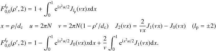 (H.8)We define the Lommel functions of two variable generally used in the Fresnel diffraction of a circular screen (Born & Wolf 1999):
 ![Mathematical equation: \appendix \setcounter{section}{8} \begin{eqnarray} \label{fr3d} && U_n(u,v)=\sum_{j=0}^{+\infty} (-1)^j \left(\frac{u} {v}\right)^{n+2j} J_{n+2j}(v) \qquad V_n(u,v)=\sum_{j=0}^{+\infty} (-1)^j \left(\frac{v} {u}\right)^{n+2j} J_{n+2j}(v) \\ \label{fr3e} && \int_{0}^{1} {\rm e}^{{\rm i} x^2 u/2} J_0(vx) x {\rm d}x = \frac{{\rm e}^{{\rm i} u/2}} {u} \left(U_1(u,v)-{\rm i} U_2(u,v) \right) \qquad \frac{2} {v} \int_{0}^{1} {\rm e}^{{\rm i} x^2 u/2} J_1(vx) {\rm d}x =\frac{2} {uv}\left({\rm e}^{-{\rm i}v^2/2u} + \left( J_0(v)- V_0(u,v)- {\rm i} V_1(u,v) \right) {\rm e}^{{\rm i} u/2} \right)\nonumber\\[2mm] &&F_{0,0}^{l_{\rm p}}( \rho',2)=1+\frac{2 {\rm e}^{-{\rm i}v^2/2u}} {uv}+ \frac{{\rm e}^{{\rm i} u/2}} {u} \left(\frac{2 J_0(v)} {v}- \frac{2 V_0(u,v)- 2{\rm i} V_1(u,v)}{v} - U_1(u,v) + {\rm i} U_2(u,v) \right) \end{eqnarray}](/articles/aa/full_html/2012/09/aa19614-12/aa19614-12-eq353.png)
 (H.11)We include the diaphragm edge effect due to the Fresnel propagation only in the first term
  . The coronagraphic pupil with Fresnel propagation thus becomes
 ![Mathematical equation: \appendix \setcounter{section}{8} \begin{eqnarray} \label{fr4} &&\Pi_{\rm c}^F(\rho',\theta')_{\rm c}=2{\rm i}\pi N \epsilon_{l_{\rm p}} {\rm e}^{{\rm i} k z} \sum_{n,m} \beta_n^m(d_{\rm c}) {\rm e}^{{\rm i} \pi N \rho'^{2}} (-1)^{l_{\rm p}/2} {\rm i}^{l_{\rm p}}\: {\rm e}^{{\rm i}l_{\rm p}\theta'} \frac{1} {2} \left[F_{n,m}^{l_{\rm p}}( \rho')\: {\rm e}^{{\rm i}m\theta'} +F_{n,-m}^{l_{\rm p}}( \rho') {\rm e}^{-{\rm i}m\theta'}\right]\\ &&\Pi_{\rm c}^F(\rho',\theta')_{\rm s}=2{\rm i}\pi N \epsilon_{l_{\rm p}} {\rm e}^{{\rm i} k z} \sum_{n,m} \beta_n^m(d_{\rm c}) {\rm e}^{{\rm i} \pi N \rho'^{2}} (-1)^{l_{\rm p}/2} {\rm i}^{l_{\rm p}}\: {\rm e}^{{\rm i}l_{\rm p}\theta'} \frac{1} {2{\rm i}}\left[F_{n,m}^{l_{\rm p}}( \rho')\: {\rm e}^{{\rm i}m\theta'} +F_{n,-m}^{l_{\rm p}}( \rho'){\rm e}^{-{\rm i}m\theta'}\right] .~~~~~~~~~~~~~ \end{eqnarray}](/articles/aa/full_html/2012/09/aa19614-12/aa19614-12-eq356.png)
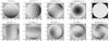 |
Fig. H.1
|

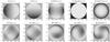 |
Fig. H.2
|

H.2. Annular pupil
A telescope with a central obscuration ϵ must be treated with annular Zernike polynomials, but the central obscuration creates a strong diffraction phenomenon at the edge of the pupil (1 > ρ > ϵ). The effect of the optical aberration (n ≠ 0, m ≠ 0) gives  the
the  must be calculated taking into account the diffraction of the central obscuration. The
  function included in the
  can thus be written
  (H.14)
-
 : The Fresnel diffraction of the outer edge of the pupil as calculated previously
  : The Fresnel diffraction of the the central obscuration edge inside the pupil
 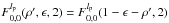 , ρ′ > ϵ
 : Starlight diffraction on a perfect circular pupil.
![Mathematical equation: \appendix \setcounter{section}{8} \begin{equation} \label{fr_an3} F_{0,0}^{l_{\rm p}}( \rho',\epsilon,3)=\int_{0}^{+\infty} \: \rho^{1-l_{\rm p}} {\rm e}^{{\rm i} \pi N (\rho/\epsilon)^{2}} J_{l_{\rm p} }(2 \pi N \rho \rho'/\epsilon ) {\rm d}\rho \quad \longrightarrow \quad F_{0,0}^{l_{\rm p}}( \rho',\epsilon,3)=\frac{{\rm i}^{l_{\rm p}/2}\epsilon^{l_{\rm p}} \Gamma[l_{\rm p}/2+2]}{2(\pi N)^{l_{\rm p}/2}\rho'^{l_{\rm p}}} {_1}F_1 \left(l_{\rm p}/2+2,3,-{\rm i}\pi N \epsilon^2/\rho'^2 \right) \end{equation}](/articles/aa/full_html/2012/09/aa19614-12/aa19614-12-eq374.png) (H.15)
(H.15)
Appendix I: Scaled radial Zernike polynomial
ming Dai (2006) gives the Zernike coefficients of the scaled pupil as a function of those of the unscaled pupil,  (I.1)This expression is somewhat complicated. In this Appendix, we propose to calculate the scaled coefficients in a simpler way. The main idea is to transform
  with the coronagraphic diaphragm dc < 1. We need to calculate a new orthogonality relation:
 ![Mathematical equation: \appendix \setcounter{section}{9} \begin{eqnarray} \label{new_orth} && D_{nn'}^m(d_{\rm c})=\int_0^1 R_n^m(\rho)R_{n'}^m(\rho d_{\rm c})\rho {\rm d}\rho \qquad \left(\forall n\:,\:n'=m,m+2,... \right) \quad\longrightarrow\quad \beta_n^m(d_{\rm c})= 2(n+1) \sum_{n'} \beta_{n'}^m \cdot D_{nn'}^m(d_{\rm c}) \\ \label{new_sc1} && R_{n'}^m(\rho d_{\rm c})=(-1)^{(n'-m)/2} \int_0^{+\infty} J_{n'+1}(r)J_{m}(\rho d_{\rm c} r) {\rm d}r \qquad 0\leq\rho<1 \nonumber \\ && D_{nn'}^m(d_{\rm c})=(-1)^{(n'-m)/2} \int_0^{+\infty}J_{n'+1}(r) \left[ \int_0^1 R_{n}^m(\rho) J_{m}(\rho d_{\rm c} r) \rho {\rm d}\rho \right]{\rm d}r\nonumber \\ && D_{nn'}^m(d_{\rm c})=(-1)^{(n'+n-2m)/2} \int_0^{+\infty} \frac{J_{n'+1}(r).J_{n+1}(d_{\rm c} r)} {d_{\rm c} r} {\rm d}r\nonumber \end{eqnarray}](/articles/aa/full_html/2012/09/aa19614-12/aa19614-12-eq377.png) (I.2)
(I.2)![Mathematical equation: \appendix \setcounter{section}{9} \begin{eqnarray} \label{new_sc2} &&\frac{J_{n+1}(d_{\rm c} r)} {d_{\rm c} r} = \frac{J_{n}(d_{\rm c} r)+J_{n+2}(d_{\rm c} r)} {2(n+1)}\nonumber \\[2mm] && D_{nn'}^m(d_{\rm c})=\frac{(-1)^{(n'+n-2m)/2}} {2(n+1)} \left[\int_0^{+\infty}J_{n'+1}(r) J_{n}(d_{\rm c} r) {\rm d}r + \int_0^{+\infty}J_{n'+1}(r)J_{n+2}(d_{\rm c} r) {\rm d}r \right]\nonumber \\[2mm] && D_{nn'}^m(d_{\rm c})=\frac{R_{n'}^n(d_{\rm c})-R_{n'}^{n+2}(d_{\rm c})} {2(n+1)} \cdot \end{eqnarray}](/articles/aa/full_html/2012/09/aa19614-12/aa19614-12-eq378.png) (I.3)Finally, the scaled can be calculated more easily than with the complicated formula in ming Dai (2006) and we obtain
(I.3)Finally, the scaled can be calculated more easily than with the complicated formula in ming Dai (2006) and we obtain ![Mathematical equation: \appendix \setcounter{section}{9} \begin{equation} \label{new_orth_f} \beta_n^m(d_{\rm c})=\sum_{n'} \beta_{n'}^m \cdot \left[ R_{n'}^n(d_{\rm c})-R_{n'}^{n+2}(d_{\rm c}) \right] \qquad n=m,m+2,... \quad n'=n,n+2,... \end{equation}](/articles/aa/full_html/2012/09/aa19614-12/aa19614-12-eq379.png) (I.4)Similarly,
(I.4)Similarly,  (I.5)In Eq. (I.3), we commute n and n′
![Mathematical equation: \appendix \setcounter{section}{9} \begin{equation} \label{new_sc3} D_{nn'}^{'m}(d_{\rm c})=\frac{R_{n}^{n'}(d_{\rm c})-R_{n}^{n'+2}(d_{\rm c})} {2(n'+1)}\quad \longrightarrow \quad \beta_n^m= (n+1) \sum_{n'} \beta_{n'}^m(d_{\rm c}) \cdot \frac{\left[ R_{n}^{n'}(d_{\rm c})-R_{n}^{n'+2}(d_{\rm c}) \right]} {(n'+1)} \qquad n=m,m+2,... \end{equation}](/articles/aa/full_html/2012/09/aa19614-12/aa19614-12-eq383.png) (I.6)
(I.6)
Appendix J: Vortex phase-mask nulling limitation
This section presents the main mathematical properties of an imperfect vortex device owing to manufacturing defects. In real life, the optical vortex phase-mask presents three problems:
-
The phase-shift error with respect to π (chromaticity).
-
The region in the center of the mask presents a deviation from the overall large-scale pattern, called region of disorientation.
-
The finite size of the mask in the coronagraphic image plane.
J.1. The phase-shift error
For manufacturing defects, a VVC MV can be modeled in the following way:  where Ts and Tp are the polarization transmittance for s and p polarization, respectively (depolarization issue), Δφ is the local phase retardance deviation around π with respect to the wavelength. In these conditions, the radial mode templates are modified by the CM,γM terms. If CM = 1,γM = 0 the output image intensity is completely described by the classical NZ theory (without coronagraph). In the general case, the complete coronagraphic intensity development becomes more complicated and shows several coupled terms such as
  Generally, the term CM ≈ 0. Moreover, remember that the first step of the wavefront retrieval process only uses the linear terms. A simple correction of the vortex phase e ± ilpφ by γM allows us to reject all CM Zernike polynomial terms in the coefficient. The CM term can be seen as no POAM (Poynting 1909; Allen et al. 1999) added by the vortex coronagraph. Unfortunately, a few part of aberrations pass through the coronagraphic device without speckle modulation because of the Pancharatnam topological charge lp effect.
J.2. The central region of disorientation
The finite mask extension is easily taking into account in our Nijboer-Zernike development by cutting high-order rings of the Bessel function in the functions. The central region of disorientation is the most important effect on of the coronagraphic rejection. Indeed, most of the stellar energy to be suppressed will fall on it. The uncertainty for the diameter of the central region of disorientation allows us to use a simplistic hole model. The nulling factor can be calculated with the modified NZ theory and the maximum nulling factor Nv is given by  (J.3)where s is the radius of the disorientation region expressed in λ/d units.
Covering this central region of disorientation with an opaque mask (small Lyot-like coronagraph) allows us to reach the chromatic limit, but create diffraction effects at the edge of the Lyot stop. In our NZ simulation, we can take the presence of this diffraction into account by changing the  function (in the perfect case:
  ). Indeed, the maximum coronagraphic rejection without optical aberration is given by the term,
 ![Mathematical equation: \appendix \setcounter{section}{10} \begin{eqnarray} \label{null_int2} &&\zeta_{0,0}^{l_{\rm p}}(\rho,s_1,s_2,\theta)= \epsilon_{l_{\rm p}} (-1)^{l_{\rm p}/2} {\rm i}^{l_{\rm p}} \:{\rm e}^{{\rm i}l_{\rm p}\theta} 2\pi \int_{0}^{+\infty} \left[ \Pi(0,s_2) - \Pi(0,s_1)\right] J_1(2\pi r) J_{l_{\rm p}}(2\pi r \rho) {\rm d}r \\ &&\zeta_{0,0}^{l_{\rm p}}(\rho,s_1,s_2,\theta)=H_{l_{\rm p}}\left[J_1(2\pi r)\right] \otimes H_{l_{\rm p}}\left[\Pi(0,s_2) - \Pi(0,s_1)\right]\nonumber \\[2mm] &&H_{l_{\rm p}}\left[\Pi(0,s)\right]=\frac{2 (\pi s)^{l_{\rm p}+1}\rho^{l_{\rm p}}} {\Gamma[l_{\rm p}+2]} {_2}F_1\left(\frac{l_{\rm p}+2}{2}, \frac{l_{\rm p}+3}{2},l_{\rm p}+1, ({\rm i}\pi s \rho)^2\right)\qquad \qquad H_{l_{\rm p}}\left[J_1(2\pi r)\right]=\epsilon_{l_{\rm p}} (-1)^{l_{\rm p}/2} {\rm i}^{l_{\rm p}} \:{\rm e}^{{\rm i}l_{\rm p}\theta} R_0^{|l_{\rm p}|}(\rho)\nonumber \\[2mm] \label{null_int22} &&\zeta_{0,0}^{l_{\rm p}}(\rho,s_1,s_2,\theta)=2 \epsilon_{l_{\rm p}} (-1)^{l_{\rm p}/2} {\rm i}^{l_{\rm p}} \:{\rm e}^{{\rm i}l_{\rm p}\theta} \frac{\rho^{l_{\rm p}}}{\Gamma[l_{\rm p}+2]} \Pi(0,1) \\ &&\quad \times \left[(\pi s_2)^{l_{\rm p}+1} {_2}F_1\left(\frac{l_{\rm p}+2}{2}, \frac{l_{\rm p}+3}{2},l_{\rm p}+1, ({\rm i}\pi s_2 \rho)^2\right) - (\pi s_1)^{l_{\rm p}+1} {_2}F_1\left(\frac{l_{\rm p}+2}{2}, \frac{l_{\rm p}+3}{2},l_{\rm p}+1, (i\pi s_1 \rho)^2\right)\right] , \nonumber \end{eqnarray}](/articles/aa/full_html/2012/09/aa19614-12/aa19614-12-eq402.png) where the vortex mask extent is [s1,s2] , Π(0,1) is the unit box function and is the Gauss hypergeometric function. The
where the vortex mask extent is [s1,s2] , Π(0,1) is the unit box function and is the Gauss hypergeometric function. The  function inside the pupil can be approximated by a simple parabolic function: 10-5ρ2 0 < ρ < 1 lp = 2 as a simple defocus.
Appendix K: Lyot stop optimization
The diaphragm in the coronagraphic pupil plane must be optimized to obtain a good ratio between the nulling factor and the planet throughput attenuation because of this Lyot stop. The total nulling factor ϵc can be defined as follows:  (K.1)The coronagraphic pupil presents in real life three different diffraction patterns: a smooth ρ2 residual light in the pupil owing to the small Lyot coronograph in the center (pseudo-apodization), a light modulation inside the pupil owing to optical aberrations, and finally a strong light gradient in the edge of the pupil with diffraction oscillations.
K.1. Residual optical aberrations
The diaphragm optimization in the presence of aberrations can be easily calculated as follows:  (K.2)where 1/npw is the power spectral density of the optical aberrations. We consider two extreme cases: pw = 1 (strong aberration residuals on an adaptive optics for example) and pw = 2 (optical polishing). Results are given in the two following figures (Fig. K.1):
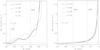 |
Fig. K.1 Variation of the residual energy (dEp/dx) in the residual optical aberrations as a function of the number of Zernike polynomials used (nz – without the piston term) and the power spectral density 1/npw. The figure shows two diaphragm values: when the gain is maximum and when it is equal to zero. The figure in 1/n presents strong residual oscillations owing to low-order aberrations. |
K.2. Diffraction oscillations
We need to calculate the  function (including ) previously given in Appendix H. In the visible/near-infrared, these oscillations are generally limited to the region 0.8 < ρ < 1 (see numerical simulations in Riaud & Schneider 2007).
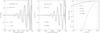 |
Fig. K.2 Fresnel diffraction of the Lyot stop with an optical vortex coronagraph. We present the real and the imaginary parts of the |
To minimize the Fresnel residual diffraction in the coronagraphic pupil plane, it is necessary to increase the Fresnel number N. For high-contrast imaging devoted to the research of telluric planets around nearby stars (10-10 contrast level), the diaphragm (86%) has to be positioned with ± 50 μm accuracy with respect to the real pupil position (N > 10 000) along the optical axis. To simplify the aberration retrieval process, the only contains pseudo-apodization pattern owing to the small Lyot dot in the center of the mask and not the one caused by the propagation of the Lommel function of two variables given by the term. Indeed, these functions are somewhat negligible if we use the proper Lyot stop diameter (86% in the case presented here) and a good diaphragm position.
K.3. Annular pupil
The case of the annular pupil is relatively simple, because all simulations already given in the previous section can be used for a larger diameter of the Lyot stop. Concerning the optimization of the smaller diameter of the Lyot stop, the value is completely governed by the starlight diffraction of the telescope obscuration ( ∝ ρ − lp). For an obscuration ϵ = 0.14 (Very Large Telescope) an inner radius (din) of 0.3 and lp = ± 2 allows one to obtain a total nulling factor of |ϵ2(ln(din) − ln(ϵ))|2 ≈ 1/4500.
Appendix L: Spider diffraction in the Fresnel mode
A telescope with a central obscuration possesses a complex spider to hold the secondary mirror. We present here the Fresnel development of the residual diffraction caused by a thin spider in the coronagraphic pupil with the vortex coronagraph.
First of all, we calculate this effect in the classical cartesian coordinates (x,y) taking into account the vortex term (eilpθ) and after that, we transform the result into the polar coordinates. We follow the Fresnel notation given in the previous analytical section: ρ → ρ′, θ → θ′, and now x → x′, y → y′. A spider is defined as follows: x is ( ± th/2) the thichness of the spider in radius unit and y is (ϵ to 1) the spider length. The spider is on azimuthal position θn. Generally, a telescope possesses three or four spiders. For the VLT-UT telescopes, we sum in amplitude the diffraction contribution of four different spiders: n = 1,2,3,4 with azimuthal angle of 109 degres. The Fresnel diffraction Un(x′,y′) of one spider becomes  (L.1)After some variable changes, we obtain the spider diffraction as a function of the modified Fresnel integrals C(ξ,lp) and S(ξ,lp)
 ![Mathematical equation: \appendix \setcounter{section}{12} \begin{equation} \label{spider2} U_n(x',y')=1-\frac{{\rm e}^{{\rm i} l_{\rm p} \theta_n}}{2{\rm i}} \left(\left[C(\xi_{x2},l_{\rm p})+{\rm i}S(\xi_{x2},l_{\rm p})\right]-\left[C(\xi_{x1},l_{\rm p})+{\rm i}S(\xi_{x1},l_{\rm p})\right] \right) \cdot \left(\left[C(\xi_{y2},l_{\rm p})+{\rm i}S(\xi_{y2},l_{\rm p})\right]-\left[C(\xi_{y1},l_{\rm p})+{\rm i}S(\xi_{y1},l_{\rm p})\right] \right) \end{equation}](/articles/aa/full_html/2012/09/aa19614-12/aa19614-12-eq440.png) (L.2)where
(L.2)where ![Mathematical equation: \appendix \setcounter{section}{12} \begin{eqnarray} \label{spider3} &&C(\alpha_{x/y},l_{\rm p})=\int_{0}^{\alpha_{x/y}} \cos\left(\pi/2\cdot \xi_{x/y}^2\right) \cos\left(l_{\rm p}\cdot {\rm ArcTan}\left(\frac{\xi_{y}\sqrt{(z\lambda/2)}+y'}{\xi_{x}\sqrt{(z\lambda/2)}+x'}\right)\right){\rm d}\xi_{x/y} \\[2mm] &&S(\alpha_{x/y},l_{\rm p})=\int_{0}^{\alpha_{x/y}} \sin\left(\pi/2\cdot \xi_{x/y}^2\right) \sin\left(l_{\rm p}\cdot {\rm ArcTan}\left(\frac{\xi_{y}\sqrt{(z\lambda/2)}+y'}{\xi_{x}\sqrt{(z\lambda/2)}+x'}\right)\right){\rm d}\xi_{x/y} .~~~~~~~~~~~~~~ \end{eqnarray}](/articles/aa/full_html/2012/09/aa19614-12/aa19614-12-eq441.png) These modified Fresnel integrals are relatively complicated in cartesian coordinates. Now, we use the polar coordinates to calculate this diffraction in a more convenient way:
These modified Fresnel integrals are relatively complicated in cartesian coordinates. Now, we use the polar coordinates to calculate this diffraction in a more convenient way: ![Mathematical equation: \appendix \setcounter{section}{12} \begin{eqnarray} \label{spider4} &&x \rightarrow \rho\sin(|\theta_n-\theta|) \quad y \rightarrow \rho \qquad x' \rightarrow \rho'\sin(|\theta_n-\theta'|) \quad y' \rightarrow \rho' \nonumber \\ &&U_n(\rho',\theta')=1-\frac{{\rm e}^{{\rm i} l_{\rm p} \theta_n}}{2{\rm i}} \left(\left[C(\xi_{s2},l_{\rm p})+{\rm i}S(\xi_{s2},l_{\rm p})\right]-\left[C(\xi_{s1},l_{\rm p})+{\rm i}S(\xi_{s1},l_{\rm p})\right] \right) \cdot \left(\left[C(\xi_{\rho2})+{\rm i}S(\xi_{\rho2})\right]-\left[C(\xi_{\rho1})+{\rm i}S(\xi_{\rho1})\right] \right) . \end{eqnarray}](/articles/aa/full_html/2012/09/aa19614-12/aa19614-12-eq442.png) (L.5)In this coordinate transform y depends only on ρ and the diffraction integral on ρ′ does not depend on the θ coordinate. The Fresnel integrals become
(L.5)In this coordinate transform y depends only on ρ and the diffraction integral on ρ′ does not depend on the θ coordinate. The Fresnel integrals become  In the coronagraphic pupil plane, we use a Lyot-stop for a proper starlight filtering, but we also notice that this diaphragm suppresses the Fresnel diffraction on the ρ′ axis. The spider creates only residual diffraction on the x′ coordinate. The Fresnel oscillations in the edges of the spider depend on the ρ′ and the θ′ coordinates. In these conditions, the modified Fresnel integrals must be simplified in the ArcTan() using exponential algebra for a fixed value of lp:
 ![Mathematical equation: \appendix \setcounter{section}{12} \begin{eqnarray} \label{spider6b} &&C(\xi_{\rm sn},l_{\rm p}=\pm 2)=\int_{0}^{\xi_{\rm sn}} \cos\left(\pi/2\cdot \xi^2\right) \left(\frac{4}{z\lambda \xi^2-\cos(2(|\theta_n-\theta'|))+\sqrt{8z\lambda}\xi \sin(|\theta_n-\theta'|)+3}-1 \right) {\rm d}\xi ~~~~~~~~~~~~~~~~~~~~~~~~~\\[2mm] &&S(\xi_{\rm sn},l_{\rm p}=\pm 2)=\int_{0}^{\xi_{\rm sn}} \sin\left(\pi/2\cdot \xi^2\right) \left(\frac{4\left(\sqrt{z\lambda/2}\xi+\sin(|\theta-n-\theta'|)\right)}{z\lambda \xi^2-\cos(2(|\theta_n-\theta'|))+\sqrt{8z\lambda}\xi \sin(|\theta_n-\theta'|)+3} \right){\rm d}\xi \end{eqnarray}](/articles/aa/full_html/2012/09/aa19614-12/aa19614-12-eq449.png)
 The Fig. L.1 shows numerical simulation results for the vortex and simple Fresnel diffraction regime.
 |
Fig. L.1 Spider Fresnel diffraction calculation for a VLT coronagraphic pupil (ϵ = 0.14) and the diameter of the coronagraphic pupil of 18 mm. The figure shows a comparison between the classical Fresnel diffraction (lp = 0) and the optical propagation including the vortex (lp = 2). The thickness of the spider is 225 μm. |
Appendix M: Intensity in the final coronographic plane
Now, we present the coronagraphic intensity in the final plane using the function definition provided by the Fraunhofer diffraction. Indeed, the Fresnel propagation of aberrations is somewhat complicated and in the high Fresnel number regime (N > 10 000) the image result is very close (err < 10-5) to the Fraunhofer diffraction. We use here the Fraunhofer diffraction in the final coronagraphic intensity. The intensity on the final coronagraphic plane is given by the square modulus of the complex amplitude: 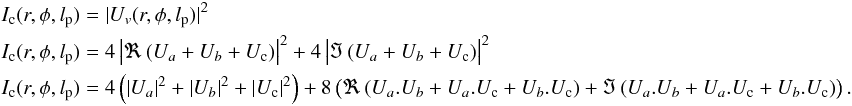 (M.1)The Lyot stop action is equivalent to a normalization of the radial Zernike polynomials with the diaphragm size dc < 1. This is a homothetic transformation in the ρ coordinate and
  ,
,  (M.2)The coronagraphic intensity consists of a linear part f(1) and a quadratic part f(2) as follows:
 ![Mathematical equation: \appendix \setcounter{section}{13} \begin{equation} \label{I2b} I_{\rm c}(r,\phi,l_{\rm p}) =4\left( \beta_N^0(d_{\rm c})\right)^2 \cdot \left|V_{N,0}^{l_{\rm p}} \right|^2+f^{(1)}\left[\beta_{\rm cn}^m(d_{\rm c}),\beta_{\rm sn}^m(d_{\rm c})\right]+f^{(2)}\left[(\beta_{\rm cn}^m(d_{\rm c}))^2,(\beta_{\rm sn}^m(d_{\rm c}))^2,(\beta_{\rm cn}^m(d_{\rm c})\cdot\beta_{\rm sn}^m(d_{\rm c}))\right] . \end{equation}](/articles/aa/full_html/2012/09/aa19614-12/aa19614-12-eq455.png) (M.3)Developing the squared terms yields
(M.3)Developing the squared terms yields ![Mathematical equation: \appendix \setcounter{section}{13} \begin{eqnarray} \label{I3} &&f^{(1)}\left[\beta_{\rm cn}^m(d_{\rm c}),\beta_{\rm sn}^m(d_{\rm c})\right]=\\ &&\qquad 8\: \sum_{n,m}^{\sim} \left[\left(\Re(\beta_N^0(d_{\rm c}))\Re(\beta_{\rm cn}^m(d_{\rm c}))+\Im(\beta_N^0(d_{\rm c}))\Im(\beta_{\rm cn}^m(d_{\rm c}))\right)\cdot \Re\left({\rm i}^m V_{n,m}^{l_{\rm p}} \: V_{N,0}^{l_{\rm p}*}\right)\:C_m(\phi)\right]\nonumber\\ &&\qquad -8\: \sum_{n,m}^{\sim} \left[\left(\Re(\beta_N^0(d_{\rm c}))\Im(\beta_{\rm cn}^m(d_{\rm c}))-\Im(\beta_N^0(d_{\rm c}))\Re(\beta_{\rm cn}^m(d_{\rm c}))\right)\cdot \Im\left({\rm i}^m V_{n,m}^{l_{\rm p}} \: V_{N,0}^{l_{\rm p}*}\right)\:C_m(\phi)\right]\nonumber\\ &&\qquad +8\: \sum_{n,m}^{\sim} \left[\left(\Re(\beta_N^0(d_{\rm c}))\Re(\beta_{\rm sn}^m(d_{\rm c}))+\Im(\beta_N^0(d_{\rm c}))\Im(\beta_{\rm sn}^m(d_{\rm c}))\right)\cdot \Re\left({\rm i}^m V_{n,m}^{l_{\rm p}} \: V_{N,0}^{l_{\rm p}*}\right)\:S_m(\phi)\right]\nonumber\\ &&\qquad -8\: \sum_{n,m}^{\sim} \left[\left(\Re(\beta_N^0(d_{\rm c}))\Im(\beta_{\rm sn}^m(d_{\rm c}))-\Im(\beta_N^0(d_{\rm c}))\Re(\beta_{\rm sn}^m(d_{\rm c}))\right)\cdot \Im\left({\rm i}^m V_{n,m}^{l_{\rm p}} \: V_{N,0}^{l_{\rm p}*}\right)\:S_m(\phi)\right]\nonumber \\ \label{I3b} && f^{(1)}\left[\beta_{\rm cn}^m(d_{\rm c}),\beta_{\rm sn}^m(d_{\rm c})\right]= \sum_{n,m}^{\sim}\left[\left(A_{\rm c}^m C_m(\phi) + A_{\rm s}^m S_m(\phi)\right) 8\Re\left({\rm i}^m V_{n,m}^{l_{\rm p}} \: V_{N,0}^{l_{\rm p}*}\right)\right] - \sum_{n,m}^{\sim}\left[\left(B_{\rm c}^m C_m(\phi) + B_{\rm s}^m S_m(\phi) \right) 8\Im\left({\rm i}^m V_{n,m}^{l_{\rm p}} \: V_{N,0}^{l_{\rm p}*}\right)\right] . ~~~~~~~~~~~~~ \end{eqnarray}](/articles/aa/full_html/2012/09/aa19614-12/aa19614-12-eq456.png) The
The  are defined as follows
 ![Mathematical equation: \appendix \setcounter{section}{13} \begin{eqnarray} \label{I3C} &&A_{\rm c}^m=\Re(\beta_N^0(d_{\rm c}))\Re(\beta_{\rm cn}^m(d_{\rm c}))+\Im(\beta_N^0(d_{\rm c}))\Im(\beta_{\rm cn}^m(d_{\rm c})) \qquad A_{\rm s}^m=\Re(\beta_N^0(d_{\rm c}))\Re(\beta_{\rm sn}^m(d_{\rm c}))+\Im(\beta_N^0(d_{\rm c}))\Im(\beta_{\rm sn}^m(d_{\rm c})) \\[1mm] && B_{\rm c}^m=\Re(\beta_N^0(d_{\rm c}))\Im(\beta_{\rm cn}^m(d_{\rm c}))-\Im(\beta_N^0(d_{\rm c}))\Re(\beta_{\rm cn}^m(d_{\rm c})) \qquad B_{\rm s}^m=\Re(\beta_N^0(d_{\rm c}))\Im(\beta_{\rm sn}^m(d_{\rm c}))-\Im(\beta_N^0(d_{\rm c}))\Re(\beta_{\rm sn}^m(d_{\rm c})) \\ &&f^{(2)}\left[(\beta_{\rm cn}^m(d_{\rm c}))^2,(\beta_{\rm sn}^m(d_{\rm c}))^2,(\beta_{\rm cn}^m(d_{\rm c})\cdot\beta_{\rm sn}^m(d_{\rm c}))\right] = \sum_{n,m}^{\sim}\left[ (-1)^m\left(\left(\beta_{\rm cn}^m(d_{\rm c})\right)^2 \:C^2_m(\phi) + \left(\beta_{\rm sn}^m(d_{\rm c})\right)^2\:S^2_m(\phi)\right)\cdot \left(V_{n,m}^{l_{\rm p}}\right)^2\right] \\ &&\hspace*{6.5cm}+ 8 \sum_{n,m}^{\sim}\left[\Re({\rm i}^m \beta_{\rm cn}^m(d_{\rm c}) \cdot \beta_{\rm sn}^m(d_{\rm c}))+\Im ({\rm i}^m \beta_{\rm cn}^m(d_{\rm c}) \cdot \beta_{\rm sn}^m(d_{\rm c}))\cdot \left(V_{n,m}^{l_{\rm p}}\right)^2 \:C_m(\phi)\:S_m(\phi)\right] . \nonumber \end{eqnarray}](/articles/aa/full_html/2012/09/aa19614-12/aa19614-12-eq458.png)
Appendix N: Derivation of 
We now define two sets of functions and :  (N.1)with ϵm = 1 for m = 0 and 2 in all other cases.
We have already defined the inner product: 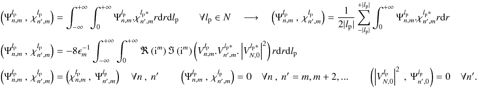 (N.2)The aberrated images are composed of several modes in sine and cosine functions. The first step of the image analysis is the decoupling of these modes, which can be performed with a polar Fourier transform Fp of the coronagraphic images. It is given by
  (N.3)In the perfect case without photon and readout noise, the Nijboer-Zernike analysis shows that
  .
.
For a linear approximation of the final coronagraphic intensity, ![Mathematical equation: \appendix \setcounter{section}{14} \begin{equation} \Psi_{\rm meas}^{m}(r,l_{\rm p})\approx\frac{1}{2\pi} \int_0^{2\pi} \left(4\left( \beta_N^0(d_{\rm c})\right)^2 \cdot \left|V_{N,0}^{l_{\rm p}} \right|^2+f^{(1)}\left[\beta_n^m(d_{\rm c})\right] \right) {\rm e}^{{\rm i} m\phi} {\rm d}\phi . \end{equation}](/articles/aa/full_html/2012/09/aa19614-12/aa19614-12-eq466.png) (N.4)Now, we can write the polar Fourier transform of the the final coronagraphic images using the Ψ,χ functions.
(N.4)Now, we can write the polar Fourier transform of the the final coronagraphic images using the Ψ,χ functions. ![Mathematical equation: \appendix \setcounter{section}{14} \begin{eqnarray} \label{f2} &&F_{\rm p}\left(4\left( \beta_N^0(d_{\rm c})\right)^2 \cdot \left|V_{N,0}^{l_{\rm p}} \right|^2\right) = \frac{1} {2} \left( \beta_N^0(d_{\rm c})\right)^2 \chi_{N,0}^{l_{\rm p}}\\[1.5mm] && F_{\rm p}\left(C_m(\phi)\right) = 1 \quad (m=0) \qquad F_{\rm p}\left(C_m(\phi)\right) = 1/2 \quad (0<m\leq n)\\[1.5mm] && F_{\rm p}\left(S_m(\phi)\right) = 0 \quad (m=0) \qquad F_{\rm p}\left(S_m(\phi)\right) = i/2 \quad (0<m\leq n)~~~~~~~~~~~ \end{eqnarray}](/articles/aa/full_html/2012/09/aa19614-12/aa19614-12-eq468.png) – m = 0
– m = 0 ![Mathematical equation: \appendix \setcounter{section}{14} \begin{eqnarray} \label{f3} \Psi_{\rm meas}^{0}\approx\frac{1} {2} \left( \beta_N^0(d_{\rm c})\right)^2 \chi_{N,0}^{l_{\rm p}}&&+ \sum_{n}^{\sim} A_{\rm c}^0(n) \chi_{n,0}^{l_{\rm p}} + \sum_{n}^{\sim} B_{\rm c}^0(n) \Psi_{n,0}^{l_{\rm p}}\nonumber \\ \Psi_{\rm meas}^{0}\approx\frac{1} {2} \left( \beta_N^0(d_{\rm c})\right)^2 \chi_{N,0}^{l_{\rm p}}&&+ \sum_{n}^{\sim}\left( \left[\left(\Re(\beta_N^0(d_{\rm c}))\Re(\beta_{\rm cn}^0(d_{\rm c}))+\Im(\beta_N^0(d_{\rm c}))\Im(\beta_{\rm cn}^0(d_{\rm c}))\right)\right]\cdot \chi_{n,0}^{l_{\rm p}}\right) \nonumber \\ &&+\sum_{n}^{\sim}\left(\left[\left(\Re(\beta_N^0(d_{\rm c}))\Im(\beta_{\rm cn}^0(d_{\rm c}))-\Im(\beta_N^0(d_{\rm c}))\Re(\beta_{\rm cn}^0(d_{\rm c}))\right)\right]\cdot \Psi_{n,0}^{l_{\rm p}}\right) \end{eqnarray}](/articles/aa/full_html/2012/09/aa19614-12/aa19614-12-eq469.png) (N.8)– 0 < m < n
(N.8)– 0 < m < n![Mathematical equation: \appendix \setcounter{section}{14} \begin{eqnarray} \label{f4} \Psi_{\rm meas}^{m}\; &&\approx \sum_{n}A^m_{\rm c}(n) \chi_{n,m}^{l_{\rm p}} +\sum_{n}B^m_{\rm c}(n) \Psi_{n,m}^{l_{\rm p}} + {\rm i}\sum_{n}A^m_{\rm s}(n) \chi_{n,m}^{l_{\rm p}} + {\rm i}\sum_{n}B^m_{\rm s}(n) \Psi_{n,m}^{l_{\rm p}}\nonumber \\ \Psi_{\rm meas}^{m}\; &&\approx\sum_{n} \left[\left(\Re(\beta_N^0(d_{\rm c}))\Re(\beta_{\rm cn}^m(d_{\rm c}))+\Im(\beta_N^0(d_{\rm c}))\Im(\beta_{\rm cn}^m(d_{\rm c}))\right)\right]\cdot \chi_{n,m}^{l_{\rm p}} \nonumber \\ &&+\sum_{n}\left[\left(\Re(\beta_N^0(d_{\rm c}))\Im(\beta_{\rm cn}^m(d_{\rm c}))-\Im(\beta_N^0(d_{\rm c}))\Re(\beta_{\rm cn}^m(d_{\rm c}))\right)\right]\cdot \Psi_{n,m}^{l_{\rm p}}\nonumber\\ &&+{\rm i}\sum_{n} \left[\left(\Re(\beta_N^0(d_{\rm c}))\Re(\beta_{\rm sn}^m(d_{\rm c}))+\Im(\beta_N^0(d_{\rm c}))\Im(\beta_{\rm sn}^m(d_{\rm c}))\right))\right]\cdot \chi_{n,m}^{l_{\rm p}}\nonumber\\ &&+{\rm i}\sum_{n}\left[\left(\Re(\beta_N^0(d_{\rm c}))\Im(\beta_{\rm sn}^m(d_{\rm c}))-\Im(\beta_N^0(d_{\rm c}))\Re(\beta_{\rm sn}^m(d_{\rm c}))\right)\right]\cdot \Psi_{n,m}^{l_{\rm p}} \end{eqnarray}](/articles/aa/full_html/2012/09/aa19614-12/aa19614-12-eq470.png) (N.9)– m = n
(N.9)– m = n![Mathematical equation: \appendix \setcounter{section}{14} \begin{eqnarray} \label{f5} \Psi_{\rm meas}^{n}\; &&\approx \sum_{n}A_{\rm c}^n(n) \chi_{n,n}^{l_{\rm p}} +\sum_{n}B_{\rm c}^n(n) \Psi_{n,n}^{l_{\rm p}}-{\rm i}\: {\rm Sign}(l_{\rm p}) \sum_{n}A_{\rm s}^n(n) \chi_{n,n}^{l_{\rm p}} -{\rm i}\: {\rm Sign}(l_{\rm p})\sum_{n}B_{\rm s}^n(n) \Psi_{n,n}^{l_{\rm p}} \nonumber \\[1mm] &&\quad +\sum_{n}A_{\rm s}^n(n) \chi_{n,n}^{l_{\rm p}} +\sum_{n}B_{\rm s}^n(n) \Psi_{n,n}^{l_{\rm p}}+{\rm i}\: {\rm Sign} (l_{\rm p}) \sum_{n}A_{\rm c}^n(n) \chi_{n,n}^{l_{\rm p}} +{\rm i}\: {\rm Sign}(l_{\rm p})\sum_{n}B_{\rm c}^n(n) \Psi_{n,n}^{l_{\rm p}}\nonumber \\[1mm] \Psi_{\rm meas}^{n}\; &&\approx\sum_{n}\left[\left(\Re(\beta_N^0(d_{\rm c}))\Re(\beta_{\rm cn}^n(d_{\rm c}))+\Im(\beta_N^0(d_{\rm c}))\Im(\beta_{\rm cn}^n(d_{\rm c}))\right)\right]\cdot \chi_{n,n}^{l_{\rm p}} \nonumber \\[1mm] &&+\sum_{n}\left[\left(\Re(\beta_N^0(d_{\rm c}))\Im(\beta_{\rm cn}^n(d_{\rm c}))-\Im(\beta_N^0(d_{\rm c}))\Re(\beta_{\rm cn}^n(d_{\rm c}))\right)\right]\cdot \Psi_{n,n}^{l_{\rm p}}\nonumber\\[1mm] &&+\sum_{n} \left[\left(\Re(\beta_N^0(d_{\rm c}))\Re(\beta_{\rm sn}^n(d_{\rm c}))+\Im(\beta_N^0(d_{\rm c}))\Im(\beta_{\rm sn}^n(d_{\rm c}))\right))\right]\cdot \chi_{n,n}^{l_{\rm p}}\nonumber\\[1mm] &&+\sum_{n}\left[\left(\Re(\beta_N^0(d_{\rm c}))\Im(\beta_{\rm sn}^n(d_{\rm c}))-\Im(\beta_N^0(d_{\rm c}))\Re(\beta_{\rm sn}^n(d_{\rm c}))\right)\right]\cdot \Psi_{n,n}^{l_{\rm p}}\nonumber\\[1mm] &&-{\rm i}\: {\rm Sign}(l_{\rm p})\sum_{n}\left[\left(\Re(\beta_N^0(d_{\rm c}))\Re(\beta_{\rm cn}^n(d_{\rm c}))+\Im(\beta_N^0(d_{\rm c}))\Im(\beta_{\rm cn}^n(d_{\rm c}))\right)\right]\cdot \chi_{n,n}^{l_{\rm p}} \nonumber \\[1mm] &&-{\rm i}\: {\rm Sign}(l_{\rm p})\sum_{n}\left[\left(\Re(\beta_N^0(d_{\rm c}))\Im(\beta_{\rm cn}^n(d_{\rm c}))-\Im(\beta_N^0(d_{\rm c}))\Re(\beta_{\rm cn}^n(d_{\rm c}))\right)\right]\cdot \Psi_{n,n}^{l_{\rm p}}\nonumber\\[1mm] &&+{\rm i}\: {\rm Sign}(l_{\rm p})\sum_{n} \left[\left(\Re(\beta_N^0(d_{\rm c}))\Re(\beta_{\rm sn}^n(d_{\rm c}))+\Im(\beta_N^0(d_{\rm c}))\Im(\beta_{\rm sn}^n(d_{\rm c}))\right))\right]\cdot \chi_{n,n}^{l_{\rm p}}\nonumber\\[1mm] &&+{\rm i}\: {\rm Sign}(l_{\rm p})\sum_{n}\left[\left(\Re(\beta_N^0(d_{\rm c}))\Im(\beta_{\rm sn}^n(d_{\rm c}))-\Im(\beta_N^0(d_{\rm c}))\Re(\beta_{\rm sn}^n(d_{\rm c}))\right)\right]\cdot \Psi_{n,n}^{l_{\rm p}}. \end{eqnarray}](/articles/aa/full_html/2012/09/aa19614-12/aa19614-12-eq471.png) (N.10)Using the inner products between the
(N.10)Using the inner products between the  and the
  functions, it is now possible to retrieve coefficients of the linear system of equation as follows: – m = 0
 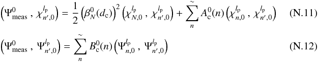 – 0 < m < n
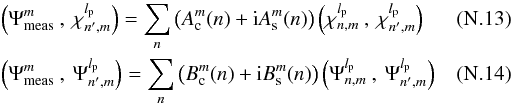 – m = n
![Mathematical equation: \appendix \setcounter{section}{14} \begin{eqnarray} \label{f6c} &&\left(\Psi_{\rm meas}^{n},\:\chi_{n',n}^{l_{\rm p}}\right)=\sum_{n} \left(\left[A^n_{\rm c}(n)+A^n_{\rm s}(n)\right]+{\rm i}\: {\rm Sign}(l_{\rm p})\left[A^n_{\rm c}(n)-A^n_{\rm s}(n)\right] \right) \left(\chi_{n,n}^{l_{\rm p}}\:,\:\chi_{n',n}^{l_{\rm p}}\right)\\[1mm] &&\left(\Psi_{\rm meas}^{n},\:\Psi_{n',n}^{l_{\rm p}}\right)=\sum_{n} \left(\left[B^n_{\rm c}(n)+B^n_{\rm s}(n)\right]+{\rm i}\: {\rm Sign}(l_{\rm p})\left[B^n_{\rm c}(n)-B^n_{\rm s}(n)\right] \right) \left(\Psi_{n,n}^{l_{\rm p}}\:,\: \Psi_{n',n}^{l_{\rm p}}\right) \\[1mm] \label{lse1bis} && G.u\left[\beta_n^m\right]=r \qquad \quad u\left[\beta_n^0\right] = [A_{\rm c}^0(n), B_{\rm c}^0(n)] \qquad u\left[\beta_n^m\right]=[A^m_{\rm c}(n), A^m_{\rm s}(n), B^m_{\rm c}(n), B^m_{\rm s}(n)],\qquad u\left[\beta_n^n\right]=[A^n_{\rm c}(n), A^n_{\rm s}(n), B^n_{\rm c}(n), B^n_{\rm s}(n)]\nonumber\\[1mm] && G_{n,n'}^{m,l_{\rm p}} \left(\Psi\right) = \left(\Psi_{n,m}^{l_{\rm p}}\:,\:\Psi_{n',m}^{l_{\rm p}}\right) \qquad G_{n,n'}^{m,l_{\rm p}} \left(\chi\right) = \left(\chi_{n,m}^{l_{\rm p}}\:,\:\chi_{n',m}^{l_{\rm p}}\right) \\[1mm] \label{lse2bis1} &&r_{n'}^{0,l_{\rm p}}\left(\Psi\right) = \left(\Psi_{\rm meas}^{0}\:,\:\Psi_{n',0}^{l_{\rm p}}\right) \qquad r_{n'}^{0,l_{\rm p}}\left(\chi\right) = \left(\Psi_{\rm meas}^{0}\:,\:\chi_{n',0}^{l_{\rm p}}\right) \quad (m=0)\nonumber \\[1mm] &&r_{n'}^{m,l_{\rm p}}\left(\Psi\right) = \left(\Psi_{\rm meas}^{m}\:,\:\Psi_{n',m}^{l_{\rm p}}\right) \qquad r_{n'}^{m,l_{\rm p}}\left(\chi\right) = \left(\Psi_{\rm meas}^{m}\:,\:\chi_{n',m}^{l_{\rm p}}\right) \quad (0<m<n)\nonumber\\[1mm] &&r_{n'}^{n,l_{\rm p}}\left(\Psi\right) = \left(\Psi_{\rm meas}^{n}\:,\:\Psi_{n',n}^{l_{\rm p}}\right) \qquad r_{n'}^{n,l_{\rm p}}\left(\chi\right) = \left(\Psi_{\rm meas}^{n}\:,\:\chi_{n',n}^{l_{\rm p}}\right) \quad (m=n) \: .\nonumber \end{eqnarray}](/articles/aa/full_html/2012/09/aa19614-12/aa19614-12-eq476.png)
Appendix O: Scattering function
The physical theory of scattering by small particles is the Mie theory (Bohren & Huffman 1983), but this mathematical development is too complicated to be used with spherical Bessel and infinite sum of Legendre polynomials. The Henyey-Greenstein model (Henyey & Greenstein 1941) is a useful approximation to describe the angular distribution of light scattered by small particles. At the beginning, this model was applied to scattering by interstellar dust clouds in the Milky-Way. It is now used in numerous situations, ranging from the scattering of light in biological tissues to scattering caused by bulk material in an optical system.
In this model, the angular distribution of scattered light is given by ![Mathematical equation: \appendix \setcounter{section}{15} \begin{equation} \label{scat1} S{\rm c}(\theta)=\frac{1} {4\pi} \frac{1-g^2} {\left[1+g^2-2g.\cos(\theta)\right]^{3/2}} \quad \int_0^{2\pi}\int_0^{\pi} S{\rm c}(\theta) \sin(\theta) {\rm d}\theta {\rm d}\phi=1 .\nonumber \end{equation}](/articles/aa/full_html/2012/09/aa19614-12/aa19614-12-eq477.png) The Henyey-Greenstein phase function Sc(θ) is governed by the variation of only one parameter, , and ranges from backscattering through isotropic scattering to forward scattering. The θ and φ variables are the classical angular coordinates. Forward scattering is θ = 0, while for back-scattering, θ = π. We see that the ratio of forward-to-back scattering is [(1 + g)/(1 − g)] 3.
The Henyey-Greenstein phase function Sc(θ) is governed by the variation of only one parameter, , and ranges from backscattering through isotropic scattering to forward scattering. The θ and φ variables are the classical angular coordinates. Forward scattering is θ = 0, while for back-scattering, θ = π. We see that the ratio of forward-to-back scattering is [(1 + g)/(1 − g)] 3.
For g > 0, forward scattering is dominant, while for g < 0, backscattering predominates. To use the H-G function for Monte Carlo models, we need the accumulated distribution: ![Mathematical equation: \appendix \setcounter{section}{15} \begin{eqnarray} \label{scat2} &&P(\cos(\theta))=\int_{-1}^{\cos(\theta)} \frac{(1-g^2) {\rm d}(\cos(\theta))}{\left[1+g^2-2g.\cos(\theta)\right]^{3/2}}\\ &&P(\cos(\theta))=\frac{1-g^2}{2g} \left( \left(1+g^2-2g.\cos(\theta)\right)^{-1/2}-(1+g)^{-1}\right) \qquad \cos(\theta)=\frac{1}{2g} \left(1+g^2-\left( \frac{1-g^2} {1+g(2P-1)}\right)^2 \right)\cdot \nonumber \end{eqnarray}](/articles/aa/full_html/2012/09/aa19614-12/aa19614-12-eq485.png) (O.1)The Zemax software uses this approximation for scattering calculation, and we obtain
(O.1)The Zemax software uses this approximation for scattering calculation, and we obtain
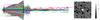 |
Fig. O.1 Non-sequential Zemax analysis of the proposed optical implementation after the Lyot stop to split the two circular polarizations. Left: the polychromatic ray tracing (650–900 nm) for one polarization, and right: the detector view of no-coherent intensity distribution in logarithmic scale. With these classical materials (MgF2, quartz, infrasil) the maximum scattered light is 10-6 of the residual coronagraphic intensity. In this simulation, we chose an anti-reflexion coating of 0.5% per surface. |
Appendix P: Polychromatic simulations and speckles smearing
We present in this section a complete set of numerical simulations obtained in wide bandpass with an imperfect vortex phase-mask. The inputs of these simulations were given in Sect. 7.2:
-
The input Strehl ratio is 95% @ 650 nm with the first 860 Zernikes (40 complete modes).
-
An imperfect phase-mask: where the s-transmittance is 97%, the p-transmittance is 98% and the local phase retardance is π ± Δφ with a quadratic law for the phase error of the mask.
-
Common and non-common path error are λ/71 rms @ 650 nm (the total is λ/50 rms at 650 nm).
-
Polishing error: DSP f-2 with a shift of 8.1% for non-common path error.
-
Polychromatic speckle smearing due to residual Wollaston chromatism given by the Zemax model.
-
Photon noise, readout noise (6 e − ), full-well capacity of 105e − , residual flat of 1% rms.
P.1. Telescope pupil and coronagraphic pupil phase screens
We present the entrance pupil for a perfect circular telescope (off-axis configuration) obtained by the direct summation of the first 860 Zernikes, and also the two phase-screens using a density spectral power function (f-2) where f is the spatial frequency in the Fourier domain.
 |
Fig. P.1 Left to right: the telescope entrance pupil phase obtained with the first 40 Zernike modes. The Strehl ratio is 95% @ 650 nm. In the center, the phase screen that simulates high-frequency polishing defaults for the lp = 2 beam. Right, the phase screen for the lp = −2 beam. These two last phase screens are the superposition of two different random simulations (common and non-common path errors). The last case (lp = −2) is simulated with a shift of the second phase screen (8.1% in the y-axis with respect to the pupil diameter). The sigma of the two phase error screens for lp = 2 and lp = −2 are chosen equal to λ/50 rms @ 650 nm. |
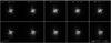 |
Fig. P.2 Set of numerical coronagraphic simulations with a maximum phase-shift (Δφmax) on the vortex mask of 0.001 radian for each bandpass. We chose five different bandpasses: Δλ = 2 nm (corresponding to a single-mode Laser diode), 100 nm, 150 nm (R-filter), 200 nm, and finally 250 nm (R to I astronomical filters). These simulations show the anti-symmetric smearing (bottom: lp = −2, top: lp = 2 images) due to the Wollaston optical component and also a high-contrast in the residual speckle due to the wavelength filtering by the coronagraphic device. Indeed, only wavelengths with larger phase-shift errors on the phase-mask (λmax,λmin) have a significant effect on the final coronagraphic images. We recall that for λmax the effect is less than λmin due to a better Strehl ratio. |
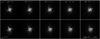 |
Fig. P.3 Same coronagraphic simulations with a maximum phase-shift of 0.01 radian. |
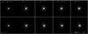 |
Fig. P.4 Same coronagraphic simulations with a maximum phase-shift of 0.1 radian. A coronagraphic strong peak residual appears in the center of the image (β0,0 ≠ 0). |
P.2. Phase error on the vortex coronagraph
The π phase-shift of the vortex coronagraph is generally obtained by index material engineering as engraving a ramp in a material for scalar vortex or in liquid crystal polymer (LCP) using birefringent optical properties, see Mawet et al. (2009) to generate the proper phase helix. The refractive index of the material as a function of the wavelength follows a Sellmeiler law (λ2) (also for the LCP material). This property generates a π phase-shift with a quadratic dependance. In these conditions, the phase-shift error increases strongly at the edges of the chosen wavelength bandpass. To perform our numerical simulations, we chose the following phase-shift wavelength dependence:  (P.1)where Δφmax is the maximum phase-shift error in radian (0.001,0.01,0.1), λ0 is the centering mask wavelength (where the phase-shift is π) and finally λmax,λmin corresponds to the wavelength bandpass edges.
P.3. Wollaston residual dispersion
Our optical implementation presents an artificial polychromatic speckle smearing in the x-axis due to the Wollaston residual dispersion. If we use the Sellmeiler law for the refractive index of the MgF2 or the position of the spot diagram in the Zemax software, we can know the shift of the PSF as a function of the wavelength on the two coronagraphic images. The position of the PSF center in λ/d units is given with very good approximation ± 0.2 μm by the following function:  (P.2)The position of the PSF is completely anti-symmetric in the ± 0.01λ/d level with respect to the sign of the vortex charge lp.
P.4. Coronagraphic vortex numerical simulations set
The Fourier simulation was performed on 2K × 2K arrays with an entrance perfect circular pupil of 255 pixels diameter. The chromatism was taken into account by changing the diameter of the entrance pupil with one pixel steps that correspond to ≈ 7 nm bandpass steps. For the smaller bandpass (2 nm – the Laser diode), the simulation was performed with 4K × 4K arrays and a circular pupil of 511 pixels diameter. The entrance pupil phase was scaled and a vortex coronagraphic mask was created for each wavelength with the proper s and p transmittance and the mask phase-shift error. The diaphragm was chosen to be just smaller the pupil diameter (98%, 2 pixels apart) and scaled with respect the wavelength. We chose this non-optimized configuration (see Appendix K) to use the βn,m coefficients without a scaling factor. A phase screen error was added to each coronagraphic pupil (lp = ± 2) to take the common on the non-common path error of the optical train (Wollaston and achromatic doublet) into account. This phase screen includes the shift of the two beams due to the polarization separation (non-common path error). The maximum shift between the two beams is 8.1% at the output of the final imaging lens doublet, this is the value adopted in our Fourier numerical simulations. Finally, we used Eq. (P.2) to produce the Wollaston chromatic smearing in the coronagraphic image plane by adding a tip in the coronagraphic pupil. These simulations complete the previous results presented in Sect. 7.2, and we show here some images obtained for three maximum phase-shift errors of Δφmax = 0.001,0.01,0.1 radian and five different wavelength bandpasses Δλ = 2,100,150,200,250 nm, also including photon noise with 80 000 e − on the maximum of coronagraphic image (80% of the full-well capacity), readout noise (6e − ), and flat noise (1% rms).
Appendix Q: FFT vs. NZ for a “sin” ripple case
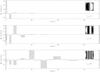 |
Fig. Q.1
|
We present in this appendix a complete set of numerical simulations obtained for a perfect case with a simple “sin” function in the entrance pupil plane. A sin modulation is proposed for both phase and amplitude. The pupil becomes ![Mathematical equation: \appendix \setcounter{section}{17} \begin{equation} \label{sinx} \Pi=\Pi(0,1) \left[1 - A_a/2 + A_a \sin(2\pi f_x x)/2+ {\rm i} A_{\Phi} \sin(2\pi f_x x)/2 \right] \qquad A_{\Phi}=0.1\lambda_0 \quad A_a=0.01 \quad f_x=2,4,8 \quad \lambda_0=650~{\rm nm}, \end{equation}](/articles/aa/full_html/2012/09/aa19614-12/aa19614-12-eq514.png) (Q.1)where AΦ, Aa are the coefficients of the phase and amplitude errors applied in the pupil respectively, and fx is the spatial frequency of the sin function. The direct decomposition of the three sin modulations is presented in the following figure: the modal decomposition is not well-suited for a “simple” sin function as wavefront error. Indeed, the term “simple” can be applied for the classical Fourier transform in cartesian coordinates (only one frequency in the Fourier plane), but not in the Zernike polynomials basis, where it is necessary to use many coefficients. We propose to compare the FFT propagation with VVC and the NZ modal decomposition for these three spatial frequencies.
(Q.1)where AΦ, Aa are the coefficients of the phase and amplitude errors applied in the pupil respectively, and fx is the spatial frequency of the sin function. The direct decomposition of the three sin modulations is presented in the following figure: the modal decomposition is not well-suited for a “simple” sin function as wavefront error. Indeed, the term “simple” can be applied for the classical Fourier transform in cartesian coordinates (only one frequency in the Fourier plane), but not in the Zernike polynomials basis, where it is necessary to use many coefficients. We propose to compare the FFT propagation with VVC and the NZ modal decomposition for these three spatial frequencies.
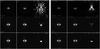 |
Fig. Q.2 Set of numerical monochromatic coronagraphic simulations with a vortex mask error of 0.001 radian. The input sin frequency is chosen as fx = 2 (low-order wavefront error). Each graphic is organized as follows: Left to right: lp = + 2 coronagraphic image, lp = −2 coronagraphic image, difference between the two previous images with an amplification of intensity level of 100. Upper: pure amplitude wavefront error (Aa = 0.01), middle: pure phase error (AΦ = 0.1λ0), and bottom: both errors, amplitude and phase. The first nine sets of figures left is for the FFT propagation, whereas the nine sets of figures right is for direct |
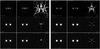 |
Fig. Q.3 Two sets of numerical simulations FFT vs. NZ with a sinus frequency of fx = 4. |
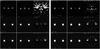 |
Fig. Q.4 Two sets of numerical simulations FFT vs. NZ with a sinus frequency of fx = 8 (high-order wavefront error). |
All Tables
Maximum coronagraphic nulling ratio and wavelength bandpass achievable for various levels of input Strehl ratio.
All Figures
|
Fig. 1 Schematic view of the NZ vortex phase-retrieval process. It consists of using the real input coronagraphic images, corresponding to lp = 0, ± 2 (the lp = ± 2 images are provided by polarization splitting, while the unpolarized image (lp = 0) is directly given by the sum of the two polarized images) projected on aberrations templates, and finding the unknown coefficients by resolving a system of linear equations. Left: the three images needed for the full aberration analysis. Center: linear systems to retrieve the |
| In the text | |
|
Fig. 2 Polarization splitter analysis: possible implementation of the polarization splitter system used after the Lyot stop. An achromatic quarter-wave plate (quartz/MgF2) and a Wollaston in MgF2 combined here with a simple achromatic doublet. This simple optical implementation allows us to image the two residual coronagraphic images in the left and right circular polarization basis on the detector. The two images presented in this figure in logarithmic gray scale show the two polychromatic PSF (650–900 nm) obtained by this simple scheme for the two circular polarization images. Note that the PSF shows a small chromatic smearing residual on the x-axis (Strehl = 96.5%) due to the substantial wavelength bandpass. This polychromatic smearing is detailed in Appendix P. |
| In the text | |
|
Fig. 3 Numerical simulation illustrating the principle of Nijboer-Zernike retrieval applied on the vortex coronagraph. (Up to down), numerical simulation for each circular polarization with lp = 2 and lp = −2 respectively using the first 860 Zernike polynomials (40 complete modes) and a Lyot stop of 99%. The Strehl ratio of the PSF before coronagraphic filtering is 95%. The Lyot stop remove the strong diffraction value in ρ = 1 but allows us to show all images without scaling the |
| In the text | |
|
Fig. 4 Polychromatic coronagraphic simulation for lp = 2 with Δλ = 250 nm of spectral bandpass and a phase error of Δφ = ± 0.001 radian for the vortex mask. We also include defects of our optical implementation. Left: without the speckle smearing. Right: with the Wollaston speckle smearing. The chromatic effect on the speckles is small in the two cases, the contrast remains high. The brightness scale is the same between the two images and is not linear. |
| In the text | |
|
Fig. 5
|
| In the text | |
|
Fig. 6
|
| In the text | |
|
Fig. D.1 Input classical Zernike |
| In the text | |
|
Fig. D.2
|
| In the text | |
|
Fig. D.3
|
| In the text | |
|
Fig. D.4 Uv(r,φ),lp = ± 2 functions in the coronagraphic image plane for the 10 Zernike polynomials (Z2 − Z11). Top: lp = + 2, Bottom: lp = −2. The vertical solid line separates the real part from the imaginary part of the two Uv(r,φ) functions. |
| In the text | |
|
Fig. G.1 Comparison between Fourier simulations for each Zernike polynomial (2-860) and |
| In the text | |
|
Fig. G.2 Comparison between Fourier simulations for each Zernike polynomial (2-860) and |
| In the text | |
|
Fig. H.1
|
| In the text | |
|
Fig. H.2
|
| In the text | |
|
Fig. K.1 Variation of the residual energy (dEp/dx) in the residual optical aberrations as a function of the number of Zernike polynomials used (nz – without the piston term) and the power spectral density 1/npw. The figure shows two diaphragm values: when the gain is maximum and when it is equal to zero. The figure in 1/n presents strong residual oscillations owing to low-order aberrations. |
| In the text | |
|
Fig. K.2 Fresnel diffraction of the Lyot stop with an optical vortex coronagraph. We present the real and the imaginary parts of the |
| In the text | |
|
Fig. L.1 Spider Fresnel diffraction calculation for a VLT coronagraphic pupil (ϵ = 0.14) and the diameter of the coronagraphic pupil of 18 mm. The figure shows a comparison between the classical Fresnel diffraction (lp = 0) and the optical propagation including the vortex (lp = 2). The thickness of the spider is 225 μm. |
| In the text | |
|
Fig. O.1 Non-sequential Zemax analysis of the proposed optical implementation after the Lyot stop to split the two circular polarizations. Left: the polychromatic ray tracing (650–900 nm) for one polarization, and right: the detector view of no-coherent intensity distribution in logarithmic scale. With these classical materials (MgF2, quartz, infrasil) the maximum scattered light is 10-6 of the residual coronagraphic intensity. In this simulation, we chose an anti-reflexion coating of 0.5% per surface. |
| In the text | |
|
Fig. P.1 Left to right: the telescope entrance pupil phase obtained with the first 40 Zernike modes. The Strehl ratio is 95% @ 650 nm. In the center, the phase screen that simulates high-frequency polishing defaults for the lp = 2 beam. Right, the phase screen for the lp = −2 beam. These two last phase screens are the superposition of two different random simulations (common and non-common path errors). The last case (lp = −2) is simulated with a shift of the second phase screen (8.1% in the y-axis with respect to the pupil diameter). The sigma of the two phase error screens for lp = 2 and lp = −2 are chosen equal to λ/50 rms @ 650 nm. |
| In the text | |
|
Fig. P.2 Set of numerical coronagraphic simulations with a maximum phase-shift (Δφmax) on the vortex mask of 0.001 radian for each bandpass. We chose five different bandpasses: Δλ = 2 nm (corresponding to a single-mode Laser diode), 100 nm, 150 nm (R-filter), 200 nm, and finally 250 nm (R to I astronomical filters). These simulations show the anti-symmetric smearing (bottom: lp = −2, top: lp = 2 images) due to the Wollaston optical component and also a high-contrast in the residual speckle due to the wavelength filtering by the coronagraphic device. Indeed, only wavelengths with larger phase-shift errors on the phase-mask (λmax,λmin) have a significant effect on the final coronagraphic images. We recall that for λmax the effect is less than λmin due to a better Strehl ratio. |
| In the text | |
|
Fig. P.3 Same coronagraphic simulations with a maximum phase-shift of 0.01 radian. |
| In the text | |
|
Fig. P.4 Same coronagraphic simulations with a maximum phase-shift of 0.1 radian. A coronagraphic strong peak residual appears in the center of the image (β0,0 ≠ 0). |
| In the text | |
|
Fig. Q.1
|
| In the text | |
|
Fig. Q.2 Set of numerical monochromatic coronagraphic simulations with a vortex mask error of 0.001 radian. The input sin frequency is chosen as fx = 2 (low-order wavefront error). Each graphic is organized as follows: Left to right: lp = + 2 coronagraphic image, lp = −2 coronagraphic image, difference between the two previous images with an amplification of intensity level of 100. Upper: pure amplitude wavefront error (Aa = 0.01), middle: pure phase error (AΦ = 0.1λ0), and bottom: both errors, amplitude and phase. The first nine sets of figures left is for the FFT propagation, whereas the nine sets of figures right is for direct |
| In the text | |
|
Fig. Q.3 Two sets of numerical simulations FFT vs. NZ with a sinus frequency of fx = 4. |
| In the text | |
|
Fig. Q.4 Two sets of numerical simulations FFT vs. NZ with a sinus frequency of fx = 8 (high-order wavefront error). |
| In the text | |
Current usage metrics show cumulative count of Article Views (full-text article views including HTML views, PDF and ePub downloads, according to the available data) and Abstracts Views on Vision4Press platform.
Data correspond to usage on the plateform after 2015. The current usage metrics is available 48-96 hours after online publication and is updated daily on week days.
Initial download of the metrics may take a while.