| Issue |
A&A
Volume 553, May 2013
|
|
|---|---|---|
| Article Number | A32 | |
| Number of page(s) | 9 | |
| Section | Galactic structure, stellar clusters and populations | |
| DOI | https://doi.org/10.1051/0004-6361/201220937 | |
| Published online | 25 April 2013 | |
Crucial aspects of the initial mass function
II. The inference of total quantities from partial information on a cluster
1
Instituto de Astrofísica de Andalucía (IAA-CSIC),
Glorieta de la Astronomía s/n,
18008
Granada,
Spain
e-mail: This email address is being protected from spambots. You need JavaScript enabled to view it.
2
Instituto de Astrofísica de Canarias, c/vía Láctea s/n, 38205
La Laguna, Tenerife,
Spain
3
Instituto de Astronomía, Universidad Académica en Ensenada,
Universidad Nacional Autónoma de México, Ensenada BC, 22860
Mexico,
Mexico
4
European Southern Observatory, Casilla 19001, Santiago 19, Chile
5
Max Planck Institut für Astronomie, Königstuhl 17, 69117
Heidelberg,
Germany
6
Departamento de Astrofísica, Universidad de La Laguna
(ULL), 38205, La
Laguna, Tenerife,
Spain
7
S. D. Astronomía y Geodesia, Fac. CC. Matemáticas, Universidad
Complutense de Madrid, 28040
Madrid,
Spain
Received:
17
December
2012
Accepted:
21
February
2013
Abstract
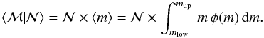
Context. In a probabilistic framework of the interpretation of the initial mass function (IMF), the IMF cannot be arbitrarily normalized to the total mass, ℳ, or number of stars, N, of the system. Hence, the inference of ℳ and N when partial information about the studied system is available must be revised (i.e., the contribution to the total quantity cannot be obtained by simple algebraic manipulations of the IMF).
Aims. We study how to include constraints in the IMF to make inferences about different quantities characterizing stellar systems. It is expected that including any particular piece of information about a system would constrain the range of possible solutions. However, different pieces of information might be irrelevant depending on the quantity to be inferred. In this work we want to characterize the relevance of the priors in the possible inferences.
Methods. Assuming that the IMF is a probability distribution function, we derive the sampling distributions of ℳ and N of the system constrained to different types of information available.
Results. We show that the value of ℳ that would be inferred must be described as a probability distribution Φℳ[ℳ;ma,Na,ΦN(N)] that depends on the completeness limit of the data, ma, the number of stars observed down to this limit, Na, and the prior hypothesis made on the distribution of the total number of stars in clusters, ΦN(N).
Key words: stars: statistics / galaxies: stellar content / methods: data analysis
© ESO, 2013
1. Introduction
The study of cluster dynamics and star formation relies on the knowledge of cluster masses and the amount of such mass transformed into stars, ℳ. In most cases, we have partial information of the system, i.e., the observations of some stars in the cluster. Such information is usually used in the inverse problem using the initial mass function (IMF) realization (see below) as a distribution by number to make inferences about a theoretical probability distribution function, the IMF φ(m) (Bouvier et al. 1998; Briceño et al. 2002; Luhman et al. 2003; Oliveira et al. 2009; Bayo et al. 2011). However, such information is not enough to obtain cluster masses, and for some astrophysical studies it is required to assume a φ(m) covering all the range of possible stellar masses to make inferences about global cluster properties (the direct problem).
This use of the term IMF for both the distribution by number for the inverse problem of statistics and the probability distribution function (PDF) for the direct problem can lead to different interpretations of the IMF itself and the results obtained from it (cf. Cerviño et al. 2013,hereafter Paper I). In this work, following Scalo (1986), we will adopt the PDF definition1.
The shape of the PDF and that of the distribution by number depend crucially on the size of
the sample, that is, the number of stars  ;
for large
values, the two shapes tend to be similar. However, this similarity can mislead one into
believing that the distribution by number is just a scaled-up version of the PDF, with
being the scale factor. This would be very wrong since the physical meanings of both
distributions are intrinsically different; Paper I is dedicated to exploring the
consequences of this essential difference.
;
for large
values, the two shapes tend to be similar. However, this similarity can mislead one into
believing that the distribution by number is just a scaled-up version of the PDF, with
being the scale factor. This would be very wrong since the physical meanings of both
distributions are intrinsically different; Paper I is dedicated to exploring the
consequences of this essential difference.
As a consequence, the standard methodology used to infer ℳ values, which assumes the use of a correction factor for unobserved stars, is no longer valid. The main goal of this paper is to define a methodology based on the probabilistic approach of the IMF to obtain the total stellar mass ℳ of an stellar sample from limited information on the sample itself.
This task is far from trivial as we have to bridge different gaps according to the amount
of unknown information. We start the discussion by making an inventory of possible scenarios
that differ from each other according to the amount of information available, with the aim
of emphasizing how this affects the determination of ℳ and
 .
Five such scenarios are:
.
Five such scenarios are:
-
1.
We know (from the IMF) the probability of a random star havinga mass mstar equal to or larger than some given value ma, but no specific information on the particular cluster is known.
-
2.
We know (from observations) the number of stars
in a particular cluster; we also know (from the IMF) the expected number of stars with
m ≥ ma. -
3.
We know (from observations) the number of stars
in a particular cluster; we also know (from observations, too) that
Na stars have
m ≥ ma and the mass of such stars. -
4.
We know that a particular cluster has Na stars with m ≥ ma and the mass of such stars from observations.
-
5.
We know that a particular cluster has Na stars with m ≥ ma and the mass of such stars, and we also know its total mass ℳ.
In scenario 1, which relies solely on knowledge of the IMF, we only know a theoretical
probability that is independent of
and ℳ. Consecuently, we have neither information on ℳ nor on the actual value of
mstar.
In scenario 2, we know that the cluster is the result of sampling the IMF with
stars. With such information, we can compute the sampling distribution of ℳ: that is, the
distribution of possible values of ℳ constrained by the value of
.
In particular, if  the distribution of total masses is the IMF itself, and if
 ,
the distribution of ℳ is a Gaussian, because of the central limit theorem. In all
intermediate cases, the sampling distribution of ℳ at a given
is a more or less asymmetric function, which in turn implies that its mean value ⟨ ℳ ⟩ is
not (in general) the same as its most probable value.
,
the distribution of ℳ is a Gaussian, because of the central limit theorem. In all
intermediate cases, the sampling distribution of ℳ at a given
is a more or less asymmetric function, which in turn implies that its mean value ⟨ ℳ ⟩ is
not (in general) the same as its most probable value.
Scenario 3 is a constrained version of the previous one. In the universe of all possible
clusters with
stars, only those conditioned to have Na stars with mass equal
to or larger than ma can represent the cluster studied. The
resulting distribution of possible ℳ, which is different from the previous sampling
distribution, can be obtained by imposing an a posteriori condition on it. However, since we
also know the mass of the Na stars, an additional constraint
must be applied
Scenario 4 only constrains ℳ to be equal to or larger than the contribution of the
Na stars. We cannot progress further unless we additionally
assume a distribution of possible
values. If we do so, the resulting values of the mean total mass ⟨ ℳ ⟩ and the most
probable value will differ from those obtained under scenario 2, since in the present case
is not fixed but distributed and this affects the shape of the sampling distribution of ℳ.
In scenario 5, we know that the mass is ℳ and that there are Na
stars with m ≥ ma. The probability
distributions that describe such a cluster (such as, for example, the distribution of
possible
values or of the Na most massive stars that the cluster could
host) correspond to the particular situation described in scenario 4 with the additional
constraint of knowing ℳ.
From the above discussion, it is clear that the ℳ derived in each of the above scenarios
are different. Although all the resulting distributions are derived from the IMF, each of
them is the result of including different pieces of information in the analysis: either the
total number of stars
in the cluster (in scenarios 2 and 3), and its probability distribution (in scenarios 4 and
5) or the presence of Na stars above a given mass value (in
scenarios 3, 4, and 5). Each case results in a different conditional probability
distribution, which results in a different estimation of ℳ.
We note that relating the IMF with the corresponding sampling (and conditional) probability
distributions is correct, given the set under study. We also note that we have an additional
piece of information in such a set: stars are individual, discrete entities (i.e.,
is a natural number). Such a condition must be fulfilled by any cluster in the Universe and
must be included in all scenarios as a restriction (even in cases where there is no explicit
reference to ,
as in scenario 5).
The preceding discussion boils down to the following point: as an underlying density distribution, the IMF describes neither a particular case nor any observational constraints (such as, e.g., the number of stars with a given mass observed in a particular cluster). Once an observational constraint is included (e.g., the fact that one star with known mass is present), conditional probabilities must be applied. Stated otherwise, the distribution that describes the universe of possible results (the IMF) is an a priori probability, and the probability constrained to the observed data is an a posteriori (conditional) probability. Confusing the a posteriori probability with the a priori probability is one of the most common flaws in hypothesis testing reasoning (this is also called the Prosecutor’s fallacy: see Selman & Melnick 2008, for a discussion in a similar astrophysical context). In these situations, it is fundamental understand the true context of the question before seeking an answer. This has been done in the five scenarios discussed above.
The structure of the paper is as follows: in Sect. 2 we summarize the basic concepts required to use the IMF in a probabilistic framework (see Paper I for a more extended discussion). In Sect. 3 we consider an ideal case in which all the stars in the system are known. Then we replace known information by unknowns to describe real situations where the use of the IMF or a related sampling distribution is required. Section 4 shows the methodology to obtain ℳ from partial information of the system in the scenarios presented above and their application to some astrophysical cases. We discuss some considerations about the use of prior information in Sect. 5. Our conclusions are described in Sect. 6.
2. Formal probabilistic formulation
The basis of the probabilistic formulation has been presented in Paper I. We refer to that paper for more details and include here only the basic formulae needed for this work.
-
1.
The IMF, φ(m) = dN/dm, is a probability density function (PDF), which can be integrated over a given mass range to derive the probability of finding a star in that range. The mass limits mlow and mup are given by stellar theory and must fulfill
 ; that is, we are certain that
any possible star has a mass between mlow and
mup. The probability of a random star having a mass
lower than a given value ma is given by
; that is, we are certain that
any possible star has a mass between mlow and
mup. The probability of a random star having a mass
lower than a given value ma is given by 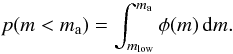 (1)In this work,
the integrals over the IMF will always be read as equal to or larger than the lower
limit and lower than the upper limit. In this work we employ the Kroupa IMF (Kroupa 2001, 2002) as used in Weidner & Kroupa
(2006), with
mup = 120 M⊙,
mlow = 0.01 M⊙, and a
correction of k′ = 1/3 for stars with
mass lower than 0.08 M⊙2.
(1)In this work,
the integrals over the IMF will always be read as equal to or larger than the lower
limit and lower than the upper limit. In this work we employ the Kroupa IMF (Kroupa 2001, 2002) as used in Weidner & Kroupa
(2006), with
mup = 120 M⊙,
mlow = 0.01 M⊙, and a
correction of k′ = 1/3 for stars with
mass lower than 0.08 M⊙2. -
2.
Different observational scenarios can be described by adding constraints to the IMF. For instance, we may explicitly include a limit on ma and compute probabilities for stars with masses lower than ma. In this case, we must define an a posteriori PDF related to the IMF that includes such a condition:
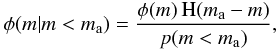 (2)where
H(ma − m) is the Heaviside
function3, which ensures that no star equal to
or larger than ma can be present in the cluster. We note
that
φ(m|m < ma)
is a PDF also. The mean mass of such distribution is
(2)where
H(ma − m) is the Heaviside
function3, which ensures that no star equal to
or larger than ma can be present in the cluster. We note
that
φ(m|m < ma)
is a PDF also. The mean mass of such distribution is 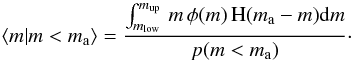 (3)
(3) -
3.
The PDF describing ensembles with a total number of stars
(formally, a sampling distribution conditioned to have
stars) can be calculated as successive convolutions of the corresponding PDF for one
star. For instance, the PDF for the total mass,
 ,
is the result of convolving the IMF
times in a recursive convolution (see Cerviño &
Luridiana 2006; Selman & Melnick
2008):
,
is the result of convolving the IMF
times in a recursive convolution (see Cerviño &
Luridiana 2006; Selman & Melnick
2008): 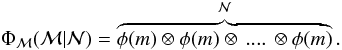 (4)The same procedure
applies to any other PDF. The mean value of the resulting distribution is
(4)The same procedure
applies to any other PDF. The mean value of the resulting distribution is
 (5)Mean values of
constrained distributions when sampled with
stars are obtained in a similar way.
(5)Mean values of
constrained distributions when sampled with
stars are obtained in a similar way.
3. The trade-off between knowledge and probability
Once we have laid down the basic framework, we apply it to our science case: the estimation of the total mass ℳ of a cluster from a partial knowledge of its stellar content. To do that we progressively replace known information by unknowns to describe real situations; however, the following items here are not directly related to the scenarios quoted in the Introduction (we will come back to such scenarios in Sect. 4).
3.1. Case study 1: everything is known
We begin with an ideal observational point of view, where we suppose that we know the
masses  of every
one of the
stars in a cluster. Thus, the total mass, ℳ, is also known. In this hypothetical case, it
is not required to use the IMF. However, this exercise allows us to illustrate the
trade-off between the use of known data from a particular cluster (i.e., a particular IMF
realization) and the use of probability distributions.
of every
one of the
stars in a cluster. Thus, the total mass, ℳ, is also known. In this hypothetical case, it
is not required to use the IMF. However, this exercise allows us to illustrate the
trade-off between the use of known data from a particular cluster (i.e., a particular IMF
realization) and the use of probability distributions.
We sort the stars in ascending order according to their mass. We use a subindex in
brackets to denote that such operation has been performed, so
mi is the ith random
sampled element and m [i] is the
i-th element after sorting the data. We also assume that the most
massive star has a mass ![Mathematical equation: \hbox{$m_{[{\cal N}]}^{\mathrm{obs}} = m_\mathrm{max}^{\mathrm{obs}}$}](/articles/aa/full_html/2013/05/aa20937-12/aa20937-12-eq38.png) with a
value lower than mup.
with a
value lower than mup.
In addition, we assume that we have Na stars equal or more
massive than an arbitrary value ma, so that
![Mathematical equation: \hbox{$m_{[{\cal N}-N_\mathrm{a} ]} < m_\mathrm{a}$}](/articles/aa/full_html/2013/05/aa20937-12/aa20937-12-eq40.png) ,
and
,
and ![Mathematical equation: \hbox{$m_{[{\cal N}-N_\mathrm{a} +1]}\ge m_\mathrm{a}$}](/articles/aa/full_html/2013/05/aa20937-12/aa20937-12-eq41.png) .
We express the total number of stars and total mass as a function of the
Na set. It can be described as
.
We express the total number of stars and total mass as a function of the
Na set. It can be described as
![Mathematical equation: \begin{equation} N_\mathrm{a} = \sum_{i={\cal N}-N_\mathrm{a}+1}^{\cal N} \delta_{i,i}, ~~~~~ M_\mathrm{a} = \sum_{i={\cal N}-N_\mathrm{a}+1}^{\cal N} m_{[i]}^\mathrm{obs} \delta_{i,i}, \end{equation}](/articles/aa/full_html/2013/05/aa20937-12/aa20937-12-eq42.png) (6)where
δi,j is the Kronecker delta. The total
mass in the ensemble is
(6)where
δi,j is the Kronecker delta. The total
mass in the ensemble is ![Mathematical equation: \begin{equation} {\cal M} = M_\mathrm{a} + \sum_{i=1}^{{\cal N}-N_\mathrm{a}} m_{[i]}^{\mathrm{obs}} \delta_{i,i}. \label{eq:MtotKnown} \end{equation}](/articles/aa/full_html/2013/05/aa20937-12/aa20937-12-eq44.png) (7)These two equations,
rewritten in terms of frequencies and mean stellar mass in the complete sample, are,
respectively
(7)These two equations,
rewritten in terms of frequencies and mean stellar mass in the complete sample, are,
respectively 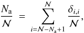 (8)and
![Mathematical equation: \begin{eqnarray} \langle \widetilde{m} \rangle &=& \frac{N_\mathrm{a}}{{\cal N}} \,\, \frac{M_\mathrm{a}}{N_\mathrm{a}} + \frac{{\cal N}-N_\mathrm{a}}{{\cal N}} \sum_{i=1}^{{\cal N}-N_\mathrm{a}} \frac{m_{[i]}^{\mathrm{obs}}}{{\cal N}-N_\mathrm{a}}\cdot \label{eq:frecM} \end{eqnarray}](/articles/aa/full_html/2013/05/aa20937-12/aa20937-12-eq46.png) (9)Multiplying
(9)Multiplying
 by
produces the value of ℳ. However, we note that conceptually
by
produces the value of ℳ. However, we note that conceptually
 (10)since
(the sample mean) does not
coincide with the the mean stellar mass obtained from the IMF, ⟨ m ⟩
(the population mean). That is, is an estimate of
⟨ m ⟩ obtained from a sample of
stars, so, formally,
(10)since
(the sample mean) does not
coincide with the the mean stellar mass obtained from the IMF, ⟨ m ⟩
(the population mean). That is, is an estimate of
⟨ m ⟩ obtained from a sample of
stars, so, formally,  . In the following, we use the
 symbol
to denote an estimate of m. In the computation of this estimate, the
value of
must be taken into consideration, although we will not write it explicitly in order to
simplify the notation.
symbol
to denote an estimate of m. In the computation of this estimate, the
value of
must be taken into consideration, although we will not write it explicitly in order to
simplify the notation.
3.2. Case study 2: the total number of stars and the mass of the most massive Na stars are known
In this case we have less information than in the previous case since we only know
![Mathematical equation: \hbox{$m_{[i]}^{\mathrm{obs}}$}](/articles/aa/full_html/2013/05/aa20937-12/aa20937-12-eq54.png) with
with
 ,
stellar masses, and .
But we had seen that estimates obtained from actual values, such as
can be related to values
obtained from the IMF. So we can replace these estimates with
,
stellar masses, and .
But we had seen that estimates obtained from actual values, such as
can be related to values
obtained from the IMF. So we can replace these estimates with
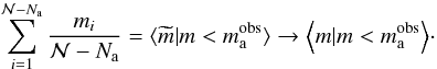 Thus,
although we cannot know the actual ℳ value, we can at least obtain average values given
different sets of constraints:
Thus,
although we cannot know the actual ℳ value, we can at least obtain average values given
different sets of constraints: ![Mathematical equation: \begin{eqnarray} \Big\langle{\cal M} | m_{[i]}^\mathrm{obs} \ge m_\mathrm{a}^\mathrm{obs}\; i&&={\cal{N}} - N_\mathrm{a} +1, ... \cal{N};~{\cal N} \Big\rangle \nonumber\\ \label{eq:frecprobM}&&=M_\mathrm{a} + ({\cal N}-N_\mathrm{a}) \Big\langle m | m < m\mathrm{_{a}^{obs}} \Big\rangle \cdot \end{eqnarray}](/articles/aa/full_html/2013/05/aa20937-12/aa20937-12-eq57.png) (11)This
illustrates the trade-off between observed frequency distributions and probability: when
we use a probability distribution, we cannot have access to the actual values, but we can
have access to the distribution of possible values and the mean value of all these
possible values. In this case we are using the estimates argument in the opposite
direction to a statistical analysis, i.e., we are making the assumption that all the stars
are distributed following the IMF4 and using it to
make inferences about related quantities.
(11)This
illustrates the trade-off between observed frequency distributions and probability: when
we use a probability distribution, we cannot have access to the actual values, but we can
have access to the distribution of possible values and the mean value of all these
possible values. In this case we are using the estimates argument in the opposite
direction to a statistical analysis, i.e., we are making the assumption that all the stars
are distributed following the IMF4 and using it to
make inferences about related quantities.
3.3. Case study 3: only the mass of the Na more massive stars is known
Observations of clusters in many cases only allow characterization of the
Na most luminous stars with masses
![Mathematical equation: \hbox{$m_{[i]}^\mathrm{obs}, \, i=\{{\cal N}-N_\mathrm{a}+1,\dots\,{\cal N}\}$}](/articles/aa/full_html/2013/05/aa20937-12/aa20937-12-eq58.png) . They also lack a proper
census that includes the lowest luminous members (see Bayo
et al. 2011; Kirk & Myers 2011,as
counterexamples). In this case, it is more difficult to obtain estimates, since we can not
define a frequency of Na. Therefore, is the following
reasoning valid?
. They also lack a proper
census that includes the lowest luminous members (see Bayo
et al. 2011; Kirk & Myers 2011,as
counterexamples). In this case, it is more difficult to obtain estimates, since we can not
define a frequency of Na. Therefore, is the following
reasoning valid? 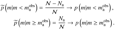
3.3.1. When is the correspondence
= Na/p(m | m
≥ ma) valid?
We divide the IMF in, e.g., k + 1 mass intervals, where the mass
interval containing the lower masses, e.g., the k + 1, comprises the
 of unknown stars with mass lower than ma. Each of the
remaining i mass interval, which belong to
of unknown stars with mass lower than ma. Each of the
remaining i mass interval, which belong to
 contain
ni stars5, so that
contain
ni stars5, so that  . The
probability of having a star in a given mass interval is given by the integration of the
IMF over such a mass interval,
. The
probability of having a star in a given mass interval is given by the integration of the
IMF over such a mass interval,  ). We assume that the cluster
is a random realization of the IMF for
stars, so the probability of having the
stars distributed in the k + 1 intervals with
ni stars in the ith
interval for a given (unknown) number of stars
is given by the multinomial distribution6
). We assume that the cluster
is a random realization of the IMF for
stars, so the probability of having the
stars distributed in the k + 1 intervals with
ni stars in the ith
interval for a given (unknown) number of stars
is given by the multinomial distribution6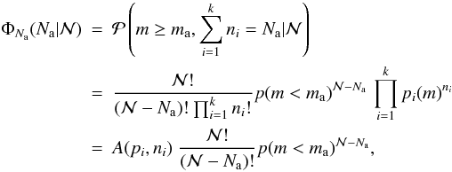 (12)where
we have included in
A(pi,ni)
all the known information. However, we are interested in the complementary distribution
(12)where
we have included in
A(pi,ni)
all the known information. However, we are interested in the complementary distribution
 ,
which must be obtained using the Bayes’ theorem (see, e.g., Paper I). Assuming that the
possible values of ,
,
which must be obtained using the Bayes’ theorem (see, e.g., Paper I). Assuming that the
possible values of ,
 follow a discrete power-law probability distribution with exponent
−β, we obtain
follow a discrete power-law probability distribution with exponent
−β, we obtain 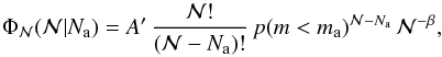 (13)where
A′ is a normalization value that includes all the known
terms and is independent of
A(pi,ni)
since
A(pi,ni)
is canceled out by the normalization constant, Thus, the inference about the total
number of stars only depends on the number of stars Na more
massive than a certain observational value ma, and not on
the particular distribution of such stars in different mass bins.
(13)where
A′ is a normalization value that includes all the known
terms and is independent of
A(pi,ni)
since
A(pi,ni)
is canceled out by the normalization constant, Thus, the inference about the total
number of stars only depends on the number of stars Na more
massive than a certain observational value ma, and not on
the particular distribution of such stars in different mass bins.
This result might seem surprising: the knowledge of the masses of particular stars does not provide additional information on (the number) of unobserved ones7. It can be argued that, for example, an excess or deficit of the observed number of stars in a given mass range constrains the total number of stars from being compatible with sampling effects. However, such arguments are valid for IMF inferences (which IMF shape is more probable, given some observations?), i.e., the problem of obtaining the IMF.
In our case, a given IMF is assumed and the observations are a random realization of it. The particular observed set may be a highly improbable (but still possible) realization of the assumed IMF. Nevertheless, whatever its a priori probability of happening, it has actually happened, and thus a posteriori probabilities must be obtained by taking this fact into consideration. In addition, since stellar masses are random variables (cf. Paper I), the occurrence of having a star (or a set of stars) with a given particular mass has no impact on the individual masses of the remaining stars.
The mode of ,
 is obtained by equating to zero its first derivative with respect to
,
which, for large
values8, yields
is obtained by equating to zero its first derivative with respect to
,
which, for large
values8, yields 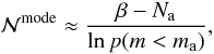 (14)where we used the
Stirling approximation of factorial functions and a first-order Taylor approximation of
logarithm functions valid for β ≠ 0. In the case of a flat distribution
with β = 0, the approximate mode of the distribution is obtained by
solving
(14)where we used the
Stirling approximation of factorial functions and a first-order Taylor approximation of
logarithm functions valid for β ≠ 0. In the case of a flat distribution
with β = 0, the approximate mode of the distribution is obtained by
solving 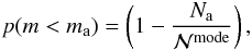 (15)which coincides with
the estimation of the probability
(15)which coincides with
the estimation of the probability  for
known Na and .
This means that
Na/p(m|m ≥ ma)
provides the mode
for
known Na and .
This means that
Na/p(m|m ≥ ma)
provides the mode  of
assuming a flat
distribution. However, we know that the initial cluster mass function (ICMF,
Φℳ(ℳ) ) is not flat (Lada & Lada
2003; Piskunov et al. 2008) and that it
must be somehow related to
(cf. Eq. (4)), although we are not able
to establish its functional form. Whatever equation we use to obtain
,
we are left in the uncomfortable situation of mixing a mean value
(⟨ m|m < ma ⟩ )
with a mode value
to obtain an inference about ℳ. However, we have no means to give a meaning of this
inference: Is it a mean, a mode, on any other parameter?
of
assuming a flat
distribution. However, we know that the initial cluster mass function (ICMF,
Φℳ(ℳ) ) is not flat (Lada & Lada
2003; Piskunov et al. 2008) and that it
must be somehow related to
(cf. Eq. (4)), although we are not able
to establish its functional form. Whatever equation we use to obtain
,
we are left in the uncomfortable situation of mixing a mean value
(⟨ m|m < ma ⟩ )
with a mode value
to obtain an inference about ℳ. However, we have no means to give a meaning of this
inference: Is it a mean, a mode, on any other parameter?
This suggests that it is better to use the resulting probability distribution of
 and obtain the corresponding
 ![Mathematical equation: \hbox{$\Phi_{\cal M}[{\cal M} | N_\mathrm{a}, \Phi_{\cal N}({\cal N})]$}](/articles/aa/full_html/2013/05/aa20937-12/aa20937-12-eq86.png) to make inferences about ℳ. In addition, this way to proceed is in agreement with the
International Organization for Standardization (ISO), which recommends expressing the
uncertainty in the results as a PDF9.
to make inferences about ℳ. In addition, this way to proceed is in agreement with the
International Organization for Standardization (ISO), which recommends expressing the
uncertainty in the results as a PDF9.
4. Use cases
Data form stellar associations by Kirk & Myers (2011).
Having presented the probabilistic framework and the related information trade-off, we can
compare the probabilistic methodology and the distribution by number methodology to obtain ℳ
and .
For comparison purposes, we have used the data from Kirk
& Myers (2011) to illustrate the differences. The data contain the observed
masses for individual stars belonging to 14 young stellar groups in four different regions.
They also contain the stellar mass of field stars in the four analyzed regions. Table 1 shows the identifier of the cluster along with the
values of ℳ, Ma, ,
Na, and the estimation of the mean mass,
 from the census of stars with
m ≥ ma. Kirk
& Myers (2011) state that their mass estimates are valid with a relative
error of 50%; in this work we assume that the tabulated values can be taken at face value
without errors. They also state that their census is complete at a 90% level down to
0.08 M⊙; hence their total mass estimation would be
actually a lower limit of the real value. Whatever the case, we assume again that the ℳ
values obtained from the data can be use at face value without errors. Finally, we assume
that the data is complete at 100% down to
ma = 0.5 M⊙. We use this
ma value to illustrate the ℳ inference in scenarios 2, 3, and
4 in the introduction.
from the census of stars with
m ≥ ma. Kirk
& Myers (2011) state that their mass estimates are valid with a relative
error of 50%; in this work we assume that the tabulated values can be taken at face value
without errors. They also state that their census is complete at a 90% level down to
0.08 M⊙; hence their total mass estimation would be
actually a lower limit of the real value. Whatever the case, we assume again that the ℳ
values obtained from the data can be use at face value without errors. Finally, we assume
that the data is complete at 100% down to
ma = 0.5 M⊙. We use this
ma value to illustrate the ℳ inference in scenarios 2, 3, and
4 in the introduction.
As reference, the IMF used here produces
⟨ m ⟩ = 0.46 M⊙,
⟨ m|m ≥ ma ⟩ = 1.64 M⊙,
and
p(m|m ≥ ma) = 0.19.
We can make a first-order test about the compatibility of the cluster data with the assumed
IMF by computing the probability of having a given Na number of
stars with mass larger than ma in a cluster with
stars. It can be done by dividing the IMF into two bins,
[mlow,ma) and
[ma,mup), and
using the probability in each bin to define a binomial distribution. The logarithm value of
the resulting probabilities normalized to the maximum value of the distribution,
 ,
are shown in Col. 7 of Table 110. In this test we see that our hypothesis about the validity of the
used IMF in all the associations is actually questionable for the stars in Taurus field,
Taurus #4, and IC 348 #1, and would produce some problems in the analysis of Taurus #5, #7,
and #6.
,
are shown in Col. 7 of Table 110. In this test we see that our hypothesis about the validity of the
used IMF in all the associations is actually questionable for the stars in Taurus field,
Taurus #4, and IC 348 #1, and would produce some problems in the analysis of Taurus #5, #7,
and #6.
4.1. Distribution-by-number methodology
The distribution-by-number methodology considers that the IMF can be used with an
arbitrary normalization. Such normalization can be either to
or ℳ, which implies multipling φ(m) by
or ℳ/ ⟨ m ⟩ , respectively. In addition, it is assumed
that
and ℳ are deterministically related by the relation 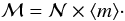 (16)This provides ℳ in
all the cases where
is given and vice versa. We can include additional information like
Ma and Na to make alternative
inferences about ℳ. Following the procedure of this paper, the most information is
included using a formula similar to Eq. (11):
(16)This provides ℳ in
all the cases where
is given and vice versa. We can include additional information like
Ma and Na to make alternative
inferences about ℳ. Following the procedure of this paper, the most information is
included using a formula similar to Eq. (11):  (17)However, we can
choose to use only partial information, such as the contribution of
Ma to the total budget. Then the ratio
ℳ/Ma is constant, and is equal to the
ratio of m × φ(m) integrated in the
whole range, ⟨ m ⟩ , over the same function integrated in the
ma, mup range. As a result, ℳ
is:
(17)However, we can
choose to use only partial information, such as the contribution of
Ma to the total budget. Then the ratio
ℳ/Ma is constant, and is equal to the
ratio of m × φ(m) integrated in the
whole range, ⟨ m ⟩ , over the same function integrated in the
ma, mup range. As a result, ℳ
is: 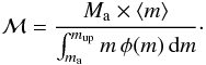 (18)On the other
hand, we could choose to use the contribution of Na to the
total budget. Then the ratio
(18)On the other
hand, we could choose to use the contribution of Na to the
total budget. Then the ratio  is constant and is equal to the ratio of φ(m) integrated
in the whole range (that is, the unity) over the φ(m)
integrated in the ma, mup range.
Since
is constant and is equal to the ratio of φ(m) integrated
in the whole range (that is, the unity) over the φ(m)
integrated in the ma, mup range.
Since  ,
ℳ is
,
ℳ is  (19)We could also
choose to use just Ma and Na
values without the information about
(similar to Eq. (17) with some additional
algebraic manipulation):
(19)We could also
choose to use just Ma and Na
values without the information about
(similar to Eq. (17) with some additional
algebraic manipulation):  (20)Equations (18)–(20) produce an equal value of ℳ as far as
  and
they will produce a result similar to Eqs. (16) and (17) as far as,
additionally,
and
they will produce a result similar to Eqs. (16) and (17) as far as,
additionally,  In
relation to the scenarios presented in the Introduction, scenario 2 (only
is observed) is described by Eq. (16).
Scenario 3 (,
Na, and Ma are known) can be
described by Eqs. (16)–(20), depending the information we choose to
use, with Eq. 17 being the one that uses
the most available information. Finally, scenario 4 can be described by Eqs. (18)–(20), with Eq. (20) being the one
that use the most available information.
In
relation to the scenarios presented in the Introduction, scenario 2 (only
is observed) is described by Eq. (16).
Scenario 3 (,
Na, and Ma are known) can be
described by Eqs. (16)–(20), depending the information we choose to
use, with Eq. 17 being the one that uses
the most available information. Finally, scenario 4 can be described by Eqs. (18)–(20), with Eq. (20) being the one
that use the most available information.
The resulting ℳ estimations from Kirk & Myers
(2011) data employing this methodology are shown in Table 2, which uses different information from the cluster. The inferred ℳ
varies depending on the formulae (and hence the amount of not redundant information) used
for the inference. The best result is obtained by Eq. (17), but unfortunately it does not have a practical application
(
is unknown most of the times).
With respect to the equations that can be used in scenario 4 (the common observational
case), Eq. (20) produce a value between
the results of Eqs. (18) and (19). Also, since
 underestimates
⟨m|m ≥ ma⟩ for the
clusters in the given sample, Eq. (18)
produces lower values than Eq. (19) (see
Taurus #8 as the opposite example). The range of inferred ℳ values covered by Eqs. (18)–(20) only include the observed ℳ value in four cases (Taurus #8, Cha #1 and #2,
and the field stars in IC 348), suggesting a 20% rate of success (33% if we exclude the
five clusters with possible strong deviations from the assumed IMF). In addition, we do
not known which equation produces the more reasonable value (although Eq. (20) is preferred) nor do we have a possible
evaluation accuracy associated to each case.
underestimates
⟨m|m ≥ ma⟩ for the
clusters in the given sample, Eq. (18)
produces lower values than Eq. (19) (see
Taurus #8 as the opposite example). The range of inferred ℳ values covered by Eqs. (18)–(20) only include the observed ℳ value in four cases (Taurus #8, Cha #1 and #2,
and the field stars in IC 348), suggesting a 20% rate of success (33% if we exclude the
five clusters with possible strong deviations from the assumed IMF). In addition, we do
not known which equation produces the more reasonable value (although Eq. (20) is preferred) nor do we have a possible
evaluation accuracy associated to each case.
Inference of ℳ employing the distribution-by-number methodology in the stellar associations by Kirk & Myers (2011), according different scenarios.
4.1.1. The probabilistic methodology
In the probabilistic case, PDFs are only used to describe unknown data, and observed
data is used to define constraints over such unknown data, so that both types of data
have different roles. In addition, the solution cannot be summarized in a single value,
but as a distribution function. Although some summaries of such distribution (as the
mean value) can be obtained analytically, such values do not necessarily have enough
information, and the best method is to obtain the full distribution of possible
solutions and work with it. We propose here the methodology to obtain the probability
distribution of ℳ when we know the individual masses of the most massive
Na stars, and we know that all stars equal to or more
massive than  are
included in the Na set. The problem cannot be solved
analytically since recursive convolutions involving power laws (such as the IMF) have no
analytical solution. So we can only propose the following step-by-step procedure:
are
included in the Na set. The problem cannot be solved
analytically since recursive convolutions involving power laws (such as the IMF) have no
analytical solution. So we can only propose the following step-by-step procedure:
-
1.
Obtain the distribution of
,
 ,
which can be inferred from the datausing Eq. (13). We stress again that an assumptionabout
is required. We note that the result would be quite dependenton the lower limit
assumed in the
distribution.
,
which can be inferred from the datausing Eq. (13). We stress again that an assumptionabout
is required. We note that the result would be quite dependenton the lower limit
assumed in the
distribution. -
2.
Compute the distribution of ΦMnot−obs(Mnot−obs|Ni) for the possible values of
 values obtained from the previous distribution. The distribution provides the
distribution of possible values of the total mass from the unknown stars,
Mnot−obs, that is, ℳ is actually constrained to the
non-observed stellar masses
values obtained from the previous distribution. The distribution provides the
distribution of possible values of the total mass from the unknown stars,
Mnot−obs, that is, ℳ is actually constrained to the
non-observed stellar masses  , so we
must use a constrained IMF to describe what we do not know,
φ(m|m < ma).
Such
ΦMnot−obs(Mnot−obs|Ni)
distributions can be computed either by Monte Carlo simulations or by a numerical
self-convolution.
, so we
must use a constrained IMF to describe what we do not know,
φ(m|m < ma).
Such
ΦMnot−obs(Mnot−obs|Ni)
distributions can be computed either by Monte Carlo simulations or by a numerical
self-convolution. -
3.
Compute the distribution of Φℳ(ℳ|Ma,Na). This is done by weighting the previous ΦMnot−obs(Mnot−obs|Ni) distributions by the probabilities of each Ni value provided by
and including the contribution to the total mass of the observed stars.
to obtain different Ni values, and by
sampling the constrained IMF with this number of stars. The previous procedure covers
scenarios 2 and 3 by applying only step 2: obtain
 or
Φℳ(ℳnot−obs|Ni)
for a known .
or
Φℳ(ℳnot−obs|Ni)
for a known .
We applied this methodology to the set of clusters of Kirk & Myers (2011) under different scenarios by means of Monte Carlo
simulations. The distribution of solutions for each cluster in each scenario was sampled
by 107 Monte Carlo simulations, and the resulting distribution was binned in
intervals with Δℳ = 0.5 M⊙. We note that in scenario 4
the simulations sample both the IMF and the assumed
distributions (power laws with β = 0 and β = 2).
Therefore, the simulations span a larger ℳ range and an additional uncertainty is
expected for the confidence interval estimations.
Inference of ℳ employing probabilistic methodology for the stellar associations
by Kirk & Myers (2011) in
scenario 2, using the observed value of .
Table 3 shows the resulting mean, mode, and 68.3% (equivalent to 1σ in a Gaussian distribution) and 95.4% (equivalent to 2σ in a Gaussian distribution) confidence intervals around the mode for scenario 2. As expected, the mean value of the distribution coincides with the result of Eq. (16) shown in Table 2. All observed ℳ are in the 94.5% confidence interval around the mode, although only 27% are in the 68.3% confidence interval, being the observed ℳ larger than the range quoted in such interval.
Inference of ℳ employing probabilistic methodology for the stellar associations
by Kirk & Myers (2011) in
scenario 3, using the observed value of ,
Na, Ma and
ma = 0.5 M⊙.
Table 4 shows the results of the ℳ distribution for scenario 3, which includes a larger amount of information. The mean and mode of the distribution coincides (hence the distribution is symmetric), and the mean value is also coincident to the result of Eq. (17), as expected. However, in this case we can evaluate how good this estimation actually is (and hence the distribution by number estimation). Taking favorable round-around cases, 17% of the clusters (i.e., field stars in ChaI, IC 348 #1, and field stars in IC 348) are outside the 2σ range, 83% are in the 2σ range, and 67% are in the 1σ range (i.e., 12 clusters). Given the low number of clusters for this study, we find this result partially consistent with a standard methodology. However, in theory, we would expect only one cluster outside the 2σ range, although we can invoke the use of a low number of clusters for this study. An additional outcome of this study is that, although Eq. (17) produces results similar to the observations, it does not necessarily provide a fully compatible (e.g., at 1σ level) result. Again, this enforces the idea of using the whole PDF of possible solutions instead a summary (like the confidence interval range) of it.
Inference of ℳ employing probabilistic methodology for the stellar associations
by Kirk & Myers (2011), using the
value of Na, Ma and
ma = 0.5 M⊙ and
assuming a flat
distribution.
Inference of ℳ employing probabilistic methodology for the stellar associations
by Kirk & Myers (2011), using the
value of Na, Ma and
ma = 0.5 M⊙ and
assuming a power-law
distribution with β = 2.
Tables 5 and 6 show the results of applying this methodology using flat and power law
distributions (β = 0 and β = 2, respectively) in the
range from  to
to  stars. The first result is that mean and mode values of the distribution are not equal
in general, and the distribution is not symmetric, but j-shaped. The
mode in the case of a flat
distribution is similar to the result obtained by Eq. (20). In this case, the observed ℳ of seven clusters are outside the
2σ confidence interval (actually, the clusters with lower
stars. The first result is that mean and mode values of the distribution are not equal
in general, and the distribution is not symmetric, but j-shaped. The
mode in the case of a flat
distribution is similar to the result obtained by Eq. (20). In this case, the observed ℳ of seven clusters are outside the
2σ confidence interval (actually, the clusters with lower
 value quoted before and ChaI#3). If we neglect the six clusters with the larger
deviations from the IMF, we obtain a result showing that 9% of the cluster are outside
the 2σ interval, 91% of the cluster are in the 2σ
interval, and 55% of the clusters are in the 1σ interval. This is a
reasonable result of any statistical test.
value quoted before and ChaI#3). If we neglect the six clusters with the larger
deviations from the IMF, we obtain a result showing that 9% of the cluster are outside
the 2σ interval, 91% of the cluster are in the 2σ
interval, and 55% of the clusters are in the 1σ interval. This is a
reasonable result of any statistical test.
Finally, the results of Eqs. (18) and
(20) are within the
2σ range in the case of a flat
distribution, but the results of Eq. (19) (estimation from the extrapolations of the observed
Na) produce larger values than the upper limit of
2σ.
5. Discussion
We have shown in this work that the determination of cluster masses is not so trivial as supposed in the literature. The distribution-by-number methodology uses known data to determine unknown data, whereas the probabilistic methodology uses known data to constrain unknown data. The problem is also related to the trade-off between unknown data and probability. When we use a PDF, like the IMF, to make inferences about unknown data, we implicitly renounce obtaining actual values of the inferred quantity. The price is to renounce precision in favor of accuracy. In contrast, the distribution-by-number methodology favors precision and renounces accuracy. The difference is in the algebra (and the logic reasoning) used in each of the methodologies to manipulate formulae. The distribution-by-number methodology uses standard algebra, where symbols are just mathematical expressions without added meaning. The probabilistic methodology follows the algebra of probability, which implies a clear identification of the known and the (random) variables we aim to describe by a probability distribution.
As an example, the equation  provides
an estimation of the number of stars with mass equal or larger than
provides
an estimation of the number of stars with mass equal or larger than
 in
a cluster with
stars. But such an estimation is not necessarily a mean value nor a mode value (cf. Paper I
for the case that Na = 1). In that case, we know
;
hence, we are working with a
in
a cluster with
stars. But such an estimation is not necessarily a mean value nor a mode value (cf. Paper I
for the case that Na = 1). In that case, we know
;
hence, we are working with a  distribution. The inversion of the equation, that is,
  provides
the modal value
of the distribution
provides
the modal value
of the distribution  when a flat distribution of
values is assumed, (i.e.,
when a flat distribution of
values is assumed, (i.e.,  .
The distribution
appears naturally when the Bayes’ theorem is used. This is a natural result when we realize
that, since
is unknown, we need its probability distribution to make inferences about it, and that the
“innocent” algebraic manipulation we have done has a completely different meaning than the
one we would expect.
.
The distribution
appears naturally when the Bayes’ theorem is used. This is a natural result when we realize
that, since
is unknown, we need its probability distribution to make inferences about it, and that the
“innocent” algebraic manipulation we have done has a completely different meaning than the
one we would expect.
5.1. To
or not to ?
We are now in the uncomfortable situation of having to assume a
distribution in the inference of
and ℳ. However, the relevance of the
in the inference of ℳ is also dependent on the value of ma and
Na. In a back-of-the-envelope argument, the effect of a
power-law
distribution is to decrease Na by β stars
(cf. Eq. (14) used for
estimation). Hence, the larger Na, the lower the dependence of
the ℳ estimation on .
Of course, the way to increase Na is to be complete down to
the lowest ma possible.
In the cases where the ℳ inference strongly depends on our choice of
,
we must be guided by our knowledge of the physical system environment and the scientific
goal of the analysis. A flat
assumes that there is no previous knowledge about the system environment, so it looks like
good option in the case of isolated systems and when we are only interested in the system
properties.
However, the situation varies if we are interested in a cluster that we know is in a
supercluster environment or is the result of molecular cloud fragmentation. In these
cases, depending on our knowledge and hypothesis about star formation (SF), we can
consider that such fragmentation is the result of a high-order structure; hence, the
particular cluster is not an isolated entity. This would imply that some values of
or ℳ are more probable than others, and this information must be taken into account in the
inference of
and ℳ of the particular cluster.
We must stress here that the proposed method only applies to
distributions, and not to Φℳ(ℳ) ones. The case of
is easily implemented as far as it is related to sampling theory and the number of the
elements in the sample is the relevant quantity. The inclusion of Φℳ(ℳ) is not
so trivial, since it depends implicitly on a
distribution. However, such distribution can not be obtained analytically (the convolution
problem is not analytic in general cases). In addition, since
is a discrete distribution, we have a large, but finite (and hence computable), number of
cases. This is not true for Φℳ(ℳ) because it is a continuous function and the
possible solutions that a combination of
stars produces a particular ℳ is infinite. At this moment, the only solution is to use
Φℳ(ℳ) as a proxy for ,
which would be valid for situations where we know a priori that the minimum possible
number of stars is large (i.e., Na is large, or we have
additional information about a minimum number of stars in the cluster).
Finally, the situation also changes if we are interested in obtaining
or Φℳ(ℳ) from a set of clusters. Following Tarantola (2006), the most viable way is to make an iterative process. First,
assume a  distribution and compute resulting distributions of
 and ℳi for each cluster. After that, combine such
distributions to obtain from the sample the global distributions
and ℳi for each cluster. After that, combine such
distributions to obtain from the sample the global distributions
 and Φℳ,1(ℳ). If
  ,
then
is not a self-consistent hypothesis. However, we must be aware that this does not prove
that
and Φℳ,1(ℳ) are self-consistent hypotheses! The only way to
achieve a self-consistent hypothesis is iterate the process until
,
then
is not a self-consistent hypothesis. However, we must be aware that this does not prove
that
and Φℳ,1(ℳ) are self-consistent hypotheses! The only way to
achieve a self-consistent hypothesis is iterate the process until
 being the j − 1 distribution is the one used as input and the
j distribution is the resulting one, along with testing if the
resulting Φℳ,j(ℳ) distributions also obey such a condition (a
cross validation). However, we stress again that such a cross-validation process is a
requirement that depends on the Na value and that for large
enough Na values, the resulting
Φℳ(ℳ|Ma,Na)
solution for the ℳ distribution of a cluster is almost
independent.
being the j − 1 distribution is the one used as input and the
j distribution is the resulting one, along with testing if the
resulting Φℳ,j(ℳ) distributions also obey such a condition (a
cross validation). However, we stress again that such a cross-validation process is a
requirement that depends on the Na value and that for large
enough Na values, the resulting
Φℳ(ℳ|Ma,Na)
solution for the ℳ distribution of a cluster is almost
independent.
6. Conclusions
Throughout this work, we have explicitly developed the use of the IMF to obtain different physical parameters of stellar systems from limited information. We made extensive use of the IMF as a PDF, which allowed us to make proper use of probability theory and, in particular, the properties of sampling distributions (where the total number of stars in the system is included) and conditional probabilities.
We studied the methodology to obtain the distribution of possible
and ℳ values from the knowledge of the set of the most massive stars in the system. The
result is dependent on the values of ma and
Na, and on the hypothesis about the overall distribution of
the number of stars in clusters ,
including the limits of such distribution (especially the lower one).
This definition implies that stellar masses are identically and independent distributed, we refer Paper I for more details.
Such a correction was not used in Paper I. However, it is the parametrization used in the set of clusters by Kirk & Myers (2011) we use in this work for comparing methodologies.
We use here the Heaviside function as a distribution to define the domain of φ(m) including constraints. In this situation the value of H(0) is not defined, but it is assigned a posteriori to be consistent with the convention used in the integral limits. In the case of Eq. (2), H(0) = 0.
Hence, it includes the Na subset with known stellar masses.
In this case, we are distributing the known Na stars in
k intervals and not using the particular m values of
known stars. Such intervals can be arbitrary and must only obey the condition
. So the index
i here refers to the interval, not to a particular stellar mass.
Since
is a discrete quantity, their PDF directly provides the probability. In addition, the
distribution can be also expressed as a binomial distribution with
A(pi,ni) Na ! = p(m ≥ ma)Na = (1 − p(m < ma))Na.
However, we note that such information is still relevant for the computation of ℳ: the individual masses of stars more massive than ma provide the amount of mass in the mass range, Ma.
In practical terms it implies large Na values. Actually,
is a discrete distribution, hence not derivable, but the formulae provide a reasonable
value as far as the Stirling approximation of factorial functions are valid, i.e.,
,
Na, and  larger than 15.
Guide to the Expression of Uncertainty in Measurement (International Organization for Standardization, Switzerland, 1995) http://www.bipm.org/en/publications/guides/gum.html
We note that a comparison of  and
p(m|m ≥ ma)
does not produce a valid test about IMF compatibility, since the importance of the
possible deviations depends on how many stars are in the sample (size of sample effects).
Interestingly, IC 348 #1, which deviates from the IMF in this test, is the system used as
an example by Kirk & Myers (2011) to argue
that their systems follows a Kroupa IMF (their Fig. 6). Although the shape of the IMF
realization in IC 348#1 would look like a Korupa IMF, the deviations (fluctuations)
observed are actually too large compared with the expected ones taking into account the
number of stars in the system.
and
p(m|m ≥ ma)
does not produce a valid test about IMF compatibility, since the importance of the
possible deviations depends on how many stars are in the sample (size of sample effects).
Interestingly, IC 348 #1, which deviates from the IMF in this test, is the system used as
an example by Kirk & Myers (2011) to argue
that their systems follows a Kroupa IMF (their Fig. 6). Although the shape of the IMF
realization in IC 348#1 would look like a Korupa IMF, the deviations (fluctuations)
observed are actually too large compared with the expected ones taking into account the
number of stars in the system.
Acknowledgments
We acknowledge Kevin Covey for discussions of the similarities and differences of
and Φℳ(ℳ) and their implications in the modeling of clusters and galaxies, which
have been very useful for this paper and related works. We acknowledge the suggestions of
the referee, Peter Anders, which greatly improved the clarity of the paper. This work has
been supported by the MICINN (Spain) through the grants AYA2007-64712, AYA2010-15081,
AYA2010-15196, AYA2011-22614, AYA2011-29754-C03-01, AYA2008-06423-C03-01/ESP, AYA2010-17631,
programs UNAM-DGAPA-PAPIIT IA101812 and CONACYT 152160, Mexico, and co-funded under the
Marie Curie Actions of the European Commission (FP7-COFUND)
References
- Bayo, A., Barrado, D., Stauffer, J., et al. 2011, A&A, 536, A63 [NASA ADS] [CrossRef] [EDP Sciences] [Google Scholar]
- Briceño, C., Luhman, K. L., Hartmann, L., Stauffer, J. R., & Kirkpatrick, J. D. 2002, ApJ, 580, 317 [NASA ADS] [CrossRef] [Google Scholar]
- Bouvier, J., Stauffer, J. R., Martin, E. L., et al. 1998, A&A, 336, 490 [NASA ADS] [Google Scholar]
- Cerviño, M., & Luridiana, V. 2006, A&A, 451, 475 [NASA ADS] [CrossRef] [EDP Sciences] [Google Scholar]
- Cerviño, M., Román-Zuñiga, C., Luridiana, V., et al. 2013, A&A, 553, A31 [NASA ADS] [CrossRef] [EDP Sciences] [Google Scholar]
- Kirk, H., & Myers, P. C. 2011, ApJ, 727, 64 [NASA ADS] [CrossRef] [Google Scholar]
- Kroupa, P. 2001, MNRAS, 322, 231 [NASA ADS] [CrossRef] [Google Scholar]
- Kroupa, P. 2002, Science, 295, 82 [NASA ADS] [CrossRef] [PubMed] [Google Scholar]
- Lada, C. J., & Lada, E. A. 2003, ARA&A, 41, 57 [NASA ADS] [CrossRef] [Google Scholar]
- Luhman, K. L., Stauffer, J. R., Muench, A. A., et al. 2003, ApJ, 593, 1093 [NASA ADS] [CrossRef] [Google Scholar]
- Oliveira, J. M., Jeffries, R. D., & van Loon, J. T. 2009, MNRAS, 392, 1034 [NASA ADS] [CrossRef] [Google Scholar]
- Piskunov, A. E., Kharchenko, N. V., Schilbach, E., et al. 2008, A&A, 487, 557 [NASA ADS] [CrossRef] [EDP Sciences] [Google Scholar]
- Scalo, J. M. 1986, Fun. Cosm. Phys., 11, 1 [Google Scholar]
- Selman, F. J., & Melnick, J. 2008, ApJ, 689, 816 [NASA ADS] [CrossRef] [Google Scholar]
- Tarantola, A. 2006, Nat. Phys., 2, 492 [CrossRef] [Google Scholar]
- Weidner, C., & Kroupa, P. 2006, MNRAS, 365, 1333 [NASA ADS] [CrossRef] [Google Scholar]
All Tables
Inference of ℳ employing the distribution-by-number methodology in the stellar associations by Kirk & Myers (2011), according different scenarios.
Inference of ℳ employing probabilistic methodology for the stellar associations
by Kirk & Myers (2011) in
scenario 2, using the observed value of .
Inference of ℳ employing probabilistic methodology for the stellar associations
by Kirk & Myers (2011) in
scenario 3, using the observed value of ,
Na, Ma and
ma = 0.5 M⊙.
Inference of ℳ employing probabilistic methodology for the stellar associations
by Kirk & Myers (2011), using the
value of Na, Ma and
ma = 0.5 M⊙ and
assuming a flat
distribution.
Inference of ℳ employing probabilistic methodology for the stellar associations
by Kirk & Myers (2011), using the
value of Na, Ma and
ma = 0.5 M⊙ and
assuming a power-law
distribution with β = 2.
Current usage metrics show cumulative count of Article Views (full-text article views including HTML views, PDF and ePub downloads, according to the available data) and Abstracts Views on Vision4Press platform.
Data correspond to usage on the plateform after 2015. The current usage metrics is available 48-96 hours after online publication and is updated daily on week days.
Initial download of the metrics may take a while.