© ESO, 2013

1. Introduction

Observations of the absorbed γ-ray component from high energy blazars have in recent times been used to provide constraints on the physical parameters of the intergalactic medium (IGM) such as the density of optical/infrared radiation backgrounds (Franceschini et al. 2008; Orr et al. 2011). Furthermore, the subsequent electromagnetic cascade produced in the IGM (Aharonian et al. 1994) provides the opportunity to probe the intergalactic magnetic field (IGMF) strength (Plaga 1995; Neronov & Semikoz 2007; Ichiki et al. 2008; Murase et al. 2008; Takahashi et al. 2008). Recent negative results on the search of the secondary γ-ray emission from the γ-ray induced electromagnetic cascades in the GeV energy band have been used to derive lower bounds on the IGMF strength and correlation length (Neronov & Vovk 2010; Tavecchio et al. 2011; Dermer et al. 2011; Taylor et al. 2011; Vovk et al. 2012). Furthermore, such fields must necessarily permeate a significant fraction (>60%) of the column depth to the blazar in order to exert a sufficient effect on the electromagnetic cascade development (Dolag et al. 2011). Thus, combining the obtained lower bounds with the known upper bounds from radio data and theoretical considerations, one finds that the allowed range of IGMF parameters spans several decades in both strength (10^-17 < B < 10^-9 G) and correlation length (10¹³ < λ_B < 10²⁸ cm) parameter space.

The allowed region of (B,λ_B) parameter space is consistent with various intergalactic magnetic field generation scenarios, from phase transitions in the Early Universe (Hogan 1983; Quashnock et al. 1989; Vachaspati 1991; Sigl et al. 1997) to supernova and AGN generated outflows from the galaxies during the recent Cosmological epoch (Bertone et al. 2006). In general, relic cosmological magnetic fields from phase transitions in the Early Universe are expected to have short correlation lengths which depend on the magnetic field strength ${\mathit{\lambda }}_{\mathit{B,}\mathrm{PT}}\mathrm{~}\mathrm{50}\left[\frac{\mathit{B}}{{\mathrm{10}}^{-9}\mathrm{G}}\right]\mathrm{kpc}$(1)which corresponds to the largest processed eddy scale-length at the end of the radiation dominated epoch (Banerjee & Jedamzik 2004). An exception to this rule are magnetic fields produced during the epoch of inflation. In this case the initial correlation length of magnetic field could be arbitrarily large, so that the correlation length of the remaining magnetic field at zero cosmological redshift might also be arbitrarily large. However, the largest processed scale-length still limits the correlation length of the relic inflationary magnetic field to be ${\mathit{\lambda }}_{\mathit{B,}\mathrm{inflation}}\gtrsim \mathrm{50}\left[\frac{\mathit{B}}{{\mathrm{10}}^{-9}\mathrm{G}}\right]\mathrm{kpc}$.

In comparison, magnetic fields generated by galaxy outflows at the late stages of the Universe’s evolution are expected to have correlation lengths of the order of typical galaxy sizes $\mathrm{10}\mathrm{kpc}\lesssim {\mathit{\lambda }}_{\mathit{B,}\mathrm{gal}}\lesssim \mathrm{100}\mathrm{kpc}\mathit{.}$(2)Different possible scenarios for the generation of intergalactic magnetic field can potentially be distinguished through the measurement of λ_B. In what follows we show that gamma-ray measurements of emission from electromagnetic cascades in the intergalactic medium can provide a measurement of magnetic field correlation length if it lies within the range 10  kpc ≲ λ_B ≲ 1 Mpc and provide upper or lower bounds on λ_B outside this range for all measurable values of magnetic field strength B. We note that the effects of plasma physics on cascade development within the voids, the importance of which remains unresolved (Broderick et al. 2012; Schlickeiser et al. 2012; Miniati & Elyiv 2012), are neglected in this work.

2. IGMF coherence length from the source angular profile

Pencil beam model – In order to derive simplified analytic expressions for cascade quantities, we start with the two-generation model depicted in Fig. 1. Considering a narrow beam of γ-rays emitted by a source S in a direction SJ misaligned with the line of sight SO (Fig. 1). For simplicity, we suppose that the primary very-high-energy (VHE) γ-ray beam consists of photons with the same energy E_γ0 emitted by the source S at constant rate of N₀γ-rays per unit time.

Interaction of the VHE γ-rays with extragalactic background light (EBL) leads to their absorption. As a result, the number of photons along the primary γ-ray beam decreases with distance as N(r) = N₀exp⁽ − r/D_γ0⁾, where D_γ0 is the mean free path of γ-rays through the EBL. Each primary photon produces two electrons, so that the rate of injection of e⁺e⁻ pairs along the γ-ray beam is $\frac{\mathrm{d}{\mathit{N}}_{\mathrm{e}}}{\mathrm{d}\mathit{r}}\mathrm{=}\frac{\mathrm{2}{\mathit{N}}_{\mathrm{0}}}{{\mathit{D}}_{{\mathit{\gamma }}_{\mathrm{0}}}}\exp \left(\mathrm{-}\frac{\mathit{r}}{{\mathit{D}}_{{\mathit{\gamma }}_{\mathrm{0}}}}\right)\mathrm{·}$(3)The subsequent cooling of these e⁺e⁻ pairs due to the inverse Compton (IC) scattering of the cosmic microwave background (CMB) photons leads to emission of the secondary γ-ray photons with energies ${\mathit{E}}_{\mathit{\gamma }}\mathrm{\simeq }\mathrm{1}{}^{\mathrm{(}}\mathit{E}_{{\mathit{\gamma }}_{\mathrm{0}}}\mathit{/}\mathrm{1}\mathrm{TeV}{}^{\mathrm{)}}\mathrm{GeV}$. We suppose that the corresponding cooling distance ${\mathit{D}}_{\mathrm{e}}\mathrm{\simeq }\mathrm{0.2}{\left(\frac{{\mathit{E}}_{\mathit{\gamma }}}{\mathrm{1}\mathrm{GeV}}\right)}^{\mathrm{-}\mathrm{1}\mathit{/}\mathrm{2}}\mathrm{Mpc}$(4)is much smaller than distance to the source D. This means that the energy absorbed from the initial beam is emitted in situ, immediately after absorption.

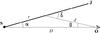Fig. 1 Geometry of cascade emission from a blazar jet SJ misaligned with the line of sight SO.

The conservation of energy demands that the total power of IC emission from the e⁺e⁻ pairs is equal to the power removed from the primary γ-ray beam: 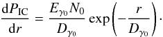$\frac{\mathrm{d}{\mathit{P}}_{\mathrm{IC}}}{\mathrm{d}\mathit{r}}\mathrm{=}\frac{{\mathit{E}}_{{\mathit{\gamma }}_{\mathrm{0}}}{\mathit{N}}_{\mathrm{0}}}{{\mathit{D}}_{{\mathit{\gamma }}_{\mathrm{0}}}}\exp \left(\mathrm{-}\frac{\mathit{r}}{{\mathit{D}}_{{\mathit{\gamma }}_{\mathrm{0}}}}\right)\mathrm{·}$(5)In the presence of IGMF, electrons and positrons are deflected from their original directions. The deflection angle of these pairs depends on the correlation length of magnetic field, λ_B. Two different deflection regimes can be identified:

“One cell” regime – (D_e ≪ λ_B). In this case, the e⁺e⁻ pairs move in nearly homogeneous magnetic field. The deflection angle changes as $\mathit{\delta }\mathrm{\left(}\mathit{x}\mathrm{\right)}\mathrm{=}\frac{\mathit{x}}{{\mathit{R}}_{\mathrm{L}}}$(6)where x is the coordinate along the electron trajectory counted from the pair production point and R_L = E_e/eB is the Larmor radius. As the characteristic value of x is D_e, the previous equation can be rewritten as: 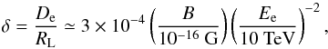$\mathit{\delta }\mathrm{=}\frac{{\mathit{D}}_{\mathrm{e}}}{{\mathit{R}}_{\mathrm{L}}}\mathrm{\simeq }\mathrm{3}\mathrm{\times }{\mathrm{10}}^{-4}\left(\frac{\mathit{B}}{{\mathrm{10}}^{-16}\mathrm{G}}\right){\left(\frac{{\mathit{E}}_{\mathrm{e}}}{\mathrm{10}\mathrm{TeV}}\right)}^{-2}\mathit{,}$(7)

“Many cells” regime – (D_e ≫ λ_B). In this case particles move through many regions with different orientations of magnetic field. Under such conditions electrons and positrons experience random walks in angle, so that the average deflection angle is given by: 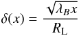$\mathit{\delta }\mathrm{\left(}\mathit{x}\mathrm{\right)}\mathrm{=}\frac{\sqrt{{\mathit{\lambda }}_{\mathit{B}}\mathit{x}}}{{\mathit{R}}_{\mathrm{L}}}$(8)or, substituting x = D_e: 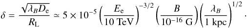$\mathit{\delta }\mathrm{=}\frac{\sqrt{{\mathit{\lambda }}_{\mathit{B}}{\mathit{D}}_{\mathrm{e}}}}{{\mathit{R}}_{\mathrm{L}}}\mathrm{\simeq }\mathrm{5}\mathrm{\times }{\mathrm{10}}^{-5}{\left(\frac{{\mathit{E}}_{\mathrm{e}}}{\mathrm{10}\mathrm{TeV}}\right)}^{\mathrm{-}\mathrm{3}\mathit{/}\mathrm{2}}\left(\frac{\mathit{B}}{{\mathrm{10}}^{-16}\mathrm{G}}\right){\left(\frac{{\mathit{\lambda }}_{\mathit{B}}}{\mathrm{1}\mathrm{kpc}}\right)}^{\mathrm{1}\mathit{/}\mathrm{2}}\mathrm{·}$(9)The deflections of electrons¹ by the IGMF determine the angular pattern of the IC emission. The angular distribution of electrons at each point along the beam can be written in the following way: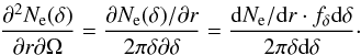$\frac{{\mathit{\partial }}^{\mathrm{2}}{\mathit{N}}_{\mathrm{e}}\mathrm{\left(}\mathit{\delta }\mathrm{\right)}}{\mathit{\partial r\partial }\mathrm{\Omega }}\mathrm{=}\frac{\mathit{\partial }{\mathit{N}}_{\mathrm{e}}\mathrm{\left(}\mathit{\delta }\mathrm{\right)}\mathit{/}\mathit{\partial r}}{\mathrm{2}\mathit{\pi \delta \partial \delta }}\mathrm{=}\frac{\mathrm{d}{\mathit{N}}_{\mathrm{e}}\mathit{/}\mathrm{d}\mathit{r}\mathrm{·}{\mathit{f}}_{\mathit{\delta }}\mathrm{d}\mathit{\delta }}{\mathrm{2}\mathit{\pi \delta }\mathrm{d}\mathit{\delta }}\mathrm{·}$(10)The factor f_δdδ here denotes the fraction of the total number of particles, that were deflected within the range [δ:δ + dδ], and N_e(δ) is the corresponding number of electrons. We assume here, that the probability density function f_x for the electron to emit secondary γ ray is constant over its trajectory and drops to zero at x = D_e. The dependence of this density function on the deflection angle can then be written in the following way: 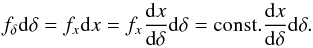${\mathit{f}}_{\mathit{\delta }}\mathrm{d}\mathit{\delta }\mathrm{=}{\mathit{f}}_{\mathit{x}}\mathrm{d}\mathit{x}\mathrm{=}{\mathit{f}}_{\mathit{x}}\frac{\mathrm{d}\mathit{x}}{\mathrm{d}\mathit{\delta }}\mathrm{d}\mathit{\delta }\mathrm{=}\mathrm{const}\mathit{.}\frac{\mathrm{d}\mathit{x}}{\mathrm{d}\mathit{\delta }}\mathrm{d}\mathit{\delta }\mathit{.}$(11)The constant here is defined through the requirement that ${{}^{\mathrm{\int }}}_{\mathrm{0}}^{{\mathit{D}}_{\mathrm{e}}}{\mathit{f}}_{\mathit{x}}\mathrm{d}\mathit{x}\mathrm{=}\mathrm{1}$. We thus can rewrite Eq. (10) in the following way: 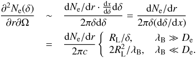$\begin{array}{ccc}\frac{{\mathit{\partial }}^{\mathrm{2}}{\mathit{N}}_{\mathrm{e}}\mathrm{\left(}\mathit{\delta }\mathrm{\right)}}{\mathit{\partial r\partial }\mathrm{\Omega }}& \mathrm{~}& \frac{\mathrm{d}{\mathit{N}}_{\mathrm{e}}\mathit{/}\mathrm{d}\mathit{r}\mathrm{·}\frac{\mathrm{d}\mathit{x}}{\mathrm{d}\mathit{\delta }}\mathrm{d}\mathit{\delta }}{\mathrm{2}\mathit{\pi \delta }\mathrm{d}\mathit{\delta }}\mathrm{=}\frac{\mathrm{d}{\mathit{N}}_{\mathrm{e}}\mathit{/}\mathrm{d}\mathit{r}}{\mathrm{2}\mathit{\pi \delta }\mathrm{(}\mathrm{d}\mathit{\delta }\mathit{/}\mathrm{d}\mathit{x}\mathrm{)}}\\ & \mathrm{=}& \frac{\mathrm{d}{\mathit{N}}_{\mathrm{e}}\mathit{/}\mathrm{d}\mathit{r}}{\mathrm{2}\mathit{\pi c}}\{\begin{array}{c}\\ & \\ & \end{array}\end{array}$(12)The energy of electrons also changes with the distance x as E_e(x) = E₀/(1 + x/D_e), where E₀ ≃ E_γ0/2 is the initial energy at the injection point. As the power of the IC emission scales as ${\mathit{E}}_{\mathrm{e}}^{\mathrm{2}}$, we can write: $\begin{array}{ccc}\frac{{\mathit{\partial }}^{\mathrm{2}}{\mathit{P}}_{\mathrm{IC}}\mathrm{\left(}\mathit{\delta }\mathrm{\right)}}{\mathit{\partial r\partial }\mathrm{\Omega }}& \mathrm{~}& \frac{{\mathit{\partial }}^{\mathrm{2}}{\mathit{N}}_{\mathrm{e}}\mathrm{\left(}\mathit{\delta }\mathrm{\right)}}{\mathit{\partial r\partial }\mathrm{\Omega }}{\mathit{E}}_{\mathrm{e}}^{\mathrm{2}}\mathrm{\left(}\mathit{x}\mathrm{\right[}\mathit{\delta }\mathrm{\left]}\mathrm{\right)}\\ \frac{{\mathit{\partial }}^{\mathrm{2}}{\mathit{P}}_{\mathrm{IC}}\mathrm{\left(}\mathit{\delta }\mathrm{\right)}}{\mathit{\partial r\partial }\mathrm{\Omega }}& \mathrm{=}& \frac{{\mathit{E}}_{{\mathit{\gamma }}_{\mathrm{0}}}{\mathit{N}}_{\mathrm{0}}{\mathit{R}}_{\mathrm{L}}}{\mathrm{2}\mathit{\pi }{\mathit{D}}_{\mathrm{e}}{\mathit{D}}_{{\mathit{\gamma }}_{\mathrm{0}}}}\exp \left(\mathrm{-}\frac{\mathit{r}}{{\mathit{D}}_{{\mathit{\gamma }}_{\mathrm{0}}}}\right)\\ & & \mathrm{\times }\{\begin{array}{c}\\ & \\ \\ & \end{array}\end{array}$(13)where the normalization of $\frac{{\mathit{\partial }}^{\mathrm{2}}{\mathit{P}}_{\mathrm{IC}}\mathrm{\left(}\mathit{\delta }\mathrm{\right)}}{\mathit{\partial r\partial }\mathrm{\Omega }}$ is fixed in such a way that ${{}^{\mathrm{\int }}}_{\mathrm{0}}^{{\mathit{\delta }}_{\max }}\frac{{\mathit{\partial }}^{\mathrm{2}}{\mathit{P}}_{\mathrm{IC}}\mathrm{\left(}\mathit{\delta }\mathrm{\right)}}{\mathit{\partial r\partial }\mathrm{\Omega }}\mathrm{2}\mathit{\pi \delta }\mathrm{d}\mathit{\delta }\mathrm{=}\mathrm{d}{\mathit{P}}_{\mathrm{IC}}\mathit{/}\mathrm{d}\mathit{r}$ with δ_max = D_e/R_L in the case λ_B ≫ D_e and ${\mathit{\delta }}_{\max }\mathrm{=}\sqrt{{\mathit{\lambda }}_{\mathit{B}}{\mathit{D}}_{\mathrm{e}}}\mathit{/}{\mathit{R}}_{\mathrm{L}}$ in the case λ_B ≪ D_e.

An observer looking at the jet SJ with angle α will be able to observe the cascade emission from the e⁺e⁻-pairs deposited along the jet as long as the off-axis angle of IC γ-rays emitted in the direction of the observer is δ < δ_max (see Fig. 1). The flux of IC emission detected by an observer at point O depends on the angular distance from the source θ. Taking into account that r = Dsinθ/sinδ (Fig. 1), one can calculate the jet brightness profile $\begin{array}{ccc}\frac{\mathrm{d}\mathit{F}}{\mathrm{d}\mathit{\theta }}& \mathrm{=}& \frac{\mathrm{d}\mathit{F}}{\mathrm{d}\mathit{r}}\frac{\mathrm{d}\mathit{r}}{\mathrm{d}\mathit{\theta }}\mathrm{=}\frac{\mathrm{1}}{{\mathit{d}}^{\mathrm{2}}}\frac{{\mathit{\partial }}^{\mathrm{2}}{\mathit{P}}_{\mathrm{IC}}\mathrm{\left(}\mathit{\delta }\mathrm{\right)}}{\mathit{\partial r\partial }\mathrm{\Omega }}\frac{\mathrm{d}\mathit{r}}{\mathrm{d}\mathit{\theta }}\mathrm{=}\frac{{\mathit{E}}_{{\mathit{\gamma }}_{\mathrm{0}}}{\mathit{N}}_{\mathrm{0}}{\mathit{R}}_{\mathrm{L}}}{\mathrm{2}\mathit{\pi \alpha }{\mathit{D}}^{\mathrm{2}}{\mathit{D}}_{\mathrm{e}}{\mathit{D}}_{{\mathit{\gamma }}_{\mathrm{0}}}}\\ & & \mathrm{\times }\exp \left(\mathrm{-}\frac{\mathit{D\theta }}{\mathit{\delta }{\mathit{D}}_{{\mathit{\gamma }}_{\mathrm{0}}}}\right)\{\begin{array}{c}\\ & \\ & \\ & \end{array}\end{array}$(14)where δ = α + θ.

Jet opening angle effects – If the blazar jet is aligned to the line of sight, the cascade emission appears as an extended “halo-like” emission around the primary γ-ray source, rather than as a one-sided jet-like extension. In this case the measurable characteristic of the cascade emission is the slope of the cascade source’s surface brightness profile (rather than the linear brightness profile of the jet-like extension).

The cascade emission surface brightness profile of a γ-ray beam with an opening angle α_jet aligned along the line of sight can be found by summing the linear profiles (14) of all the narrow γ-ray beams forming the jet: $\frac{\mathrm{dℱ}}{\mathrm{d}\mathit{\theta }}\mathrm{=}\frac{\mathrm{1}}{\mathrm{2}\mathit{\pi \theta }}{\mathrm{\int }}_{{\mathit{\alpha }}_{\min }}^{{\mathit{\alpha }}_{\mathrm{jet}}}\mathrm{2}\mathit{\pi \alpha }\mathrm{d}\mathit{\alpha }\frac{\mathrm{d}\mathit{F}}{\mathrm{d}\mathit{\theta }}$(15)where α_min is determined by the condition α_min = θ(τ − 1), which can be understood from Fig. 1. Indeed, in our calculations we assume that the characteristic distance r, at which e⁺e⁻-pairs are produced, is D_γ0. Making this substitution in the limit of small α and θ one finds a condition α_min/(D − D_γ0) = θ/D_γ0, which then transforms in the above lower bound of the integral in Eq. (15). Substituting dF/dθ from (14) and taking the integral one finds in the limit of small θ$\frac{\mathrm{dℱ}}{\mathrm{d}\mathit{\theta }}\mathrm{~}\{\begin{array}{c}\\ {\mathit{\theta }}^{-1}\mathrm{(}\mathrm{1}\mathrm{+}\ln \hspace{0.17em}\mathrm{(}\mathit{\tau \theta }\mathrm{\left)}\mathrm{\right)}\mathit{,}& {\mathit{\lambda }}_{\mathit{B}}\mathrm{\gg }{\mathit{D}}_{\mathrm{e}}\\ & \\ \mathrm{const}\mathrm{.}\mathit{,}& {\mathit{\lambda }}_{\mathit{B}}\mathrm{\ll }{\mathit{D}}_{\mathrm{e}}\mathit{.}\end{array}$(16)Thus, in the case λ_B ≪ D_e, the cascade emission is disk-like with a flat surface brightness profile. To the contrary, in the case λ_B ≫ D_e, the cascade emission has a steep brightness profile peaked at the central source.

The dependence of the extended emission’s surface brightness profile on λ_B can therefore potentially be used for the measurement of the IGMF correlation length λ_B. Indeed, measurement of a non-zero slope in the surface brightness profile at energy E_γ would imply the constraint λ_B > D_e. To the contrary, measurement of a flat profile would impose the constraint λ_B < D_e. If λ_B is larger than the IC cooling distance of the highest energy electrons, but shorter than the cooling distance of the lowest energy electrons contributing to the cascade γ-ray emission detectable by a γ-ray telescope, one may hope to detect a change in the slope of the brightness profile of the cascade emission at the energy E_γ,br where D_e ~ λ_B. In this case, measurement of the break energy E_γ,br would provide a measurement of the IGMF correlation length ${\mathit{\lambda }}_{\mathit{B}}\mathrm{=}\mathrm{0.2}{\left(\frac{{\mathit{E}}_{\mathit{\gamma ,}\mathrm{br}}}{\mathrm{1}\mathrm{GeV}}\right)}^{\mathrm{-}\mathrm{1}\mathit{/}\mathrm{2}}\mathrm{Mpc}\mathit{.}$(17)It should be noted, however, that a measure of the coherence length employing this method would require considerable improvement in angular resolution relative to that of the ~0.1° present day limit for γ-ray telescopes. In the following section we describe an alternative method for measuring the coherence length, potentially employable using present/next generation γ-ray instruments.

3. IGMF coherence length from the source flare light curve

A different regime of deflection of electrons by IGMF affects not only the slope of the profile of cascade emission but also the time delay of the cascade photons. Calculation of the temporal characteristics of the cascade emission signal can be done in a similar way to the calculation of the linear and/or surface brightness profiles, performed in the previous section. As was done there, we consider two model situations: a narrow jet misaligned with the line of sight and a finite opening angle jet aligned with the line of sight.

Pencil beam model – We consider again a jet SJ misaligned by an angle α with respect to the line of sight SO (Fig. 1). However, instead of constant in time injection of the primary γ-rays at the source, we consider an instantaneous injection of N₀γ-rays. The γ-rays propagate along the jet and deposit dN_e/dr pairs on the time scale of the light crossing time of the distance r. At any given time, only electrons injected in the cascade over the time interval D_e/c contribute to the IC radiation in the cascade, so that the total number of the highest energy electrons is N_e(r) = D_edN_e/dr. The portion of the γ-ray beam which produces cascade emission detectable with the time delay t_d compared to the direct signal from the source is situated at distance$\mathit{r}\mathrm{=}\mathit{D}\left(\mathrm{1}\mathrm{-}\frac{\mathit{D}{\mathit{\alpha }}^{\mathrm{2}}}{\mathrm{(}\mathit{D}{\mathit{\alpha }}^{\mathrm{2}}\mathrm{+}\mathrm{2}\mathit{c}{\mathit{t}}_{\mathrm{d}}\mathrm{)}}\right)$(18)on the SJ line. Following the calculation in Sect. 2, the amount primary photon energy converted into the cascade γ-ray emission within distance interval dr and angular distribution of the cascade emission are given by Eqs. (5) and (13), so we can now write the amount of the cascade emission which reaches the observer per time interval dt_d as 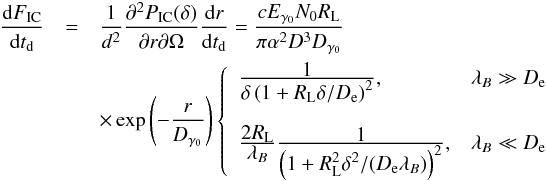$\begin{array}{ccc}\frac{\mathrm{d}{\mathit{F}}_{\mathrm{IC}}}{\mathrm{d}{\mathit{t}}_{\mathrm{d}}}& \mathrm{=}& \frac{\mathrm{1}}{{\mathit{d}}^{\mathrm{2}}}\frac{{\mathit{\partial }}^{\mathrm{2}}{\mathit{P}}_{\mathrm{IC}}\mathrm{\left(}\mathit{\delta }\mathrm{\right)}}{\mathit{\partial r\partial }\mathrm{\Omega }}\frac{\mathrm{d}\mathit{r}}{\mathrm{d}{\mathit{t}}_{\mathrm{d}}}\mathrm{=}\frac{\mathit{c}{\mathit{E}}_{{\mathit{\gamma }}_{\mathrm{0}}}{\mathit{N}}_{\mathrm{0}}{\mathit{R}}_{\mathrm{L}}}{\mathit{\pi }{\mathit{\alpha }}^{\mathrm{2}}{\mathit{D}}^{\mathrm{3}}{\mathit{D}}_{{\mathit{\gamma }}_{\mathrm{0}}}}\\ & & \mathrm{\times }\exp \left(\mathrm{-}\frac{\mathit{r}}{{\mathit{D}}_{{\mathit{\gamma }}_{\mathrm{0}}}}\right)\{\begin{array}{c}\\ & \\ & \\ & \end{array}\end{array}$(19)where r and δ = α + 2ct_d/Dα are expressed as functions of t_d.

Jet opening angle effects – The light curve of cascade emission from a jet of finite opening angle aligned with the line of sight can be obtained by summation of the light curves of all the beams forming the jet, i.e. via integration over the angle of the beam with respect to the line of sight α: 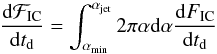$\frac{\mathrm{d}{\mathrm{ℱ}}_{\mathrm{IC}}}{\mathrm{d}{\mathit{t}}_{\mathrm{d}}}\mathrm{=}{\mathrm{\int }}_{{\mathit{\alpha }}_{\min }}^{{\mathit{\alpha }}_{\mathrm{jet}}}\mathrm{2}\mathit{\pi \alpha }\mathrm{d}\mathit{\alpha }\frac{\mathrm{d}{\mathit{F}}_{\mathrm{IC}}}{\mathrm{d}{\mathit{t}}_{\mathrm{d}}}$(20)where α_jet is the jet opening angle and α_min is found from the condition D/sinδ = D_γ0/sinα_min, which gives 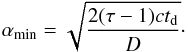${\mathit{\alpha }}_{\min }\mathrm{=}\sqrt{\frac{\mathrm{2}\mathrm{(}\mathit{\tau }\mathrm{-}\mathrm{1}\mathrm{)}\mathit{c}{\mathit{t}}_{\mathrm{d}}}{\mathit{D}}}\mathrm{·}$(21)Substituting the expression for dF_IC/dt_d (19) into (20) and taking the integral one finds at the limit of small t_d: 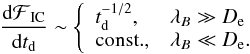$\frac{{\mathrm{dℱ}}_{\mathrm{IC}}}{\mathrm{d}{\mathit{t}}_{\mathrm{d}}}\mathrm{~}\{\begin{array}{c}\\ {\mathit{t}}_{\mathrm{d}}^{\mathrm{-}\mathrm{1}\mathit{/}\mathrm{2}}\mathit{,}& {\mathit{\lambda }}_{\mathit{B}}\mathrm{\gg }{\mathit{D}}_{\mathrm{e}}\\ \mathrm{const}\mathit{.}\mathit{,}& {\mathit{\lambda }}_{\mathit{B}}\mathrm{\ll }{\mathit{D}}_{\mathrm{e}}\mathit{.}\end{array}$(22)The slope of the cascade emission light curve depends on the relation between the IGMF correlation length and electron cooling distance. This fact can be used for the measurement of λ_B. At a fixed cascade photon energy, measurement of a flat cascade emission light curve would impose an upper bound on the IGMF correlation length, λ_B ≪ D_e. For the opposite case, a lower bound on λ_B would be set. If λ_B is larger than the IC cooling distance of the highest energy electrons, but shorter than the cooling distance of the lowest energy electrons contributing to the cascade γ-ray emission detectable by a γ-ray telescope, one expects to find a change in the slope of the cascade emission light curve at the energy E_γ,br where D_e ~ λ_B. In this case, measurement of the break energy E_γ,br would provide a measurement of the IGMF correlation length, given by Eq. (17). The range of length scales probable by this method is therefore dictated by the dynamic energy range of the instrument. For the example case of Fermi LAT, with a dynamic range of approximately 4 decades (20 MeV to 300 GeV Atwood et al. 2009), the corresponding coherence scale range probable by this method is 10  kpc ≲ λ_B ≲ 1 Mpc.

4. Verification with Monte Carlo simulation

Since relations (16) and (22) have been obtained using a simplified two-generation model, we here compare these results against those obtained with a complete multi-generation numerical description. Using the Monte Carlo simulation described in Taylor et al. (2011) in which the full cascade development is carried out and the spatial deflection of the electrons tracked a comparison of the two-generation results was carried out.

Adopting a delta-type injection spectrum with dN/dE_γ = δ(10¹³  eV), for a blazar redshift of z = 0.13, we compare in Figs. 2 and 3 the Monte Carlo obtained with expressions (16) and (22). Such comparisons confirm that the simplified analytic expressions obtained can indeed provide reasonably accurate descriptions of these distributions, particularly in the asymptotic regions. However, we do note that some degree of divergence is found in the intermediate region between the asymptotic zones for the small correlation length case (L_B/D_e ≪ 1).

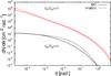Fig. 2 Angular profile of the arriving γ-ray flux following a flaring episode obstained with both Monte Carlo and analytic (Eq. (16)) methods. The angles shown are measured relative to the center of the blazar. For this plot, the angular profile of 1−3 GeV photons in a cascade from a source at z = 0.13 for a 10-15 G IGMF with coherence lengths 10 kpc (black lines) and 10 Mpc (red lines) are shown.

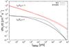Fig. 3 Time-delay in the arriving γ-ray flux following a flaring episode obstained with both Monte Carlo and analytic (Eq. (22)) methods. The time’s shown are measured relative to the straight line (SO in Fig. 1) arrival time. For this plot, the time-delay of 1−3 GeV photons in a cascade from a source at z = 0.13 for a 10-15 G IGMF with coherence lengths 10 kpc (black lines) and 10 Mpc (red lines) are shown.

5. Conclusion

Present generation γ-ray observational results have recently been used to provide challenging new bounds on the IGMF strength. The coherence length for this field, however, remains largely unconstrained. We here consider what handle future γ-ray observations may be able to provide with regards a measurement of both the IGMF strength and its coherence length. We show that measuring either the initial slope of the time delayed emission or the slope of the surface brightness profile of extended emission can be used to provide a measure of the IGMF correlation length.

Through the application of a simplified analytic two-generation model we describe two possible methods for probing this coherence length. Though both of these methods are potentially viable, the employment of the first of these methods would require considerable improvement in angular resolution above that achieved by present day γ-ray telescopes. The second of the methods put forward, however, does have the potential to be applied using forthcoming γ-ray observational data. A subsequent comparison of the two-generation model results with those obtained using the full Monte Carlo description confirms that this signature is still expected to survive once the full cascade physical description is added back into the picture.

References

All Figures

	Fig. 1 Geometry of cascade emission from a blazar jet SJ misaligned with the line of sight SO.
In the text

Fig. 2 Angular profile of the arriving γ-ray flux following a flaring episode obstained with both Monte Carlo and analytic (Eq. (16)) methods. The angles shown are measured relative to the center of the blazar. For this plot, the angular profile of 1−3 GeV photons in a cascade from a source at z = 0.13 for a 10-15 G IGMF with coherence lengths 10 kpc (black lines) and 10 Mpc (red lines) are shown.

In the text

Fig. 3 Time-delay in the arriving γ-ray flux following a flaring episode obstained with both Monte Carlo and analytic (Eq. (22)) methods. The time’s shown are measured relative to the straight line (SO in Fig. 1) arrival time. For this plot, the time-delay of 1−3 GeV photons in a cascade from a source at z = 0.13 for a 10-15 G IGMF with coherence lengths 10 kpc (black lines) and 10 Mpc (red lines) are shown.

In the text

References

- Aharonian, F. A., Coppi, P. S., & Voelk, H. J. 1994, ApJ, 423, L5 [NASA ADS] [CrossRef] [Google Scholar]
- Atwood, W. B., Abdo, A. A., Ackermann, M., et al. 2009, ApJ, 697, 1071 [NASA ADS] [CrossRef] [Google Scholar]
- Banerjee, R., & Jedamzik, K. 2004, Phys. Rev. D, 70, 3003 [NASA ADS] [Google Scholar]
- Bertone, S., Vogt, C., & Enßlin, T. 2006, MNRAS, 370, 319 [NASA ADS] [Google Scholar]
- Broderick, A. E., Chang, P., & Pfrommer, C. 2012, ApJ, 752, 22 [NASA ADS] [CrossRef] [Google Scholar]
- Dermer, C. D., Cavadini, M., Razzaque, S., et al. 2011, ApJ, 733, L21 [NASA ADS] [CrossRef] [Google Scholar]
- Dolag, K., Kachelriess, M., Ostapchenko, S., & Tomàs, R. 2011, ApJ, 727, L4 [NASA ADS] [CrossRef] [Google Scholar]
- Franceschini, A., Rodighiero, G., & Vaccari, M. 2008, A&A, 487, 837 [NASA ADS] [CrossRef] [EDP Sciences] [Google Scholar]
- Hogan, C. J. 1983, Phys. Rev. Lett., 51, 1488 [Google Scholar]
- Ichiki, K., Inoue, S., & Takahashi, K. 2008, ApJ, 682, 127 [NASA ADS] [CrossRef] [Google Scholar]
- Miniati, F., & Elyiv, A. 2012 [arXiv:1208.1761] [Google Scholar]
- Murase, K., Takahashi, K., Inoue, S., Ichiki, K., & Nagataki, S. 2008, ApJ, 686, L67 [NASA ADS] [CrossRef] [Google Scholar]
- Neronov, A., & Semikoz, D. V. 2007, JETP Lett., 85, 473 [CrossRef] [Google Scholar]
- Neronov, A., & Vovk, I. 2010, Science, 328, 73 [NASA ADS] [CrossRef] [PubMed] [Google Scholar]
- Orr, M. R., Krennrich, F., & Dwek, E. 2011, ApJ, 733, 77 [NASA ADS] [CrossRef] [Google Scholar]
- Plaga, R. 1995, Nature, 374, 430 [NASA ADS] [CrossRef] [Google Scholar]
- Quashnock, J. M., Loeb, A., & Spergel, D. N. 1989, ApJ, 344, L49 [NASA ADS] [CrossRef] [Google Scholar]
- Schlickeiser, R., Ibscher, D., & Supsar, M. 2012, ApJ, 758, 102 [NASA ADS] [CrossRef] [Google Scholar]
- Sigl, G., Olinto, A. V., & Jedamzik, K. 1997, Phys. Rev. D, 55, 4582 [Google Scholar]
- Takahashi, K., Murase, K., Ichiki, K., Inoue, S., & Nagataki, S. 2008, ApJ, 687, L5 [NASA ADS] [CrossRef] [Google Scholar]
- Tavecchio, F., Ghisellini, G., Bonnoli, G., & Foschini, L. 2011, MNRAS, 414, 3566 [NASA ADS] [CrossRef] [Google Scholar]
- Taylor, A. M., Vovk, I., & Neronov, A. 2011, A&A, 529, A144 [NASA ADS] [CrossRef] [EDP Sciences] [Google Scholar]
- Vachaspati, T. 1991, Phys. Lett. B, 265, 258 [NASA ADS] [CrossRef] [Google Scholar]
- Vovk, I., Taylor, A. M., Semikoz, D., & Neronov, A. 2012, ApJ, 747, L14 [NASA ADS] [CrossRef] [Google Scholar]