| Issue |
A&A
Volume 558, October 2013
|
|
|---|---|---|
| Article Number | A104 | |
| Number of page(s) | 8 | |
| Section | Planets and planetary systems | |
| DOI | https://doi.org/10.1051/0004-6361/201322221 | |
| Published online | 14 October 2013 | |
Compact YORP formulation and stability analysis
Department of Mathematics, Tampere University of Technology, PO Box 553, 33101 Tampere, Finland
e-mail: This email address is being protected from spambots. You need JavaScript enabled to view it.
Received: 6 July 2013
Accepted: 3 September 2013
Abstract
We present a concise analytical formulation of the YORP effect, with exact formulae for torques on convex bodies and motion-averaged components applicable to any shapes. We analyze the main features of the secular torques for zero and nonzero thermal inertia that are function series dependent on only a few coefficients. Using these, we investigate the stability of the YORP effect against shape perturbations with analytical and numerical estimates. We define a quantity describing the YORP capacity of any shape, and estimate YORP stability with it.
Key words: methods: analytical / methods: numerical / radiation mechanisms: thermal / minor planets, asteroids: general / minor planets, asteroids: individual: (1862) Apollo / minor planets, asteroids: individual: (3103) Eger
© ESO, 2013
1. Introduction
The effect of sunlight on the dynamics of small asteroids is now known to be considerable over long time spans. The anisotropic reflection and thermal re-emission of solar photons is essentially equivalent to a large number of small rocket engines distributed on the surface of an asteroid. Thus the dynamical mechanisms are usually divided into two categories: the net propulsion force changing the orbital motion (the Yarkovsky effect), and the net torque affecting the rotational dynamics (the Yarkovsky-O’Keefe-Radzievskii-Paddack or YORP effect). Both have been observed directly (Chesley 2003; Kaasalainen et al. 2007; Lowry et al. 2007; Ďurech et al. 2008, 2012), and there is clear indirect evidence of their long-term role in the evolution of asteroid orbits and spin states (Bottke et al. 2001; Vokrouhlický et al. 2003, 2006).
The analytical modeling of the YORP torques, or any other illumination-dependent functions, on general shapes is constrained by the concept of insolation: in which geometries is a surface patch visible? For convex bodies insolation is trivial, and they are the only ones for which exact analytical torques are possible. Various semianalytical approaches have developed small nonconvex perturbations while neglecting numerical ray-tracing within some perturbation size (e.g., Breiter & Michalska 2008; Nesvorný & Vokrouhlický 2007, 2008a; hereafter NV07 and NV08). Unfortunately, the shadowing error cannot be estimated in terms of the perturbation parameter, so no validity regime can be established for such approximations even when the perturbation is very small.
We present the fundamentals of the YORP effect and its stability and symmetry properties in a conceptually and technically simple analytical and exact formulation. For example, it is easy to identify the enigmatic YORP instability with the “trash coefficients” of a Laplace series, and to show that, while quadrant-symmetric bodies have no secular YORP torques for zero thermal inertia (K = 0), they acquire a nonvanishing component for K ≠ 0. Breiter et al. (2011; hereafter BRV11) arrive at some of the results of Sect. 3 (K = 0) by a different context and approach. We provide easy-to-use formulae directly applicable to typical body representations such as polyhedra. The motion-averaged formulation pertains to any shapes.
We discuss the basic concepts and functions in Sect. 2. The cases of zero and nonzero thermal inertia are studied in, respectively, Sects. 3 and 4. The YORP effect can be very sensitive to the details of the shape and other physical characteristics of the body (Statler 2009; Rozitis & Green 2012), so we discuss YORP stability in Sect. 5. We sum up in Sect. 6, and numerical formulae for convex polyhedral shape representations are presented in an appendix.
2. Problem setup and definitions
Let the direction of the illumination source in a coordinate system fixed to the target body (the z-axis coinciding with the rotation axis) be denoted by ω ∈ S2. Here entities on the unit sphere S2, defined by two direction angles, are identified with unit vectors in R3. Thus, e.g., the outward unit normal vector η ∈ S2 is given by η = η(ϑ,ψ) (with ϑ measured from the pole), 0 ≤ ϑ ≤ π, 0 ≤ ϑ < 2π; i.e.,  (1)Likewise, ω = ω(θ,ϕ) (the subsolar coordinates). The position of the asteroid around the Sun in the orbital frame is given by λ, 0 ≤ λ < 2π, and the tilt (obliquity) of the rotation axis from the orbital pole is denoted by ϵ, 0 ≤ ϵ ≤ π. The orbital frame and the pole direction of the asteroid are chosen such that
  (2)For clarity, we assume a circular orbit around the Sun. Ellipticity is straightforward to include as described in NV07 and NV08, and in any case the modifications due to ellipticity are only of order
  for eccentricity e (NV07). Denoting the rotation angle of the asteroid around its axis by ϕ′: = Ωt, the transformation of a vector v from the orbital frame to the body frame reads
  (3)where Ri are the usal rotation matrices for z- and y-axes (Kaasalainen & Lamberg 2006). The transformations to an oblique frame aligned with the rotation axis but not rotating with the asteroid are
  (4)The oblique frame is needed in computing the torque component that changes the obliquity of the spin axis. We assume here that λ remains virtually constant during 2π/Ω.
2.1. Characteristic torque function
The thermal YORP torque by emitted photons is given by (NV07, NV08)  (5)where the integral is taken over the whole surface of the body ℬ (of arbitrary shape and topology), T is the surface temperature, γ is the product of the emissivity of the material in thermal wavelengths and the Stefan-Boltzmann constant, and vc is the speed of light. (As shown in Nesvorný & Vokrouhlický 2008b, the torque due to absorbed photons vanishes identically when averaged over orbit revolution and body rotation.)
We define the characteristic torque function  of a body as the three-dimensional vector
  (6)where ξ is any two-dimensional parametrization of the location on the surface. For a convex body,
  (7)where G(η) is the curvature function, so we consider on S2:
  (8)(cf. BRV11). For asteroids, G(η) is typically an initial product from observational data, and x(η) is derived from it as the solution of the Minkowski problem (usually as a convex polyhedron; Kaasalainen et al. 1992, 2006).
Expanding as a Laplace series, we have  (9)Here we ignore the customary normalization constants of the spherical harmonics
  as they can always be introduced as normalization factors when actually taking orthogonality integrals, so
  . Written explicitly as a real-valued function,
 ![Mathematical equation: \begin{equation} {\mathcal T}_i(\eta)=\sum_{l\ge 0}\sum_{m=0}^l P_l^m(\vartheta,\psi) \left[T_{lm}^{i,\cos}\cos(m\psi)+T_{lm}^{i,\sin}\sin(m\psi)\right]. \label{treal} \end{equation}](/articles/aa/full_html/2013/10/aa22221-13/aa22221-13-eq43.png) (10)The possible symmetries of
(10)The possible symmetries of  are evident in Tlm. For example, geometric inspection shows that if the body is symmetric about a line in the xy-plane, Tl0 ≡ 0. If the body is quadrant-symmetric (e.g., an ellipsoid), the Fourier terms are
  ,
,  with m odd, while
  with m even. The coefficients Tlm are readily calculated with the formulae in the appendix.
3. YORP torque and its components for K = 0
When there is no thermal inertia; i.e., the thermal conductivity K = 0, the absorbed flux is emitted immediately. Denoting  (11)the immediate emission means that, for a surface patch dS,
  (12)where A is the surface albedo and Fo the incoming solar flux. Thus we have, denoting the illuminated portion of the surface by A+ and writing the convex version explicitly,
  (13)where Q has the physical dimension of pressure:
  (14)The effect of albedo variegation A(η) on the surface can be absorbed in
  by replacing G(η) with [1 − A(η)] G(η) in (8) and defining Q = −2F0/3vc.
The YORP torque in the body frame is now obtained in the same way as the opposition brightness for convex bodies (Kaasalainen et al. 1992; now we just have the coefficients of a three-dimensional Laplace series). Thus we have the fundamental result for the YORP torque τ:  (15)where, for convex bodies, tlm = 2πkl Tlm, and
  (16)Other values of l are not of interest as the odd ones drop out for all shapes in averaging (see below), and T00 vanishes identically due to Gauss’ theorem.
As pointed out in BRV11, the torque τ for any shape, computed on a grid of (θ,ϕ) by ray-tracing, can, of course, be expressed as a Laplace series by using, e.g., Lebedev-Laikov quadratures (Kaasalainen et al. 2012). The coefficients tlm can be used in the following analytical motion-averaged formulae that no longer require convexity, although the relevant tlm tend to be unstable, as discussed in Sect. 5.
3.1. Rotation speed
Averaging over one rotation, we have  (17)The secular torque
  is obtained by averaging over λ:
  (18)where
  (19)Thus Il = 0 for odd l, and for even l we obtain, using the recursion relations of Legendre polynomials,
  (20)where
  (21)Our final expression for is now simply
 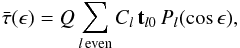 (22)which manifestly vanishes for azimuthally symmetric bodies due to the structure of Tlm discussed above. The torque component that alters the rotation speed of the body is the z-component
  given by the coefficients
  . If the series is dominated by
  , this component essentially vanishes at the roots of P2(cosϵ), i.e., at ϵ ≈ 55° and ϵ ≈ 125° (cf. NV07).
Shape-related phenomena that are apparent instabilities are obvious from this result. These are actually critical phenomena on a shape close to tl0 = 0. Consider, say, a pointed local feature on an otherwise symmetric (e.g., ellipsoidal) body at ϑ = π/2, ψ = δ > 0. This feature produces a small  . On the other hand, a similar arrangement symmetric about the x-axis, with the center of the feature at ψ = −δ, yields exactly
  . Note that δ can be arbitrarily small. One can view this as a minuscule shift of a local feature on the body: practically invisible to the eye, yet the YORP torque changes its sign. This is an analogue of the numerical “boulder shift” phenomenon discussed in Statler (2009).
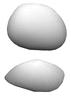 |
Fig. 1 Convex model shapes of asteroids Psyche (top) and Apollo (bottom). |
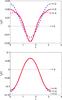 |
Fig. 2 Secular YORP torque |
As an example, we evaluated from Eq. (22) for the convex shapes shown in Fig. 1. In Fig. 2, the various linestyles for different numbers of  -terms show the rapid convergence of the series. Note that, throughout this paper, we only analyze the shapes of asteroids, so we do not take sizes and masses into account (and set Q = 1). Thus the scale of is arbitrary.
3.2. Obliquity
The torque component τϵ that alters the obliquity of the rotation axis is given by the rotational transformation of Eq. (4): ![Mathematical equation: \begin{equation} \tau_\epsilon=\left[{\bf R}_z(-\varphi')\tau\right]_1=\tau_1\cos\varphi'- \tau_2\sin\varphi'.\label{tauetrans} \end{equation}](/articles/aa/full_html/2013/10/aa22221-13/aa22221-13-eq103.png) (23)In the same oblique coordinate frame (i.e., the z-axis is aligned with the rotation axis and the x-component of τ is τϵ), the direction of the Sun is given by
(23)In the same oblique coordinate frame (i.e., the z-axis is aligned with the rotation axis and the x-component of τ is τϵ), the direction of the Sun is given by  (24)Thus
  (25)and substituting this to (23) yields
  (26)From Eq. (24) we find that
  (27)so, substituting τ1 and τ2 from Eq. (15), using real-valued tlm, and averaging over ϕ with Eq. (25),
 ![Mathematical equation: \begin{eqnarray} \tau_\epsilon(\lambda,\epsilon)&=&\frac{Q}{2}\sum_l P_l^1(\cos\lambda\sin\epsilon)\label{tauephi} \left[\cos\varphi_s\left(t_{l1}^{1,\cos}+t_{l1}^{2,\sin}\right)\right.\\[2mm] \nonumber &&\left.+~\sin\varphi_s\left(t_{l1}^{1,\sin}-t_{l1}^{2,\cos}\right)\right], \end{eqnarray}](/articles/aa/full_html/2013/10/aa22221-13/aa22221-13-eq112.png) (28)and averaging over λ, we obtain
(28)and averaging over λ, we obtain 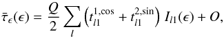 (29)where
 ![Mathematical equation: \begin{eqnarray} I_{l1}(\epsilon)&=&\frac{1}{\pi}\int_0^{\pi}P_l^1(\cos\lambda\sin\epsilon) \frac{\cos\epsilon\cos\lambda}{\sqrt{1-\sin^2\epsilon\cos^2\lambda}}\,{\rm d}\lambda \\[2mm] \nonumber &=&\frac{1}{\pi}\frac{\cos\epsilon}{\sin\epsilon} \int_{-\sin\epsilon}^{\sin\epsilon} \frac{x\,P_l^1(x)}{\sqrt{1-x^2}}\frac{{\rm d}x}{\sqrt{\sin^2\epsilon-x^2}}, \end{eqnarray}](/articles/aa/full_html/2013/10/aa22221-13/aa22221-13-eq114.png) (30)so Il1 = 0 for odd l, and O denotes the sinϕs-terms that vanish because of the parity of
(30)so Il1 = 0 for odd l, and O denotes the sinϕs-terms that vanish because of the parity of  and the requirement of an antisymmetric τϵ:
  . Computing the integral in the same way as with , we have
  (31)Owing to the structure of Tlm, this vanishes for quadrant-symmetric bodies. In BRV11, Eqs. (29), (C14), and (C15) are alternative versions of Eqs. (15), (22), and (31) here.
4. Nonzero thermal conductivity
Let us define the insolation factor ins(μ,ξ) as ins(μ,ξ) = μ if the point ξ on the surface is illuminated, and otherwise ins(μ,ξ) = 0. For constant λ and ϵ, ins(μ,ξ) is obviously a cyclic function of ϕ′, so it can be expanded as a Fourier series:  (32)The coefficients dn(ξ,λ,ϵ) can always be readily computed, analytically for convex bodies and by ray-tracing and FFT for others. In this analysis, however, we do not need their actual values; it is sufficient to know that they exist and fully define ins(μ,ξ) (even when it is discontinuous due to shadowing by nonconvexities).
Writing τ by using ins(μ,ξ) instead of A+, we have, for K = 0,  (33)When averaging over ϕ′, the only contributing term is the one with n = 0.
For K ≠ 0, the heat diffusion equation  (34)where ρ is the density of the material, cp is the specific heat capacity, and the vertical direction ξ is aligned with η, can be solved with suitable physical approximations, boundary conditions, and a periodic ansatz of the form (32) (see NV08). With damping factors Ψn and phase lags Δφn defined by
  (35)where
  (36)an approximate solution is
  (37)so
  (38)Again, averaging over ϕ′ retains only the n = 0 -contribution, and Ψ0 = 1, Δφ0 = 0, so the result is exactly the same as with K = 0. This shows that K has no influence on the rotation-averaged τ.
4.1. Obliquity torque
Using the rotation-transform Eq. (23) for τϵ together with the real-valued Fourier series in (32), we have, from Eqs. (23) and (33), ![Mathematical equation: \begin{eqnarray} \tau_\epsilon(\lambda,\epsilon,\varphi') &=&Q\sum_n \left[\cos n\varphi'\cos\varphi' \int_{\mathcal B}{\mathcal T}_1(\xi)a_n(\xi,\lambda,\epsilon)\,{\rm d}S\right.\\\nonumber &&\left.-\,\sin n\varphi'\sin\varphi'\int_{\mathcal B} {\mathcal T}_2(\xi)b_n(\xi,\lambda,\epsilon) \,{\rm d}S\right]+O, \end{eqnarray}](/articles/aa/full_html/2013/10/aa22221-13/aa22221-13-eq143.png) (39)where O denotes cross-terms that vanish in averaging over ϕ′. Upon this averaging, we obtain an expression for K = 0 (Δφn = 0) in the Fourier-series representation:
(39)where O denotes cross-terms that vanish in averaging over ϕ′. Upon this averaging, we obtain an expression for K = 0 (Δφn = 0) in the Fourier-series representation: ![Mathematical equation: \begin{equation} \tau_\epsilon(\lambda,\epsilon)=\frac{Q}{2} \int_{\mathcal B}\left[{\mathcal T}_1(\xi)a_1(\xi,\lambda,\epsilon) -{\mathcal T}_2(\xi)b_1(\xi,\lambda,\epsilon)\right]\,{\rm d}S, \end{equation}](/articles/aa/full_html/2013/10/aa22221-13/aa22221-13-eq145.png) (40)which is thus equivalent to the ϕ-averaged τϵ of Eq. (28), when assuming constant λ during the averaging.
(40)which is thus equivalent to the ϕ-averaged τϵ of Eq. (28), when assuming constant λ during the averaging.
Next we expand the above expression to K ≠ 0. With a real-valued Fourier series solution for T4, averaging τϵ(λ,ϵ,ϕ′) from Eq. (38) over ϕ′ yields ![Mathematical equation: \begin{eqnarray} \tau_\epsilon(\lambda,\epsilon)&=& \frac{Q}{2}\Psi_1\left[\cos\Delta\phi_1 \int_{\mathcal B}\left({\mathcal T}_1a_1-{\mathcal T}_2b_1\right)\,{\rm d}S\right.\\\nonumber &&-\,\left.\sin\Delta\phi_1 \int_{\mathcal B}\left({\mathcal T}_2a_1+{\mathcal T}_1b_1\right)\,{\rm d}S\right]. \end{eqnarray}](/articles/aa/full_html/2013/10/aa22221-13/aa22221-13-eq148.png) (41)In other words,
(41)In other words, ![Mathematical equation: \begin{equation} \tau_\epsilon(\lambda,\epsilon)=\Psi_1\left[\cos\Delta\phi_1\tau_\epsilon\left( \tau\vert_{\Delta\phi\,=\,0}\right)+\sin\Delta\phi_1\tau_\epsilon\left( \tau\vert_{\Delta\phi\,=\,\frac{\pi}{2}}\right)\right], \end{equation}](/articles/aa/full_html/2013/10/aa22221-13/aa22221-13-eq149.png) (42)where τϵ(τ | Δφ = α) denotes τϵ(λ,ϵ) computed with a phase-lagged τ evaluated at ϕ′ − α instead of ϕ′; a phase lag of α = π/2 changes a1 → − b1 and b1 → a1 in the Fourier series. Using ϕ → ϕs − (ϕ′ − π/2), i.e., ϕ → ϕ + π/2, in the fundamental Eq. (15) for τ when averaging over ϕ and λ, we obtain our final result:
(42)where τϵ(τ | Δφ = α) denotes τϵ(λ,ϵ) computed with a phase-lagged τ evaluated at ϕ′ − α instead of ϕ′; a phase lag of α = π/2 changes a1 → − b1 and b1 → a1 in the Fourier series. Using ϕ → ϕs − (ϕ′ − π/2), i.e., ϕ → ϕ + π/2, in the fundamental Eq. (15) for τ when averaging over ϕ and λ, we obtain our final result: ![Mathematical equation: \begin{eqnarray} \bar\tau_\epsilon(\epsilon)&=&\frac{Q}{2}\Psi_1\sum_{l\,\mathrm{even}} C_l\,P_l^1(\cos\epsilon)\,\left[\cos\Delta\phi_1\label{Kno0} \left(t_{l1}^{1,{\rm cos}}+t_{l1}^{2,{\rm sin}}\right)\right.\\\nonumber &&\left.-\,\sin\Delta\phi_1\left(t_{l1}^{1,{\rm sin}}+t_{l1}^{2,{\rm cos}}\right)\right]. \end{eqnarray}](/articles/aa/full_html/2013/10/aa22221-13/aa22221-13-eq158.png) (43)This means that, at large values of KΩ, the YORP torque
(43)This means that, at large values of KΩ, the YORP torque  acquires a significant component that does not vanish even for ellipsoids, for example.
5. YORP stability
If we consider the coefficients tlm in the basic torque Eq. (15), we can see that those determining the secular torques are precisely the ones that are usually vanishingly small compared to the momentary torque level. For example, an elongated ellipsoid produces large nonsecular torques, while the secular ones vanish. Thus even a small change in the shape of a body inevitably alters the secular torques with a much larger relative factor. If tlm are determined numerically from the momentary torques with various illumination directions on S2, the secular “trash coefficients” are easily affected by their errors, and can even be drowned in the numerical noise. This also helps to understand YORP instability as a fundamental and inevitable fact.
The analytical expressions in Sects. 3 and 4 provide a general set of convenient basis functions for the presentation of numerical YORP computations in a compact form. A robust approach for general shapes, especially those far from convex surfaces, is to compute the secular torques numerically with ray-tracing and averaging, and then fit series in Pl(cosϵ) or  , l even, to them. This one-dimensional procedure is more stable than the determination of the Laplace series of Eq. (15). One way to compute torques with K ≠ 0 is to evaluate the cases with emission phase lags of 0 and π/2 and then form their superposition by modulating with the phase lag Δφ1 to conform with Eq. (43).
Many asteroids are well approximated by convex shapes (up to some level of resolution), so if two shapes differ only slightly, how different are their YORP properties? This question concerns not only the validity regime of an approximation, but the general stability properties of the YORP effect as well.
In this context, it is useful to normalize the YORP torques to be size-invariant, pertaining only to the shape of the object. Since the dimension of the torque integrand is that of volume, we define the dimensionless YORP capacity of a shape as the maximal average torque per unit volume and unit flux pressure (or torque when the volume V and the pressure are scaled to unity): 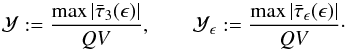 (44)The YORP capacity
  thus describes the amplitude of the -curve of the unity-scaled case. For most convex shapes, is fast to evaluate directly from
  with Eq. (22), and
  similarly with Eqs. (31) or (43). Conversely, given for any shape, one can quickly compute the actual maximal torque by multiplying by QV.
To establish a scale for , consider a “propeller” shape consisting of two identical vertically symmetric wedges attached to each other inversion-symmetrically (Fig. 3). The maximal YORP torque is attained at ϵ = 0,π. The cross-section of a wedge is an isosceles triangle with height h and width w, and the length of a wedge is l. If we assume a long and thin body with h/l ≪ 1 (and w/l ≪ 1), we can neglect the torques from the ends of the wedges and terms of order (h/l)2 and higher, so 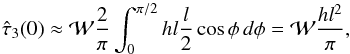 (45)where the efficiency factor
  of the sharpness of the wedge is
 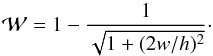 (46)Thus, with V = hwl and estimating from
  ,
, 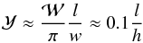 (47)for a flattening ratio w/h = 3/2 realistic for an asteroid. An infinitely long and thin body yields
  , so there is no upper bound for the YORP capacity in principle. For realistic shapes l/h ~ 1, we can estimate an upper bound
  .
.
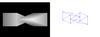 |
Fig. 3 Wedge-propeller shape strongly prone to the rotational YORP torque, shown as a solid object and as a wire frame. |
Any suitably asymmetric, infinitely long and thin shape yields , so there is no unique answer to the question “what is the most YORP-prone shape”, nor is there a unique solution to the problem “what is the most YORP-efficient realistic asteroid shape” since the term “realistic” can be defined in a number of ways. The wedge-propeller shape is more or less the optimal one for YORP-efficiency as it portrays the best “windmill asymmetry” profile.
To study the stability problem, let us estimate an upper bound for the change  due to the perturbation Δx that affects the characteristic torque function:
  (48)Consider, e.g., the perturbed unit sphere, so that
  (the estimate is essentially similar for all convex bodies, but we choose the sphere for a simple example). Thus
 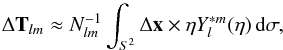 (49)and we can approximate, with a perturbation Δx = f(η), where f(η) is a Laplace series such that x + Δx is convex and ⟨ ∥ f ∥ ⟩ η = δ,
 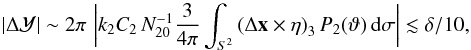 (50)where the upper bound for the integral is estimated by applying the Legendre recursion formulae to the products with the components of η and using the orthogonality integral. A perturbation of δ = 0.1 can thus produce a change
  roughly a tenth of the wedge propeller’s above; in practice, the change is usually smaller than this.
When estimating the change of YORP properties due to perturbations, we only consider the change  in amplitude. Indeed, taking the leading Legendre term as in Eq. (50) implies that the changes in the phase (the value of ϵ at the maximum) and the shape of are, for small shape perturbations, negligible compared to the amplitude change.
In addition to by surface fluctuations of a given size (that typically describe the convexity/nonconvexity or resolution difference between two shape models), we can consider a couple of other mechanisms for comparison: i) the “boulder effect” and ii) the effect of scale-invariant surface roughness. If we attach the wedge above to the surface of a sphere of radius r, and fix h = w = l = δr, we have  , so adding a boulder of size r/10 changes by
  . If we consider a special arrangement of infinitesimal wedges on the surface, all pointing in an ordered way such that l/h = c and h2 → dσ and hl → c dσ, we obtain an upper bound
 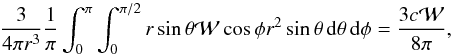 (51)so a moderate surface roughness c ≈ 0.1 yields
  . In principle, one can coat a sphere such that it looks smooth and yet is, paradoxically, quite prone to YORP. The upper bound cannot be reached by a realistic unordered surface structure, but
  is plausible. Thus, taking a single large boulder or the unseen small-scale surface structure into account on a small asteroid can change up to
  .
.
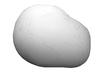 |
Fig. 4 Nonconvex perturbation based on the model shape of the asteroid Psyche in Fig. 1. Here the value of the YORP capacity |

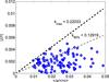 |
Fig. 5 Plot of ⟨ Δr ⟩ / ⟨ r ⟩ versus |
Given the analytical scale estimates of and  above, are there YORP-stable asteroid shapes in reality? We measured the YORP values and their perturbations for some targets, when the shape perturbations were global nonconvex radius fluctuations Δr of varying magnitude (by low-order Laplace series), and was computed by ray-tracing. A sample perturbation is shown in Fig. 4. For each shape and sequence of perturbations
  , one can define an upper bound kmax such that
 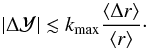 (52)To estimate this, we plotted ⟨ Δr ⟩ / ⟨ r ⟩ vs. for each shape; a sample case is shown in Fig. 5. A bounding line is approximately at kmax ≈ [0.1,0.2], consistent with the upper bound δ/10 estimated above. What is more, the slope kmax decreases as ⟨ Δr ⟩ / ⟨ r ⟩ grows ( may even saturate) so the linear upper bound estimate is only a rough approximation for small perturbations. For most shapes, kmax ~ 0.1 for a practical estimate. The estimate is not strict, nor can a shape perturbation be properly described by one figure ⟨ Δr ⟩ / ⟨ r ⟩ only.
The global perturbation scheme depicts the case of two alternative representations of the same body – for example, a lightcurve-based model and a radar-based one, or two versions of a model based on flyby data. If the model error ⟨ Δr ⟩ / ⟨ r ⟩ remains small, we can estimate shapes with  (such as Apollo) to be reasonably YORP-stable against global model errors in the sense of the relative YORP error
  . Any instability in this error is caused by the inevitable smallness of rather than the size of
  .
.
Another interesting case is the “boulder effect”; it represents a local model error, or an actual local change of the shape due to some physical perturbation. We made random local changes to bodies and measured the YORP change; a scatter plot similar to that of global perturbations is shown in Fig. 6. In this case, most of the YORP changes are negligible, while some jump to  . As in the analytical estimate above, the relative YORP changes remain well bounded for shapes with (such as the plotted case of Apollo), while shapes with
  are no longer YORP-stable against local shape perturbations.
In Table 1, we show sample values of for a number of asteroid shapes (obtained from the DAMIT website). Note again that is size-independent, and the samples represent typical asteroid shapes rather than estimates for the actual bodies, many of which are large and not affected by YORP.
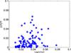 |
Fig. 6 Plot of ⟨ Δr ⟩ / ⟨ r ⟩ versus |

List of the YORP capacity  of different asteroid shapes.
To sum up the analytical and numerical stability estimates above as a rough order-of-magnitude classification scheme, we can define YORP stability classes as  (53)where round(x) gives the integer closest to x, and the constant 1.8 was chosen to set the lower class limit to
  . Most asteroid shapes are in the regime n ≤ − 1; some reach n = 0, and mostly propeller-type shapes have n ≥ 1. Depending on the stability class, all the perturbation scenarios above can change from tens of percent to orders of magnitude for typical asteroid shapes in a quite natural manner. As a ballpark estimate, we could call shapes with n = 0 locally YORP-stable and globally semistable, while those with n = −1 are locally semistable and globally unstable. All shapes in the classes n < − 1 are YORP-unstable, and those in n ≥ 1 YORP-stable.
Most of the shapes in Table 1 are in n = −1; only “Massalia”, “Apollo”, “Geographos”, and “Eger” are in n = 0. For the last three of these more stable ones, the YORP effect has been observed directly from lightcurves (Kaasalainen et al. 2007; Ďurech et al. 2008, 2012). The stability estimate is consistent with the good correspondence between the computed and observed YORP acceleration for Apollo and Geographos. For Eger, the correspondence is not as good. The value of thus indicates that this is more due to its unknown sizable nonconvex features than the smaller-scale irregularities (the cited value is based on the adopted nonconvex shape solution; the convex one has an even higher  ). Indeed, Eger is notable for being one of the few asteroids for which lightcurves indicate strong nonconvexities (Ďurech & Kaasalainen 2003). Some main features can be sketched from photometric data (Ďurech et al. 2012), but the solution is not unique, which may cause the discrepancy between the expected and real YORP strengths.
As in the analytical estimates, the amplitude change  dominated our numerical perturbation cases. This means that, for most of the -curve, determines the stability class. However, when ϵ is close to the values at which vanishes (i.e., usually around ϵ ≈ 55° and ϵ ≈ 125°), the changes in the phase and shape of the curve induced by the shape perturbation are significant for the relative change in . Near these obliquities, all shapes are YORP-unstable.
6. Conclusions and discussion
We have presented a concise formalism for analyzing YORP-related quantities. Using the characteristic torque function of the body, defined by Eq. (8), one can readily write the general Eq. (15) for the YORP torque as well as its main secular components of interest: the one changing the rate of rotation and the one altering the obliquity. The motion-averaged results can be given for both zero (Eqs. (22), (31)) and nonzero (Eq. (43)) thermal inertia. Since the averaging integrals are analytical regardless of the shape, the formulae also provide a convenient set of basis functions for representing YORP computations of nonconvex shapes.
The YORP effect as such is stable in principle; i.e., a small change in the shape leads to a small change in the YORP capacity . What causes the unpredictability is the relative change  because most asteroids tend to have close to zero. Here we have derived a number of analytical and numerical estimates on YORP stability, and, based on these, surmise that most asteroids tend to be YORP-unstable, though some can reach a stable class. The stability class is determined by the YORP capacity : the larger the capacity, the better the relative YORP stability. For convex polyhedra, a simple approximation of is obtained from the P2-coefficient of :
 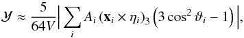 (54)where Ai, xi, and ηi are the area, centroid, and unit normal of a facet, and ϑi is the polar angle of the normal (see Appendix). This approximation can also be used directly for slightly nonconvex shapes to obtain a first estimate; for these, the sum over facets is almost similar to a convex case.
Here we have simplified the YORP business to the extreme at the expense of accuracy, but Eq. (54) provides some equational economy: with it (and its variants for other torques), we can approximate and and estimate the YORP stability of a body. For more strongly nonconvex shapes, one can construct the best-fit convex shape by, e.g., scaling the convex hull suitably (semianalytical generalizations of NV07 via a perturbation of this shape are also relatively straightforward, but they lose the conceptual simplicity with no certainty of better accuracy). If the fluctuations around this surface do not exceed, say, a tenth part of the radius, the analytical result is reasonably reliable if . For  , the accuracy of any YORP estimate (not just the types discussed here) is uncertain due to the instability. For
  , all YORP estimates are likely to be invalid, and only upper bounds can be given. The same applies to YORP estimates made near the obliquity at which the averaged net torque vanishes, regardless of .
An unstable class does not mean that all shape perturbations induce a large change in , but that suitable ones can do so. It would be interesting to explore the YORP stability properties in “shape space” by evaluating and for a large number of both convex and nonconvex shapes and their perturbations by craters and valleys. This would shed more light on the role of the YORP effect in the evolutionary history of asteroids. For example, a small asteroid with a low YORP capacity is likely to undergo a more stochastic YORP-affected spin evolution than one with a higher value of , since even small alterations of the shape may be significant for the YORP effect.
Acknowledgments
This work was supported by the Academy of Finland project “Modelling and applications of stochastic and regular surfaces in inverse problems”. We thank David Vokrouhlický for valuable comments that improved the manuscript.
References
- Bottke, W. F., Vokrouhlický, D., Broz, M., et al. 2001, Science, 294, 1693 [NASA ADS] [CrossRef] [PubMed] [Google Scholar]
- Breiter, S., & Michalska, H. 2008, MNRAS, 388, 927 [NASA ADS] [CrossRef] [Google Scholar]
- Breiter, S., Rozek, A., & Vokrouhlický, D. 2011, MNRAS, 417, 2478 (BRV11) [NASA ADS] [CrossRef] [Google Scholar]
- Chesley, S. R., Ostro, S. J., Vokrouhlický, D., et al. 2003, Science, 302, 1739 [NASA ADS] [CrossRef] [Google Scholar]
- Ďurech, J., & Kaasalainen, M. 2003, A&A 404, 709 [Google Scholar]
- Ďurech, J., Vokrouhlický, D., Kaasalainen, M., et al. 2008, A&A, 489, L25 [NASA ADS] [CrossRef] [EDP Sciences] [Google Scholar]
- Ďurech, J., Vokrouhlický, D., Baransky, A. R., et al. 2012, A&A, 547, A10 [NASA ADS] [CrossRef] [EDP Sciences] [Google Scholar]
- Kaasalainen, M., & Lamberg, L. 2006, Inverse Problems, 22, 749 [Google Scholar]
- Kaasalainen, M., Lamberg, L., Lumme, K., & Bowell, E. 1992, A&A, 259, 318 [NASA ADS] [Google Scholar]
- Kaasalainen, M., Ďurech, J., Warner, B., et al. 2007, Nature, 446, 420 [NASA ADS] [CrossRef] [PubMed] [Google Scholar]
- Kaasalainen, M., Lu, X., & Vänttinen, A. 2012, A&A, 539, A96 [NASA ADS] [CrossRef] [EDP Sciences] [Google Scholar]
- Lowry, S. C., Fitzsimmons, A., Pravec, P., et al. 2007, Science, 316, 272 [NASA ADS] [CrossRef] [PubMed] [Google Scholar]
- Nesvorný, D., & Vokrouhlický, D. 2007, ApJ, 134, 1750 (NV07) [Google Scholar]
- Nesvorný, D., & Vokrouhlický, D. 2008a, ApJ, 136, 291 (NV08) [Google Scholar]
- Nesvorný, D., & Vokrouhlický, D. 2008b, A&A, 480, 1 [NASA ADS] [CrossRef] [EDP Sciences] [Google Scholar]
- Rozitis, B., & Green, S. 2012, MNRAS, 423, 367 [NASA ADS] [CrossRef] [Google Scholar]
- Statler, T. 2009, Icarus, 202, 502 [NASA ADS] [CrossRef] [Google Scholar]
- Vokrouhlický, D., Nesvorný, D., & Bottke, W. 2003, Nature, 425, 147 [NASA ADS] [CrossRef] [PubMed] [Google Scholar]
- Vokrouhlický, D., Brož, M., Bottke, W. F., et al. 2006, Icarus, 182, 118 [NASA ADS] [CrossRef] [Google Scholar]
Appendix A: Polyhedral representations
The torque over a planar facet of area Ai is given by the torque density at the centroid of the facet multiplied by the facet area, as is easily verified by taking the integral (13) on the facet alone in a coordinate system transformed to the facet plane. Thus, e.g., the YORP torque of a convex polyhedron at K = 0 is  (A.1)where x(ij) are the vertices of the triangle facets, and their areas and outward unit normals are Ai and ηi.
Consider next  (A.2)where
  (A.3)for the unnormalized
  . In the real-valued version of the spherical harmonics series, the coefficients for the sine and cosine terms with m > 0 are twice the ones in the complex-valued case. The torque from Eq. (A.1) can be
interpreted as the Dirac-delta limit of the function-based form of Eq. (13), so we obtain an exact result for the coefficients Tlm of a convex polyhedron by applying the same limit to Eq. (A.2):  (A.4)where xi denotes the centroid of the facet i. If G(η) and x(η) are defined with spherical harmonics series, τ or Tlm can be computed analytically as mentioned earlier, or with quadratures, especially Lebedev-Laikov on S2 (Kaasalainen et al. 2012).
The change in due to shifting the origin to some x0; i.e., x → x − x0, is easily computed by writing  with
with  (A.5)Thus the coefficients Tlm change as Tlm → Tlm − ΔTlm, with
  (A.6)which, if G(η) is written as a spherical harmonics series, is simple to evaluate by writing the products of and the components of η with the Legendre recursion relations and using the orthogonality integral.
All Tables
All Figures
|
Fig. 1 Convex model shapes of asteroids Psyche (top) and Apollo (bottom). |
| In the text | |
|
Fig. 2 Secular YORP torque |
| In the text | |
|
Fig. 3 Wedge-propeller shape strongly prone to the rotational YORP torque, shown as a solid object and as a wire frame. |
| In the text | |
|
Fig. 4 Nonconvex perturbation based on the model shape of the asteroid Psyche in Fig. 1. Here the value of the YORP capacity |
| In the text | |
|
Fig. 5 Plot of ⟨ Δr ⟩ / ⟨ r ⟩ versus |
| In the text | |
|
Fig. 6 Plot of ⟨ Δr ⟩ / ⟨ r ⟩ versus |
| In the text | |
Current usage metrics show cumulative count of Article Views (full-text article views including HTML views, PDF and ePub downloads, according to the available data) and Abstracts Views on Vision4Press platform.
Data correspond to usage on the plateform after 2015. The current usage metrics is available 48-96 hours after online publication and is updated daily on week days.
Initial download of the metrics may take a while.