| Issue |
A&A
Volume 642, October 2020
|
|
|---|---|---|
| Article Number | A116 | |
| Number of page(s) | 8 | |
| Section | Cosmology (including clusters of galaxies) | |
| DOI | https://doi.org/10.1051/0004-6361/202038409 | |
| Published online | 12 October 2020 | |
Improvements in cosmological constraints from breaking growth degeneracy
1
Department of Physics and Astronomy, University of the Western Cape, Cape Town 7535, South Africa
e-mail: This email address is being protected from spambots. You need JavaScript enabled to view it.
2
Université PSL, Observatoire de Paris, Sorbonne Université, CNRS, LERMA, 75014 Paris, France
3
CEICO, Institute of Physics of the Czech Academy of Sciences, Na Slovance 2, Praha 8, Czech Republic
4
IRAP, Université de Toulouse, CNRS, CNES, UPS, Toulouse, France
5
Institute of Cosmology & Gravitation, University of Portsmouth, Portsmouth PO1 3FX, UK
6
Cosmology & Gravity Group, Department of Mathematics & Applied Mathematics, University of Cape Town, Rondebosch 7701, Cape Town, South Africa
Received:
13
May
2020
Accepted:
22
July
2020
Context. The key probes of the growth of a large-scale structure are its rate f and amplitude σ8. Redshift space distortions in the galaxy power spectrum allow us to measure only the combination fσ8, which can be used to constrain the standard cosmological model or alternatives. By using measurements of the galaxy-galaxy lensing cross-correlation spectrum or of the galaxy bispectrum, it is possible to break the fσ8 degeneracy and obtain separate estimates of f and σ8 from the same galaxy sample. Currently there are very few such separate measurements, but even this allows for improved constraints on cosmological models.
Aims. We explore how having a larger and more precise sample of such measurements in the future could constrain further cosmological models.
Methods. We considered what can be achieved by a future nominal sample that delivers an ∼1% constraint on f and σ8 separately, compared to the case with a similar precision on the combination fσ8.
Results. For the six cosmological parameters of ΛCDM, we find improvements of ∼5–50% on their constraints. For modified gravity models in the Horndeski class, the improvements on these standard parameters are ∼0–15%. However, the precision on the sum of neutrino masses improves by 65% and there is a significant increase in the precision on the background and perturbation Horndeski parameters.
Key words: dark energy / large-scale structure of Universe
© ESO 2020
1. Introduction
The growth of a large-scale structure is sensitive to the theory of gravity and its measurement is a powerful test of the standard and alternative models of cosmology. It is characterised at the most basic level by the rate of growth f = −dlnD/dln(1 + z), where D(z) is the growth function of the linear matter density contrast, δ(z, k) = D(z)δ(zin, k)/D(zin), given an initial redshift zin. This rate governs the evolution of peculiar velocities, whose impact on the observed galaxy power spectrum is to introduce a redshift space distortion (RSD). The measurement of this anisotropy at redshift z delivers an estimate of f(z)σ8(z), where σ8 fixes the amplitude of the matter density fluctuations. The degeneracy between f and σ8 echoes the degeneracy between the linear galaxy bias and σ8, and it cannot be broken via RSD power spectrum measurements alone.
The degeneracy can be broken by using an alternative observable in the galaxy sample that involves σ8 or f. For example, combining RSD power spectrum measurements with galaxy-galaxy lensing measurements has produced separate estimates of f and σ8 (de la Torre et al. 2017; Shi et al. 2018; Jullo et al. 2019). There are currently only a handful of such estimates, but even with only three separated data pairs, constraints on cosmological models improve noticeably (Perenon et al. 2019). Another way to break the degeneracy is by combining RSD measurements in the power spectrum and bispectrum (Gil-Marín et al. 2017).
Breaking the growth degeneracy is expected to break degeneracies between certain cosmological and modified gravity parameters. Here we confirm this expectation by computing the improvement in precision when using future separated measurements of f and σ8 as compared to using the usual combined measurements fσ8. We make forecasts for the standard Λ cold dark matter (CDM) model and for scalar-tensor theories in the Horndeski class (Horndeski 1974), using the effective field theory (EFT) of dark energy (DE; Gubitosi et al. 2013; Bloomfield et al. 2013), see Frusciante & Perenon (2020) for a recent review and Gleyzes et al. (2016), Alonso et al. (2017), Leung & Huang (2017), Abazajian et al. (2016), Reischke et al. (2019), Spurio Mancini et al. (2018), Frusciante et al. (2019), Ballardini et al. (2019) for more general Horndeski forecasts).
2. Models
We consider two models to assess the constraining power of the different growth of structure quantities. The first is the standard cosmological model ΛCDM, whose free parameters are (Planck Collaboration V 2020)

where the total neutrino mass ∑mν is equally shared by the three degenerate species. For the second, we chose the popular benchmark for studies of alternative gravitational models (Frusciante & Perenon 2020) that are Horndeski theories (Horndeski 1974). They are the most general covariant scalar-tensor theories with direct second-order equations of motion. We use in particular their description of linear perturbations provided by the α-EFT basis Bellini & Sawicki (2014). Bellini & Sawicki (2014) provide complete details of the construction of the action.
Observations suggest that the speed of gravitational waves is equal to that of light (Abbott et al. 2017a,b). This reduces the number of redshift-dependent functions in the effective description that govern how modifications of gravity affect perturbations to three:
Although αK has virtually no effect on constraints from current data (Bellini et al. 2016; Frusciante et al. 2019), it needs to be included as a free parameter, since it regulates the propagation speed of DE perturbations. Setting it arbitrarily to zero could restrict the space of stable models and thus bias the constraints (Kreisch & Komatsu 2018; Frusciante et al. 2019).
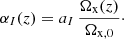
The functional forms of αI(z), I = M, B, K, are not given by the effective description. For simplicity, we use the effective DE parametrisation (Piazza et al. 2014; Bellini & Sawicki 2014) common in the literature,
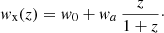
We also allow for deviations from a ΛCDM background by using the Chevallier-Polarski-Linder (CPL; Chevallier & Polarski 2001; Linder 2003) parametrisation for the effective DE equation of state of the Horndeski models:
In summary, the Horndeki model we consider contains five additional free parameters with respect to ΛCDM:

The ΛCDM model is recovered for w0 = −1 and wa = aM = aB = aK = 0.
3. Methodology
The cosmological evolution of the models was computed using the Boltzmann code1 CLASS (Blas et al. 2011), and its modified version2 hi_class (Zumalacarregui et al. 2017; Bellini et al. 2020). The cosmological data – hereafter referred to as the “baseline” – contain the SDSS-II/SNLS3 Joint Light-curve Analysis (JLA) sample of type Ia supernova (SNIa; Betoule et al. 2014), the Baryon Oscillation Spectroscopic Survey (BOSS) baryon acoustic oscillation (BAO) measurements (Beutler et al. 2011; Anderson et al. 2014; Ross et al. 2015), and the low- and high-multipole temperature and polarisation of Planck 2018 cosmic microwave background (CMB) data (Planck Collaboration V 2020). We chose not to include CMB lensing data to avoid inconsistencies related to potential ΛCDM-dependent assumptions made during the lensing reconstruction.
Our aim was to focus on the gain from breaking growth degeneracy, rather than making realistic mocks and forecasts. In order to compare the constraining power of separated measurements of f and σ8 with the combined measurements fσ8, we simulated data for a nominal future galaxy sample that delivered a one percent precision for f, σ8, and fσ8. We assumed a redshift range containing ten measurements at z = 0.1, 0.2, …, 1. The effects of extending the redshift range are studied in Sect. 4.3. We anticipate that a Stage IV experiment conducting a spectroscopic galaxy count survey together with a weak lensing survey, such as Euclid (Amendola et al. 2018), should be able to achieve close to 1% precision on fσ8, f, and σ8, using Planck priors on standard cosmological parameters.
Whenever needed, the growth quantities are computed with CLASS or hi_class. In order to compare the constraints on the same footing and avoid non-linear model dependencies, we computed the growth quantities with the linear power spectrum only. The values of σ8 were obtained via the usual weighted integral of the linear power spectrum and f was computed as the log derivative f = −(1 + z)dlnσ8/dlnz for simplicity.
As fiducial parameters we used the best-fit values obtained from the baseline constraints for the ΛCDM and Horndeski models. Then we created three sets of mocks for both models (for f, σ8, and fσ8), each exactly centred on their fiducial, meaning no random variance added to the data. The ΛCDM model has been shown to lie in a corner of the parameter space of stable Horndeski models (Piazza et al. 2014), which are ghost- and gradient-free models. When performing forecasts using Markov chain Monte Carlo (MCMC) methods, the stability priors can lead to a disfavouring of models lying close to the corner, purely due to volume effects and independently of their actual likelihood. Such considerations may have a significant effect on our results. This is hinted at for example by the highly irregular posteriors in the baseline case in Fig. 3 (grey contours) and the mismatch between their maximum and the best-fit model (dotted lines), characteristic of non-negligible prior effects. We can however expect those effects to be mitigated when additional data is added to the analysis, due to the fact that our Horndeski fiducial model (derived from the baseline best fit and used to produce our mocks) lies noticeably away from the “ΛCDM corner”. Even if our MCMC explorations were impacted by such priors, this should not affect our conclusions since we always make statements regarding relative improvements.
4. Constraints
The sampling of all the considered likelihoods, as well as the computation of best-fit parameters, are performed using the publicly available3 suite of codes ECLAIR (Ilić et al. 2020). It uses as its main sampling algorithm the affine-invariant ensemble method of Foreman-Mackey et al. (2013) and contains a novel and robust maximiser with reliable convergence towards the global maximum of the posterior.
4.1. ΛCDM
Marginalised posterior distributions are shown in Fig. 1. The corresponding means and 68% confidence intervals are given in Table 1, while Table 2 shows the gain in precision relative to the baseline (first two columns) and for the separated growth measurements f + σ8 relative to the standard fσ8 measurements (last column). We define the precision as the inverse width of the 68% marginalised confidence interval rather than using relative errors, since the latter can become misleading when the mean values are close to zero (e.g., in the case of Σmν). In addition, comparing relative errors would also be biased when the mean values shift, as happens for the Horndeski models (see below).
 |
Fig. 1. One-dimensional and two-dimensional marginalised posterior distributions for ΛCDM parameters derived from the baseline only (grey), baseline with mock on fσ8 (blue), and baseline with mocks on f and σ8 (red). The dotted lines indicate the parameter values for the fiducial model (corresponding to the baseline best fit) used when generating mocks. |
Mean and 68% confidence interval for ΛCDM parameters.
Precision ratios for ΛCDM parameters.
Next-generation surveys are forecast to deliver improved constraints from high-precision RSD fσ8 data (see e.g. Amendola et al. 2018; Bacon et al. 2020). The triangle plots and the tables confirm this. Table 2 (first column) shows that the gain in precision ranges from ∼10% for Ωbh2 up to more than ∼50% for Ωch2, H0 and Σmν, when considering the addition of the mock data on fσ8, with 1% relative error combined to current cosmological data sets.
As expected the constraints improve further with the split mock data on f and σ8, each with a 1% relative error. This combination performs from 6% to almost 50% better. In particular, the precision on Ωch2 and H0 is more than doubled relative to the baseline data alone.
The improvement obtained from the split f and σ8 data over fσ8 (as quantified by the third column of Table 2) does not lead to an equal increase in precision on all the parameters that were already well constrained with fσ8 RSD data. As an example, we can compare Σmν and H0. Adding fσ8 data yields almost a 50% gain on Σmν, while the split f + σ8 data further increases the precision by 13%. By contrast, H0 precision first increases by 55% followed by another 46% with the splitting.
The growth probes f, σ8, and fσ8 have different sensitivities to each cosmological parameter, which explains the range of changes in precision. One way to examine those sensitivities is to start with the baseline-only constraints. Figure 2 shows the posterior distributions of f, σ8, and fσ8 at redshift z = 0.1 as derived parameters versus the cosmological parameters4. Each posterior thus illustrates how a change in a given cosmological parameter impacts the values of the derived growth quantities, taking into account (i.e. marginalising over) the remaining cosmological parameters and how their values need to change to keep a decent fit to the data.
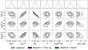 |
Fig. 2. One-dimensional marginalised posterior distributions (top row) for ΛCDM parameters, from baseline only (grey), baseline + mock on f (green), and baseline + mock on σ8 (purple). Rows below show 2D posteriors of cosmological parameters against derived parameters f, σ8, and fσ8 at z = 0.1. |
On the other hand, adding constraints on the growth quantities amounts to convolving their posteriors with a Gaussian distribution (with a width equal to 1% of the central value). This in turn may reduce the width of the posterior on cosmological parameters, depending on the amount of correlation between the two. It is thus expected that cosmological parameters that are highly correlated (i.e. thin tilted ellipses) with a given growth quantity in the baseline case, will show the best improvements after including measurements of that growth quantity.
From Fig. 2 we find that Ωb, Ωc, H0, and ns are better constrained by adding the f mock (green) to the baseline, while τ, As, and Σmν are better constrained by adding the σ8 mock (purple). This may appear counter to the common expectation that σ8 is more sensitive to parameters affecting the power spectrum amplitude, while f is more sensitive to parameters affecting its shape. It is the correlations induced by the baseline constraints that are the decisive factor.
Let us consider an illustrative example from Fig. 2: the 2D posterior of {f(0.1),H0} exhibits a high correlation (thin tilted ellipse), while that of {σ8(0.1),H0} is relatively irregular and close to an uncorrelated case. As a result, the addition of the f mock improves the H0 constraint significantly more relative to the baseline (see the 1D posterior of H0 in the top row of Fig. 2).
These correlations can even lead to improved constraints on parameters that f and σ8 should not depend on. An example is the tight constraint on the reionisation parameter τ produced by the mock on σ8, which originates in the tight constraint on As from σ8, combined with the underlying high correlation between As and τ, as shown in Fig. 1. A tight constraint on τ is obtained even though it does not play a role in the value of σ8.
4.2. Horndeski
The Horndeski parameter space is extended to include modifications in the background (w0, wa) and in the perturbations (αM, αK, αB). Marginalised posterior distributions with the baseline and mock data sets are displayed in Fig. 3, with the corresponding means and 68% confidence intervals in Table 3. We observe that the maximum of the posterior distribution for the extension parameters shifts significantly towards the best-fit model (dotted lines), while the contours assume a much more regular, ellipsoidal shape compared to the baseline case. This is expected in a transition from a regime where priors still play a significant role (as discussed at the end of Sect. 3), to a situation where data dominate the posterior. Interestingly, these results also show that if the true underlying cosmology is indeed close to the Horndeski best-fit fiducial, then growth data with 1% relative precision (over the redshift range considered) could lead to the detection of this deviation from ΛCDM with strong significance (more than 5σ).
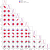 |
Fig. 3. One-dimensional and two-dimensional marginalised posterior distributions for Horndeski parameters derived from the baseline only (grey), baseline with mock on fσ8 (blue), and baseline with mocks on f and σ8 (red). The dotted lines indicate the parameter values for the fiducial model (corresponding to the baseline best fit) used when generating mocks. |
Mean and 68% confidence interval for Horndeski parameters.
Table 4 shows the gain in precision relative to the baseline (first two columns) and for the separated growth measurements f + σ8 relative to the standard fσ8 measurements (last column). As pointed out earlier, the kineticity coupling αK is not constrained by the data and is therefore not included in the figure and tables, but aK is included as a free parameter in the analysis. The accuracy that was gained on the cosmological parameters in ΛCDM is largely lost. Adding the mock on fσ8 only delivers a precision gain of up to ∼20% (see Table 4). This can be attributed to the addition of new, poorly constrained degrees of freedom, which naturally leads to larger errors on all the original parameters via correlations, as both sets may have similar and degenerate effects on the growth of structure. For example, Fig. 3 shows how aM and aB are relatively degenerate with other parameters when using the baseline data only.
Precision ratios for Horndeski parameters.
However, there is significant improvement for the extension parameters: adding future fσ8 data yields a 230% improvement for the running of the effective Planck mass αM and a remarkable ∼50% gain for Σmν. Even though fσ8 is a probe of the perturbations, adding its mock to the baseline achieves a surprising ∼30% and ∼60% gain in precision for w0 and wa respectively.
The additional gain from disentangling f and σ8 measurements is also subject to the effects of opening up the parameter space. The standard parameters see little improvement (< 15%) over the fσ8 case. By contrast, wa, Σmν, and αM precisions jump by a further ∼20%, ∼ 65%, and ∼80% respectively.
The underlying reason why growth data provide such an enhancement in precision for the Horndeski parameters is rooted in the modification of gravitational dynamics (e.g. the Poisson equation) by αI. As discussed in Perenon et al. (2019), these modifications produce two opposing contributions:
⁎ a fifth force, enhancing growth;
⁎ a higher effective Planck mass, suppressing growth.
The effective Planck mass is controlled solely by αM for the models we consider. As a result, growth data strongly constrains aM and also aB. Table 4 shows that the splitting of fσ8 into f and σ8 is very effective to further constrain aM, thereby disentangling the fifth force and effective Planck mass contributions. This feature was seen even with current split data in Perenon et al. (2019).
The modified background parameters w0 and wa also contribute to the growth of structure through Hubble friction. Their effects on growth are therefore degenerate with those of αI. We see in Fig. 4 that w0, wa, aB, and aM display some degeneracies in their 2D marginalised posteriors.
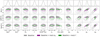 |
Fig. 4. One-dimensional marginalised posterior distributions (top row) for Horndeski parameters, from baseline only (grey), baseline + mock on f (green), and baseline + mock on σ8 (purple). Rows below show 2D posteriors of cosmological parameters against derived parameters f, σ8, and fσ8 computed at z = 0.1. |
Following the arguments for ΛCDM, we can understand the separate improvements from f and σ8 by analysing their posterior distributions versus cosmological parameters, shown in Fig. 4. We note that the stability requirements for the Horndeski models induce highly non-Gaussian posterior distributions, which makes the analysis more subtle. Figure 4 shows that f correlates more strongly with aB and aM than σ8, so that adding f measurements results in a larger increase in precision for these parameters. Since these two parameters control the strength of the fifth force, this could be expected, given that σ8 is an integrated function of f, which tends to wash out the effects of the fifth force. The fifth force is an effect occurring at low redshifts as opposed to the effect of Hubble friction or neutrinos. A chain of correlations – seen in the baseline constraints – shows that σ8 brings a larger gain in precision for w0, wa, and Σmν. This signals therefore a higher sensitivity of σ8 to modifications of gravity spanning longer periods.
It is in fact expected that the effect of neutrinos is partially degenerate with that of modified gravity (see e.g. Wright et al. 2019; Ballardini et al. 2020). Massive neutrinos suppress the growth of structure on small scales, which can either oppose or reinforce modified gravity, depending on whether the fifth force or the Planck mass running is favoured. Horndeski models compatible with current RSD fσ8 constraints produce a suppression of growth at late times (Perenon et al. 2019).
The baseline constraints in Fig. 3 show that the 2D posteriors of Σmν with aB and aM have a fairly irregular shape, while those with w0 and wa are more correlated. More surprisingly, as noted above, Σmν has almost a 50% gain with the addition of the fσ8 mock data, as in the case of ΛCDM. The splitting improves constraints by a further 70% as opposed to 7% in ΛCDM. It is therefore clear that these growth mocks break the neutrino-modified gravity degeneracy by efficiently constraining Σmν and the extension parameters. Figure 4 tells us that this is rooted in the correlation of Σmν with σ8 in the baseline.
On the other hand, we also see that all the intricate degeneracies between the extension parameters and standard model parameters render the baseline constraints for the latter much less correlated than in the case of ΛCDM. This explains why the improvements from the splitting are not as great in the case of Horndeski for the other standard parameters. We note that when the background evolution is fixed to that of ΛCDM, Σmν displays a correlation with αB (Bellomo et al. 2017). Here, the freedom that arises from varying w0 and wa lessens that correlation.
4.3. Extending the redshift range
Having understood better the influence of each mock data set on the constraints, we now assess the effect of extending the redshift coverage of the mocks. More specifically, we examine the respective merits of adding fσ8 or f + σ8 measurements, when extending the maximum redshift of each mock. Table 5 shows that the combined data fσ8 with zmax = 2 (first column) performs no better than f + σ8 data with half the redshift range (zmax = 1, see Tables 1 and 3). We find that extending the redshift range further improves the precision up to 30% with respect to zmax = 1 in the case of the combined mock fσ8 for ΛCDM and Horndeski models, and respectively 20% and 15% in the case of f and σ8 mocks.
Mean and 68% confidence interval for ΛCDM (top) and Horndeski (bottom) parameters with the redshift of the mocks extended to z = 0.1, 0.2, …, 2.0.
5. Conclusion
Upcoming galaxy surveys such as Euclid (Amendola et al. 2018) and Square Kilometre Array (SKA; Bacon et al. 2020) with their unprecedented precision is a call to sharpen our tools for constraining gravity. One cosmological probe well suited for that task is the growth of structure. This toolbox is further complemented by the releases of measurements on f and σ8 (de la Torre et al. 2017; Shi et al. 2018; Jullo et al. 2019; Gil-Marín et al. 2017).
In this paper, we considered the performance that a future nominal galaxy sample can deliver with a ∼1% relative error on f and σ8 separately and on the combination fσ8. We compared the constraints from the separated data with those from the combination data. We assumed ten measurements per growth quantity equally spread over the redshift range z = 0.1, 0.2, …, 1.0. For the case of ΛCDM, the improvements in precision range over ∼5–50%. For modified gravity described by Horndeski models, the improvements on these standard model parameters reduce to ∼0–15%.
However, the splitting of f and σ8 stands out as very effective in breaking the neutrino – modified gravity degeneracy, with the sum of neutrino masses enjoying an improvement of 65% over the case with only fσ8 data. We also find a significant increase in the precision on the background and perturbation Horndeski parameters, with an additional gain of ∼20% for the varying effective DE equation of state parameter wa and ∼80% for the evolution of the effective Planck mass aM. Extending the redshift of the mocks up to zmax = 2 shows that the constraints provided by the combined fσ8 data are already matched by the split data f and σ8 with zmax = 1.
Our results highlight that growth data, whether split or combined and with 1% relative error could lead to the detection of deviations from ΛCDM with strong significance (more than 5σ), should the underlying cosmology be close to the current Horndeski best-fit fiducial. The splitting of growth data on fσ8 into data on f and σ8 with galaxy-galaxy lensing (de la Torre et al. 2017; Shi et al. 2018; Jullo et al. 2019) or by combinations with the bispectrum (Gil-Marín et al. 2017) emerges clearly from this work as both a powerful complementary probe for the standard model and a stringent probe to detect departures from it. The latter could prove crucial in the era of future surveys, given the current tensions within the standard model and the emergence of alternative models of gravity favoured by Bayesian evidence (Peirone et al. 2019; Solà Peracaula et al. 2019).
Acknowledgments
We are grateful to Julien Bel for helpful exchanges and feedback on the draft. We thank Matteo Martinelli for useful discussions. The authors acknowledge the Sciama High Performance Compute Cluster, which is supported by the ICG at the University of Portsmouth, and the CHPC the Centre for High Performance Computing (CHPC), South Africa, for providing computational resources for this research project. LP and RM are supported by the South African Radio Astronomy Observatory (SARAO) and the National Research Foundation (Grant No. 75415). RM is also supported by the UK STFC Consolidated Grant ST/N000668/1. SI was supported by the European Structural and Investment Fund and the Czech Ministry of Education, Youth and Sports (Project CoGraDS – CZ.02.1.01/0.0/0.0/15_003/0000437). AdlCD acknowledges financial support from NRF Grants No.120390, Reference: BSFP190416431035 and No.120396, Reference: CSRP190405427545, Project No. FPA2014-53375-C2-1-P from the Spanish Ministry of Economy and Science, Project No. FIS2016-78859-P from the European Regional Development Fund and Spanish Research Agency (AEI), and support from Projects Nos. CA15117 and CA16104 from COST Actions EU Framework Programme Horizon 2020.
References
- Abazajian, K. N., Adshead, P., Ahmed, Z., et al. 2016, ArXiv e-prints [arXiv:1610.02743] [Google Scholar]
- Abbott, B., Abbott, R., Abbott, T. D., et al. (LIGO Scientific Collaboration and Virgo Collaboration) 2017a, Phys. Rev. Lett., 119, 161101 [NASA ADS] [CrossRef] [PubMed] [Google Scholar]
- Abbott, B., Abbott, R., Abbott, T. D., et al. 2017b, ApJ, 848, L13 [NASA ADS] [CrossRef] [Google Scholar]
- Alonso, D., Bellini, E., Ferreira, P. G., & Zumalacarregui, M. 2017, Phys. Rev. D, 95, 063502 [NASA ADS] [CrossRef] [Google Scholar]
- Amendola, L., Appleby, S., Avgoustidis, A., et al. 2018, Liv. Rev. Rel., 21, 2 [Google Scholar]
- Anderson, L., Aubourg, É., Bailey, S., et al. 2014, MNRAS, 441, 24 [NASA ADS] [CrossRef] [Google Scholar]
- Bacon, D. J., Battye, R. A., Bull, P., et al. 2020, PASA, 37, e007 [CrossRef] [Google Scholar]
- Ballardini, M., Sapone, D., Umiltà, C., Finelli, F., & Paoletti, D. 2019, JCAP, 05, 049 [CrossRef] [Google Scholar]
- Ballardini, M., Braglia, M., Finelli, F., et al. 2020, JCAP, 2020, 008 [Google Scholar]
- Bellini, E., & Sawicki, I. 2014, JCAP, 1407, 050 [NASA ADS] [CrossRef] [Google Scholar]
- Bellini, E., Cuesta, A. J., Jimenez, R., & Verde, L. 2016, JCAP, 1602, 053; erratum: JCAP1606, no.06, E01(2016) [CrossRef] [Google Scholar]
- Bellini, E., Sawicki, I., & Zumalacarregui, M. 2020, J. Cosmol. Astropart. Phys., 2, 008 [CrossRef] [Google Scholar]
- Bellomo, N., Bellini, E., Hu, B., et al. 2017, JCAP, 1702, 043 [CrossRef] [Google Scholar]
- Betoule, M., Kessler, R., Guy, J., et al. 2014, A&A, 568, A22 [NASA ADS] [CrossRef] [EDP Sciences] [Google Scholar]
- Beutler, F., Blake, C., Colless, M., et al. 2011, MNRAS, 416, 3017 [NASA ADS] [CrossRef] [Google Scholar]
- Blas, D., Lesgourgues, J., & Tram, T. 2011, JCAP, 1107, 034 [NASA ADS] [CrossRef] [Google Scholar]
- Bloomfield, J. K., Flanagan, E. A., Park, M., & Watson, S. 2013, JCAP, 1308, 010 [NASA ADS] [CrossRef] [Google Scholar]
- Chevallier, M., & Polarski, D. 2001, Int. J. Mod. Phys. D, 10, 213 [NASA ADS] [CrossRef] [Google Scholar]
- de la Torre, S., Guzzo, L., Peacock, J. A., et al. 2017, A&A, 608, A44 [NASA ADS] [CrossRef] [EDP Sciences] [Google Scholar]
- Foreman-Mackey, D., Hogg, D. W., Lang, D., & Goodman, J. 2013, PASP, 125, 306 [CrossRef] [Google Scholar]
- Frusciante, N., & Perenon, L. 2020, Phys. Rept., 857, 1 [CrossRef] [Google Scholar]
- Frusciante, N., Peirone, S., Casas, S., & Lima, N. A. 2019, Phys. Rev. D, 99, 063538 [CrossRef] [Google Scholar]
- Gil-Marín, H., Percival, W. J., Verde, L., et al. 2017, MNRAS, 465, 1757 [NASA ADS] [CrossRef] [Google Scholar]
- Gleyzes, J., Langlois, D., Mancarella, M., & Vernizzi, F. 2016, JCAP, 02, 056 [CrossRef] [Google Scholar]
- Gubitosi, G., Piazza, F., & Vernizzi, F. 2013, JCAP, 1302, 032 [NASA ADS] [CrossRef] [Google Scholar]
- Horndeski, G. W. 1974, Int. J. Theor. Phys., 10, 363 [CrossRef] [MathSciNet] [Google Scholar]
- Ilić, S., Kopp, M., Skordis, C., & Thomas, D. B. 2020, A&A, submitted [arXiv:2004.09572] [Google Scholar]
- Jullo, E., de la Torre, S., Cousinou, M.-C., et al. 2019, A&A, 627, A137 [CrossRef] [EDP Sciences] [Google Scholar]
- Kreisch, C. D., & Komatsu, E. 2018, JCAP, 1812, 030 [CrossRef] [Google Scholar]
- Leung, J. S.-Y., & Huang, Z. 2017, Int. J. Mod. Phys. D, 26, 1750070 [CrossRef] [Google Scholar]
- Linder, E. V. 2003, Phys. Rev. Lett., 90, 091301 [NASA ADS] [CrossRef] [PubMed] [Google Scholar]
- Peirone, S., Benevento, G., Frusciante, N., & Tsujikawa, S. 2019, Phys. Rev. D, 100, 063540 [CrossRef] [Google Scholar]
- Perenon, L., Bel, J., Maartens, R., & de la Cruz-Dombriz, A. 2019, JCAP, 1906, 020 [CrossRef] [Google Scholar]
- Piazza, F., Steigerwald, H., & Marinoni, C. 2014, JCAP, 1405, 043 [Google Scholar]
- Planck Collaboration V. 2020, A&A, 641, A5 [CrossRef] [EDP Sciences] [Google Scholar]
- Reischke, R., Spurio Mancini, A., Schafer, B. M., & Merkel, P. M. 2019, MNRAS, 482, 3274 [Google Scholar]
- Ross, A. J., Samushia, L., Howlett, C., et al. 2015, MNRAS, 449, 835 [NASA ADS] [CrossRef] [Google Scholar]
- Shi, F., Yang, X., Wang, H., et al. 2018, ApJ, 861, 137 [NASA ADS] [CrossRef] [Google Scholar]
- Solà Peracaula, J., Gomez-Valent, A., de Cruz Pérez, J., & Moreno-Pulido, C. 2019, ApJ, 886, L6 [CrossRef] [Google Scholar]
- Spurio Mancini, A., Reischke, R., Pettorino, V., Schafer, V., & Zumalacárregui, M. 2018, MNRAS, 480, 3725 [CrossRef] [Google Scholar]
- Wright, B. S., Koyama, K., Winther, H. A., & Zhao, G.-B. 2019, JCAP, 06, 040 [CrossRef] [Google Scholar]
- Zumalacarregui, M., Bellini, E., Sawicki, I., Lesgourgues, J., & Ferreira, P. G. 2017, JCAP, 1708, 019 [CrossRef] [Google Scholar]
All Tables
Mean and 68% confidence interval for ΛCDM (top) and Horndeski (bottom) parameters with the redshift of the mocks extended to z = 0.1, 0.2, …, 2.0.
All Figures
|
Fig. 1. One-dimensional and two-dimensional marginalised posterior distributions for ΛCDM parameters derived from the baseline only (grey), baseline with mock on fσ8 (blue), and baseline with mocks on f and σ8 (red). The dotted lines indicate the parameter values for the fiducial model (corresponding to the baseline best fit) used when generating mocks. |
| In the text | |
|
Fig. 2. One-dimensional marginalised posterior distributions (top row) for ΛCDM parameters, from baseline only (grey), baseline + mock on f (green), and baseline + mock on σ8 (purple). Rows below show 2D posteriors of cosmological parameters against derived parameters f, σ8, and fσ8 at z = 0.1. |
| In the text | |
|
Fig. 3. One-dimensional and two-dimensional marginalised posterior distributions for Horndeski parameters derived from the baseline only (grey), baseline with mock on fσ8 (blue), and baseline with mocks on f and σ8 (red). The dotted lines indicate the parameter values for the fiducial model (corresponding to the baseline best fit) used when generating mocks. |
| In the text | |
|
Fig. 4. One-dimensional marginalised posterior distributions (top row) for Horndeski parameters, from baseline only (grey), baseline + mock on f (green), and baseline + mock on σ8 (purple). Rows below show 2D posteriors of cosmological parameters against derived parameters f, σ8, and fσ8 computed at z = 0.1. |
| In the text | |
Current usage metrics show cumulative count of Article Views (full-text article views including HTML views, PDF and ePub downloads, according to the available data) and Abstracts Views on Vision4Press platform.
Data correspond to usage on the plateform after 2015. The current usage metrics is available 48-96 hours after online publication and is updated daily on week days.
Initial download of the metrics may take a while.