| Issue |
A&A
Volume 642, October 2020
|
|
|---|---|---|
| Article Number | A114 | |
| Number of page(s) | 10 | |
| Section | Galactic structure, stellar clusters and populations | |
| DOI | https://doi.org/10.1051/0004-6361/202038625 | |
| Published online | 12 October 2020 | |
Strömgren metallicities for intermediate-age and old star clusters
1
Instituto Interdisciplinario de Ciencias Básicas (ICB), CONICET-UNCUYO, Padre J. Contreras 1300, M5502JMA Mendoza, Argentina
e-mail: This email address is being protected from spambots. You need JavaScript enabled to view it.
2
Consejo Nacional de Investigaciones Científicas y Técnicas (CONICET), Godoy Cruz 2290, C1425FQB Buenos Aires, Argentina
Received:
9
June
2020
Accepted:
12
August
2020
We report results that show that the straightforward star cluster metallicities obtained from Strömgren vby photometry are age-dependent and need to be corrected for further use. This outcome arises from the comparison of [Fe/H] values derived from Strömgren photometry with those metallicities published in the literature for 26 Large and Small Magellanic Cloud star clusters, whose ages range from ∼1 Gyr up to the oldest-known globular cluster ages in these galaxies. While deriving mean star cluster metallicities, we carried out a thorough selection of red giant branch candidates to comply with the Strömgren metallicity calibration validity regime. We paid attention to the effect of contamination by field stars, particularly those that lie inside the star clusters’ radii, that are distributed along the star cluster red giant branches and that have [Fe/H] values covering a similar range as that for the selected stars. We find that the measured Strömgren metallicities are systematically more metal-poor than the published ones and that a quadratically age-varying function reproduces the relative metallicity values with an overall uncertainty of ∼0.05 dex. We finally performed a similar comparison relying on a fully independent approach, which consisted in using theoretical red giant branches of old globular clusters spanning [Fe/H] values from −2.0 up to 0.0 dex as standards. We then superimposed onto them the red giant branches of star clusters with ages in the range 1.0−12.5 Gyr and estimated their associated metallicities by interpolation. The derived theoretical relative metallicities follow a similar trend as a function of the star clusters’ ages as what has been found from observations of star clusters.
Key words: methods: observational / techniques: photometric / globular clusters: general / open clusters and associations: general / stars: abundances
© ESO 2020
1. Introduction
Star clusters’ metallicities have long been used as key parameters for unveiling the chemical evolution of galaxies. Their metal abundances tell us about, among other things, the efficiency of the gas mixing within a galaxy, the metal enrichment throughout the galaxy’s lifetime, and the infall of gas from galaxy interactions. Alongside ages and positions (age-metallicity relationships and metallicity gradients), star clusters’ metallicities have helped us in understanding whether galaxies formed through outside-in or inside-out formation scenarios, detecting the existence of bursting formation episodes that produced a sudden chemical enrichment, and estimating the effectiveness of scattering star clusters, among others.
In this context, the red giant branch of old star clusters has been employed to estimate metallicities from a variety of photometric systems, namely: Johnson BV (Hartwick 1968), Johnson-Cousins VI (Da Costa & Armandroff 1990), Washington CT1 (Geisler & Sarajedini 1999), near-infrared J, Ks bands (Frogel et al. 1983), etc. This is because the colors of the red giant branch stars show sensitivity to changes in metallicities. The result is that the red giant branches appear shifted toward bluer regions in the color-magnitude diagram (CMD) as the star clusters are more metal-poor. In practice, a fixed magnitude level was adopted and the color differences at that magnitude level were obtained and transformed into [Fe/H] values. Nevertheless, having a long and well-populated red giant branch is advantageous since it can be superimposed onto the standard iso-abundance red giant branches and thus allows us to obtain a metallicity estimate by interpolation.
These iso-abundance red giant branches have usually been drawn from CMDs of old globular clusters; as such, when using them for estimating metallicities of younger star clusters, the derived [Fe/H] values result much more metal-poor because of the age-metallicity degeneracy. This phenomenon has been studied from numerical simulations for the Johnson VI photometric system by Ordoñez & Sarajedini (2015), who show that the metallicity derived from the star cluster’s red giant branch stars can be in error by up to ∼0.5 dex if the star cluster is younger than ∼6 Gyr. Geisler et al. (2003) also derived an age-dependent metallicity correction for the Washington CT1 photometric system, which shows that [Fe/H] values of star clusters of ∼1 Gyr need to be corrected by ∼0.7 dex in order to compute reliable metallicities.
The Strömgren vby medium-bandwidth filters (Crawford & Mandwewala 1976) have proved to be able to derive straightforwardly accurate metallicity values ([Fe/H]) for many stars in a star cluster field, provided the photometric data are precise (see, e.g., Frank et al. 2015; Massari et al. 2016; Gruyters et al. 2017). This is because the index m1 = (v − b)−(b − y) has resulted to be a metallicity-sensitive one, as judged by the available calibrations of it as a photometric proxy of iron abundances. In particular, the semiempirical calibration obtained by Calamida et al. (2007) has turned out to be the most robust for estimating metallicities of red giants (Adén et al. 2009; Calamida et al. 2009; Árnadóttir et al. 2010). It was derived using high-dispersion spectroscopic data of red giants of Milky Way globular clusters and alpha-enhanced isochrones transformed to the observational plane by using semiempirical color-temperature relations.
In this work, we present Strömgren vby photometry of intermediate-age Large and Small Magellanic Clouds (LMC; SMC) star clusters with the aim to investigate to what extent Strömgren metallicities are affected by the age-metallicity degeneracy. If such an age-metallicity dependency exists, it should arise from the comparison of the metallicities measured here from the Strömgren indices with the accurate values available in the literature. The paper is organized as follows: Sect. 2 introduces the obtained Strömgren vby images and describes how they were processed to obtain the standardized photometric data sets. Sections 3 and 4 deal with the metallicity estimates and the aforementioned age-metallicity correction. Finally, Sect. 5 summarizes the main results of this work. We note that a metallicity calibration based on young stellar evolutionary models would be of great value. Such a calibration should consider the different evolutionary statuses of young stars (∼1 Gyr) compared to old stars (> 10 Gyr) in different Strömgren color planes.
2. Strömgren photometric data
We made use of Strömgren vby images collected during the observing program SO2008B-0917 (PI: Pietrzyński) conducted with the SOAR Optical Imager (SOI) attached to the 4.1m Southern Astrophysical Research (SOAR) telescope (FOV = 5.25′ × 5.25′, scale = 0.154″ px−1 in binned mode). The observing program was executed during two different epochs (December 17−19, 2008, and January 16−18, 2009) under excellent image quality conditions (typical FWHM ∼ 0.6″). We downloaded the observational material from the National Optical Astronomy Observatory (NOAO) Science Data Management (SDM) archives1. Table 1 lists the log of observations for the studied LMC and SMC star clusters.
Observing log and properties of the LMC-SMC star cluster sample.
We processed the images following the SOI’s reduction prescriptions2 and thus used nightly zero and flat-field images. As for the photometry standardization, we employed observations of the following Strömgren standard stars: HD 64, HD 3417, HD 12756, HD 22610, HD 57568, HD 58489, HD 66020, TYC 7547-711-1, TYC 7548-698-1, TYC 7583-1011-1, TYC 7583-1622-1, TYC 7626-763-1, TYC 8033-906-1, TYC 8067-207-1, TYC 8104-856-1, and TYC 8104-969-1 (Hauck & Mermilliod 1998; Paunzen 2015). They were observed in all the vby filters at airmasses spanning the range ∼1.02−2.20. Standard stars were observed at a fixed airmass twice to allow them to be placed in the two different CCDs arrayed by SOI, and thus to monitor their individual responses. Piatti & Bailin (2019) show that the transformation coefficients obtained from magnitudes of standard stars placed in each CCD are indistinguishable, so we enlarged the sample of standard star magnitude measurements by considering all of them irrespective of their positions in the SOI. To convert instrumental magnitudes into standard ones, we first gathered all the information of the standard stars and then fit the following expressions:


where vi, bi, and yi are the ith fit coefficients and X represents the effective airmass. The resulting mean transformation coefficients are listed in Table 2 of Piatti et al. (2019), who used images from the same observing program to estimate metallicities of young star clusters in the LMC and SMC from their supergiant populations.
We relied on the routine packages DAOPHOT, ALLSTAR, DAOMATCH, and DAOMASTER (stand-alone version, Stetson et al. 1990) to obtain point-spread-function (PSF) photometric data sets of the star clusters’ fields and their associated uncertainties. In order to build the PSF of an image, we first interactively selected nearly 100 well-isolated, relatively bright, non-saturated stars, distributed over the whole image area. A subsample of nearly 40 of the best PSF stars was used to build a preliminary PSF, which was applied to the image with the aim of cleaning the entire PSF star sample from fainter neighbors. With the cleaned PSF stars, we constructed the final quadratically spatially varying PSF for that image and computed aperture corrections that resulted in the range −0.04 to −0.07 mag. The PSF was applied to the entire list of identified stellar sources in the image. The resulting subtracted image was employed to identify new ones, which were simultaneously fit by the PSF with those in the previous list. We took advantage of this procedure of enlarging the photometrically measured star sample by iterating it three times. Their standard magnitudes were obtained by inverting Eqs. (1)−(3) and entering the computed instrumental magnitudes. The procedure described above was repeated for each of the images listed in Table 1. In the subsequent analysis, we only kept those stellar sources with χ < 2, and |SHARPNESS| < 0.5. Both, χ and SHARPNESS are image quality diagnostic parameters used by DAOPHOT. We adopted the frequently used values of χ and SHARPNESS to exclude bad pixels, cosmic rays, galaxies, and unrecognized double stars.
In order to quantify the uncertainties associated with the obtained photometry, we followed the recipe applied in previous studies of other subsets of star clusters observed during the same observing program (see Piatti & Koch 2018; Piatti 2018). The method consists in adding synthetic stars with magnitudes and positions distributed similarly to those of the measured stars to an image, and carrying out the photometry for the new image as described above. The synthetic stars represent nearly 5% of the measured stars, so the original image stellar density is not significantly altered. The resulting magnitudes for the synthetic stars were then compared with those used to create such stars. The difference between them typically turned out to equal zero and in all cases was smaller than 0.003 mag. We then decided to use the root-mean-square errors obtained from the comparison of input and output synthetic star magnitudes as photometric errors.
3. Metallicity estimates
The metallicity calibration obtained by Calamida et al. (2007) involves the m10 and (v − y)0 indices of red giant branch stars, corrected by reddening, according to the following expression:
![$$ \begin{aligned} {m_{1}}_0 = \alpha + \beta \mathrm{[Fe/H]} + \gamma ({ v}-{ y})_0 + \delta \mathrm{[Fe/H]}({ v}-{ y})_0 , \end{aligned} $$](/articles/aa/full_html/2020/10/aa38625-20/aa38625-20-eq4.gif)
where α = −0.309, β = −0.090 ± 0.002, γ = 0.521 ± 0.001, and δ = 0.159 ± 0.001. While de-reddening color indices is a somewhat straightforward task, the selection of red giant branch stars requires several steps. We retrieved the E(B − V) values obtained by Schlafly & Finkbeiner (2011) from the NASA/IPAC Infrared Science Archive3 (see Table 1) using the star clusters’ coordinates and computed the intrinsic colors:

and

where the reddening ratios E(X)/E(B − V), for X = v − y and m1, are those given by Crawford & Mandwewala (1976). The (v − y)0 and m10 values were then entered into Eq. (4) to compute individual stellar metallicities. Their errors were estimated from a full analytical propagation of errors, including those on the calibration coefficients, as follows:
![$$ \begin{aligned} \sigma (\mathrm{[Fe/H]})^2 =&\left(\frac{\partial \mathrm{[Fe/H]}}{\partial \alpha } \sigma (\alpha )\right)^2 + \left(\frac{\partial \mathrm{[Fe/H]}}{\partial \beta } \sigma (\beta )\right)^2\\&+ \left(\frac{\partial \mathrm{[Fe/H]}}{\partial \gamma }\sigma (\gamma )\right)^2 + \left(\frac{\partial \mathrm{[Fe/H]}}{\partial \delta }\sigma (\delta )\right)^2\\&+ \left(\frac{\partial \mathrm{[Fe/H]}}{\partial {m_{\rm 1}}_0}\sigma ({m_{\rm 1}}_0)\right)^2 + \left(\frac{\partial \mathrm{[Fe/H]}}{\partial ({ v}-{ y})_0}\sigma (({ v}-{ y})_0)\right)^2,\end{aligned} $$](/articles/aa/full_html/2020/10/aa38625-20/aa38625-20-eq7.gif)
![$$ \begin{aligned} \sigma (\mathrm{[Fe/H]})^2 =&\left(\frac{0.002\mathrm{[Fe/H]}}{c}\right)^2 + \left(\frac{0.001({ v}-{ y})_0}{c}\right)^2\\&+ \left(\frac{0.001\mathrm{[Fe/H]}({ v}-{ y})_0}{c}\right)^2 + \left(\frac{\sigma ({m_{\rm 1}}_0)}{c}\right)^2\\&+ \left(\frac{(-0.521c - 0.159({m_{\rm 1}}_0 +0.309 -0.521({ v}-{ y})_0)\sigma (({ v}-{ y})_0)}{c^2}\right)^2, \end{aligned} $$](/articles/aa/full_html/2020/10/aa38625-20/aa38625-20-eq8.gif)
where c = −0.090 + 0.159(v − y)0, and σ(m10) and σ((v − y)0) are the photometric errors in m10 and (v − y)0, respectively. The mean star clusters’ metallicities were calculated using the individual [Fe/H] values of the selected stars weighed by their respective uncertainties (see the last column of Table 1). In Appendix A, we provide a comparison of the [Fe/H] values derived for the selected stars (filled red circles in Figs. 1–8) from the semiempirical calibration with those based on the empirical and theoretical calibrations.
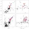 |
Fig. 1. V vs. b − y CMD for measured stars distributed inside the star cluster’s radius (left panels) and their metallicity ([Fe/H]) distribution as a function of the V magnitude (right panels). The large filled red and blue circles represent stars used to compute the star cluster’s mean [Fe/H] value and those from a reference star field with [Fe/H] values similar to those of the star cluster’s stars, respectively (see text for details). Top and bottom panels: refer to NGC 1651 and 1795, respectively. |
The star clusters’ red giant branch stars were selected according to the following three criteria. First, the stars are located inside the clusters’ radii (Hill & Zaritsky 2006; Bica et al. 2008; Werchan & Zaritsky 2011). This is a basic starting point because contamination from field stars is also present inside those areas. Furthermore, intermediate-age and old LMC-SMC star clusters are frequently projected toward star fields with similar ages and metallicities (Geisler et al. 2003; Piatti 2011b), which means that they also populate the star cluster CMD regions. Second, they are distributed along the red giant branch and above the star cluster red clump-horizontal branch in the V versus b − y CMD; b − y is mainly a temperature effective indicator with less metallicity sensitivity (Crawford & Mandwewala 1976). We initially imposed the simple restrictions V < 18.7 mag and b − y > 0.4 mag (see Figs. 1–8, left panels). These magnitude and color cuts still allow several field stars to appear not only along the star clusters’ red giant branches, but also far away of them. Stars outside the red giant branches were later easily discarded when applying the metallicity cut. Third, the star clusters’ red giant branch stars span a readily visible range of [Fe/H] values in the V versus [Fe/H] plane. Figures 1–8 (right panels) highlight them with large filled red circles; all the stars distributed within the star clusters’ radii that have a metallicity estimate from Eq. (4) are also shown with black dots, irrespective of whether or not they are red giant branch stars (see also Appendix C).
While identifying the star clusters’ red giant branch candidates, we considered the [Fe/H] errors (σ[Fe/H]). Figure 9 shows σ[Fe/H] as a function of V for all the selected stars. As can be seen, the fainter the star, the larger the σ[Fe/H]. For this reason, we gave more weight to the brightest stars with more accurate photometry and hence with the smallest [Fe/H] uncertainties. Likewise, as the V magnitude increases, both σ[Fe/H] and the dispersion of the individual [Fe/H] values increase because of the poorer photometry quality, so that the observed [Fe/H] range of the brightest selected stars more properly reveals the star cluster metallicity range. This metallicity range should be the same at any magnitude level. We also bore in mind that stars distributed along or adjacent to the star clusters’ red giant branches could be field stars with ages differing from those of the star clusters (and hence have different metallicities). These stars spuriously produce a wider spread of [Fe/H] values for relatively bright V magnitudes. The combined population of field and star cluster red clump stars also produces wide ranges of [Fe/H] values. Here we did not use those stars but kept them in Figs. 1–8 for illustrative purposes.
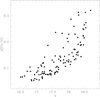 |
Fig. 9. Individual metallicity errors as a function of the V magnitude of stars selected in a star cluster, represented by large filled red circles in Figs. 1–8. |
4. Analysis
We evaluated the degree of contamination by field stars in the resulting mean star cluster metallicities. We are interested in those stars that lie along the star clusters’ red giant branches and have metallicities close to the star clusters’ values. These stars play a role when computing the mean star cluster metallicities because we cannot distinguish them from cluster stars without the availability of proper motions or radial velocities. We used different equal star cluster areas located reasonably far from the star clusters and counted the number of stars (Nfield, represented with filled blue circles in Figs. 1–8) distributed inside them that satisfy the criteria required for the selected red giant branch stars (Ncls). We then computed the ratio Nfield/Ncls and built Fig. 10, which depicts its variation as a function of Ncls. As can be seen, half of the star cluster sample is affected by a mean null field star contamination. SL 549 amounts to 50% of the contribution from field stars in the derived mean metallicity. Nevertheless, Fig. 5 (right panels) shows that this is because of the small number of stars used. These field stars could increase the standard deviation up to ∼0.03 dex, but the mean metallicity value would not change. A similar interpretation could be applied to the remaining stars clusters, where the smaller the Nfield/Ncls ratio, the smaller the increase in the respective standard deviation.
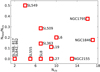 |
Fig. 10. Ratio of the number of stars in the field and the ratio of the number of stars in the star clusters vs. the number of selected stars in each star cluster. |
We searched the literature for ages and metallicities of the studied star cluster sample. Appendix B deals with the individual values available in the literature, while the adopted values are listed in Table 1. From that piece of information (see Table B.1), we computed the difference between the individual reference star clusters’ metallicities and the values derived in this work, distinguishing those coming from high-resolution spectroscopy, low-resolution spectroscopy, or photometry. Figure 11 shows the relationship between the resulting metallicity differences (present – reference) and the star clusters’ ages. We only used reference [Fe/H] values lower than −0.5 dex and included their associated errors so they complied with the metallicity range of Eq. (4). We used all clusters listed in Table 1 except NGC 1795 and SL 817. The point sizes are proportional to Ncls, while their error bars come from adding in quadrature the uncertainties of the reference (Table B.1) and the present mean [Fe/H] values included in Table 1. The points are colored according to the Nfield/Ncls ratios. Figure 11 reveals that the Strömgren metallicities derived from Eq. (4) are age-dependent, and, therefore, they need to be corrected for further use. A general trend is readily visible, which points to the need for discarding some individual discrepant [Fe/H] values. In order to have a second reference source, we used the [Fe/H] values derived from Strömgren theoretical isochrones (Bressan et al. 2012, Y = 0.2485 + 1.78Z, Z⊙ = 0.0152) to superimpose them onto Fig. 11 (open magenta diamonds). We first built V versus (v − y)0 and V versus m10 CMDs for [Fe/H] = −2.0, −1.5, −1.0, −0.5, and 0.0 dex and log(age/yr) = 10.10, which we called standard giant branches. We only drew the red giant branch track sections of these five theoretical isochrones. Then, we superimposed onto these standard giant branches the theoretical red giant branches of isochrones with log(age/yr) = 9.0 and the five [Fe/H] values as for log(age/yr) = 10.10 (see Fig. 12). Because of the age-metallicity degeneracy, the log(age/yr) = 9.0 red giant branches appear shifted toward bluer colors with respect to the corresponding standard red giant branches according to their metallicities. We estimated the [Fe/H] values of the log(age/yr) = 9.0 red giant branches by interpolating in the five standard giant branches and computed the difference between the obtained interpolated [Fe/H] values and those given by the respective isochrones ([Fe/H] = −2.0, −1.5, −1.0, −0.5, and 0.0 dex). We repeated this procedure for log(age/yr) = 9.4 and 9.8. By using these theoretical points and the general trend observed in Fig. 11, we adopted weighted mean [Fe/H] values for each cluster (see Table 1). Figure 13 depicts the resulting distribution using the adopted mean metallicities.
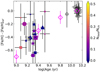 |
Fig. 11. Metallicity difference as a function of the star cluster’s age. Filled circles, squares, and triangles correspond to high-resolution spectroscopy, low-resolution spectroscopy, and photometry reference values, respectively. Open magenta diamonds represent metallicity differences derived from theoretical isochrones (see text for details). |
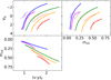 |
Fig. 12. Theoretical red giant branches for log(age/yr) = 9.0 (dotted lines) and 10.10 (solid lines); [Fe/H] = −2.0, −1.5, −1.0, −0.5, and 0.0 dex shown with blue, magenta, green, orange, and red, respectively. |
With the aim of providing an expression for the metallicity correction that covers a wide age range, we added ten LMC old globular clusters studied by Piatti & Koch (2018) from Strömgren photometry. We took from that study the star clusters’ ages as well as both reference and Strömgren metallicities, with their respective uncertainties. They are represented in Figs. 11 and 13 with open circles. When performing a least square fit to all the data points, we obtained the following expression:
![$$ \begin{aligned} \Delta \mathrm{[Fe/H]\,(dex)} =&-41.80({\pm }43.48) + 8.11({\pm }9.00)\\&\times \log (\mathrm{age/yr}) - 0.39({\pm }0.46)\times \log (\mathrm{age/yr})^2, \end{aligned} $$](/articles/aa/full_html/2020/10/aa38625-20/aa38625-20-eq9.gif)
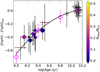 |
Fig. 13. Same as Fig. 11 for adopted weighted mean [Fe/H] values. The solid line represents the least squared fit obtained (see text for details). |
with a standard deviation, a correlation factor, and an F-test coefficient of 0.05, 0.98, and 0.97, respectively. Strömgren metallicities calculated from Eq. (4) should be corrected by an amount equal to −Δ[Fe/H].
5. Summary
Based on our previous knowledge that metallicities derived from standard giant branches in several photometric systems are affected by the age-metallicity degeneracy for star clusters younger than the old globular clusters, and bearing in mind the fundamental role that metallicities play in our understanding of the formation and chemical evolution processes at different universe scales, we decided to investigate metallicities for the Strömgren vby bandpasses. Until now, it has been straightforward to compute [Fe/H] values from the Strömgren reddening free (v − y)0 and m10 indices, the latter being a metallicity-sensitive index. In general, they have been used for the study of globular cluster metallicity distributions (e.g., Calamida et al. 2014; Frank et al. 2015) to unveil multiple stellar populations (e.g., Carretta et al. 2011; Massari et al. 2016) rather than estimate the metal content of intermediate-age star clusters.
In order to probe whether such an age dependency also affects the Strömgren metallicities, we made use of unexploited publicly available Strömgren vby images of intermediate-age and old LMC-SMC star clusters, which had previously been targeted for independent metallicity analysis. Once we properly processed the observational material and standardized the resulting instrumental photometry, we computed individual stellar [Fe/H] values using the semiempirical Calamida et al. (2007) calibration. We performed a sound selection of star cluster red giant branch candidates in order to comply with the metallicity calibration validity. In doing so, we constrained the cluster stars to be distributed inside the star clusters’ radii, located along the star cluster red giant branch, and with [Fe/H] values within the readily visible star cluster metallicity range. We further assessed the effect of the contamination of field stars that are indistinguishable without proper motions or radial velocity measurements from the selected stars used to compute those mean values on the derived mean star cluster metallicities.
The resulting mean [Fe/H] values and the estimated uncertainties were then compared with those metallicities taken from the literature. We find that the measured Strömgren metallicities need to be corrected by an amount that depends on the star cluster age: the younger the star cluster, the larger the metallicity correction. Since the measured [Fe/H] values result more metal-poor than the reference [Fe/H] ones, a positive correction should be added to the former. From 26 relative metallicity points spanning from ∼1 Gyr up to the globular cluster ages, we fit a quadratically age-varying curve that provides metallicity corrections with an overall uncertainty of ∼0.05 dex. We finally repeated a similar comparison from a fully independent approach, which consisted in using theoretical red giant branches to trace the standard red giant branches and those of star clusters with ages in the aforementioned age range. Our findings show a very good agreement between the measured relative metallicities and those derived from theoretical isochrones.
Acknowledgments
I thank the referee for the thorough reading of the manuscript and timely suggestions to improve it.
References
- Adén, D., Feltzing, S., Koch, A., et al. 2009, A&A, 506, 1147 [NASA ADS] [CrossRef] [EDP Sciences] [Google Scholar]
- Árnadóttir, A. S., Feltzing, S., & Lundström, I. 2010, A&A, 521, A40 [NASA ADS] [CrossRef] [EDP Sciences] [Google Scholar]
- Bertelli, G., Nasi, E., Girardi, L., et al. 2003, AJ, 125, 770 [NASA ADS] [CrossRef] [Google Scholar]
- Bica, E., Geisler, D., Dottori, H., et al. 1998, AJ, 116, 723 [NASA ADS] [CrossRef] [Google Scholar]
- Bica, E., Bonatto, C., Dutra, C. M., & Santos, J. F. C. 2008, MNRAS, 389, 678 [NASA ADS] [CrossRef] [Google Scholar]
- Bressan, A., Marigo, P., Girardi, L., et al. 2012, MNRAS, 427, 127 [NASA ADS] [CrossRef] [Google Scholar]
- Calamida, A., Bono, G., Stetson, P. B., et al. 2007, ApJ, 670, 400 [NASA ADS] [CrossRef] [Google Scholar]
- Calamida, A., Bono, G., Stetson, P. B., et al. 2009, ApJ, 706, 1277 [NASA ADS] [CrossRef] [Google Scholar]
- Calamida, A., Bono, G., Lagioia, E. P., et al. 2014, A&A, 565, A8 [NASA ADS] [CrossRef] [EDP Sciences] [Google Scholar]
- Carretta, E., Bragaglia, A., Gratton, R., D’Orazi, V., & Lucatello, S. 2011, A&A, 535, A121 [NASA ADS] [CrossRef] [EDP Sciences] [Google Scholar]
- Correnti, M., Goudfrooij, P., Kalirai, J. S., et al. 2014, ApJ, 793, 121 [NASA ADS] [CrossRef] [Google Scholar]
- Crawford, D. L., & Mandwewala, N. 1976, PASP, 88, 917 [NASA ADS] [CrossRef] [Google Scholar]
- Da Costa, G. S., & Armandroff, T. E. 1990, AJ, 100, 162 [NASA ADS] [CrossRef] [Google Scholar]
- Dirsch, B., Richtler, T., Gieren, W. P., & Hilker, M. 2000, A&A, 360, 133 [NASA ADS] [Google Scholar]
- Frank, M. J., Koch, A., Feltzing, S., et al. 2015, A&A, 581, A72 [NASA ADS] [CrossRef] [EDP Sciences] [Google Scholar]
- Frogel, J. A., Cohen, J. G., & Persson, S. E. 1983, ApJ, 275, 773 [NASA ADS] [CrossRef] [Google Scholar]
- Geisler, D., & Sarajedini, A. 1999, AJ, 117, 308 [NASA ADS] [CrossRef] [Google Scholar]
- Geisler, D., Piatti, A. E., Bica, E., & Clariá, J. J. 2003, MNRAS, 341, 771 [NASA ADS] [CrossRef] [Google Scholar]
- Glatt, K., Grebel, E. K., & Koch, A. 2010, A&A, 517, A50 [NASA ADS] [CrossRef] [EDP Sciences] [Google Scholar]
- Goudfrooij, P., Girardi, L., Kozhurina-Platais, V., et al. 2014, ApJ, 797, 35 [NASA ADS] [CrossRef] [Google Scholar]
- Grocholski, A. J., Cole, A. A., Sarajedini, A., Geisler, D., & Smith, V. V. 2006, AJ, 132, 1630 [NASA ADS] [CrossRef] [Google Scholar]
- Gruyters, P., Casagrande, L., Milone, A. P., et al. 2017, A&A, 603, A37 [NASA ADS] [CrossRef] [EDP Sciences] [Google Scholar]
- Hartwick, F. D. A. 1968, ApJ, 154, 475 [NASA ADS] [CrossRef] [Google Scholar]
- Hauck, B., & Mermilliod, M. 1998, A&AS, 129, 431 [NASA ADS] [CrossRef] [EDP Sciences] [Google Scholar]
- Hill, A., & Zaritsky, D. 2006, AJ, 131, 414 [NASA ADS] [CrossRef] [Google Scholar]
- Kerber, L. O., Santiago, B. X., & Brocato, E. 2007, A&A, 462, 139 [NASA ADS] [CrossRef] [EDP Sciences] [Google Scholar]
- Leonardi, A. J., & Rose, J. A. 2003, AJ, 126, 1811 [NASA ADS] [CrossRef] [Google Scholar]
- Lindsay, E. M. 1958, MNRAS, 118, 172 [NASA ADS] [CrossRef] [Google Scholar]
- Massari, D., Lapenna, E., Bragaglia, A., et al. 2016, MNRAS, 458, 4162 [NASA ADS] [CrossRef] [Google Scholar]
- Mucciarelli, A., Carretta, E., Origlia, L., & Ferraro, F. R. 2008, AJ, 136, 375 [NASA ADS] [CrossRef] [Google Scholar]
- Olszewski, E. W., Schommer, R. A., Suntzeff, N. B., & Harris, H. C. 1991, AJ, 101, 515 [NASA ADS] [CrossRef] [Google Scholar]
- Ordoñez, A. J., & Sarajedini, A. 2015, AJ, 149, 201 [CrossRef] [Google Scholar]
- Palma, T., Gramajo, L. V., Clariá, J. J., et al. 2016, A&A, 586, A41 [CrossRef] [EDP Sciences] [Google Scholar]
- Parisi, M. C., Grocholski, A. J., Geisler, D., Sarajedini, A., & Clariá, J. J. 2009, AJ, 138, 517 [NASA ADS] [CrossRef] [Google Scholar]
- Paunzen, E. 2015, A&A, 580, A23 [NASA ADS] [CrossRef] [EDP Sciences] [Google Scholar]
- Piatti, A. E. 2011a, MNRAS, 418, L40 [NASA ADS] [CrossRef] [Google Scholar]
- Piatti, A. E. 2011b, MNRAS, 416, L89 [NASA ADS] [CrossRef] [Google Scholar]
- Piatti, A. E. 2018, AJ, 156, 206 [CrossRef] [Google Scholar]
- Piatti, A. E., & Bailin, J. 2019, AJ, 157, 49 [CrossRef] [Google Scholar]
- Piatti, A. E., & Bastian, N. 2016, MNRAS, 463, 1632 [CrossRef] [Google Scholar]
- Piatti, A. E., & Koch, A. 2018, ApJ, 867, 8 [NASA ADS] [CrossRef] [Google Scholar]
- Piatti, A. E., Bica, E., Geisler, D., & Clariá, J. J. 2003, MNRAS, 344, 965 [NASA ADS] [CrossRef] [Google Scholar]
- Piatti, A. E., Sarajedini, A., Geisler, D., Seguel, J., & Clark, D. 2005, MNRAS, 358, 1215 [NASA ADS] [CrossRef] [Google Scholar]
- Piatti, A. E., Pietrzyński, G., Narloch, W., Górski, M., & Graczyk, D. 2019, MNRAS, 483, 4766 [NASA ADS] [CrossRef] [Google Scholar]
- Pieres, A., Santiago, B., Balbinot, E., et al. 2016, MNRAS, 461, 519 [CrossRef] [Google Scholar]
- Rich, R. M., Shara, M. M., & Zurek, D. 2001, AJ, 122, 842 [NASA ADS] [CrossRef] [Google Scholar]
- Sarajedini, A. 1998, AJ, 116, 738 [NASA ADS] [CrossRef] [Google Scholar]
- Sarajedini, A., Grocholski, A. J., Levine, J., & Lada, E. 2002, AJ, 124, 2625 [NASA ADS] [CrossRef] [Google Scholar]
- Schlafly, E. F., & Finkbeiner, D. P. 2011, ApJ, 737, 103 [NASA ADS] [CrossRef] [Google Scholar]
- Shapley, H., & Lindsay, E. M. 1963, Ir. Astron. J., 6, 74 [Google Scholar]
- Sharma, S., Borissova, J., Kurtev, R., Ivanov, V. D., & Geisler, D. 2010, AJ, 139, 878 [NASA ADS] [CrossRef] [Google Scholar]
- Song, Y.-Y., Mateo, M., Mackey, A. D., et al. 2019, MNRAS, 490, 385 [CrossRef] [Google Scholar]
- Stetson, P. B., Davis, L. E., & Crabtree, D. R. 1990, in CCDs in Astronomy, ed. G. H. Jacoby, ASP Conf. Ser., 8, 289 [Google Scholar]
- Werchan, F., & Zaritsky, D. 2011, AJ, 142, 48 [NASA ADS] [CrossRef] [Google Scholar]
- Woo, J.-H., Gallart, C., Demarque, P., Yi, S., & Zoccali, M. 2003, AJ, 125, 754 [NASA ADS] [CrossRef] [Google Scholar]
Appendix A: [Fe/H] values based on the Calamida et al. (2007) calibrations
We present here a comparison between metallicities derived from different Calamida et al. (2007) calibrations, namely: empirical, theoretical, and semiempirical (Eq. (4)). As can be seen in Fig. A.1, metallicities derived with the empirical or semiempirical calibrations agree quite well. However, metallicities derived with the theoretical calibration are systematically more metal-poor compared to metallicities derived with the empirical and semiempirical calibrations for [Fe/H] > −1.0 dex.
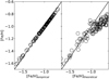 |
Fig. A.1. [Fe/H] values from Eq. (4) compared with those obtained from the empirical (left panel) and the theoretical (right panel) calibrations of Calamida et al. (2007). The solid line represents the identity relationship. |
Appendix B: Cluster metallicities
We searched the literature for metallicity estimates for the cluster sample. Because of the relatively low brightness and small angular size of some clusters, photometric estimates were more frequently found, although some low-resolution spectroscopy values and a few other high-spectroscopy ones were also found. When comparing them, we find, in some cases, a significant dispersion that is independent of the observational technique used (details are at the bottom of Table B.1), which prevented us from favoring any particular technique. In order to adopt weighted mean values, we considered the whole collection of [Fe/H] values (see Fig. 11), which allowed us to recognize a general trend and therefore to discard some visibly discrepant metallicities. We would like to note that possible sources of uncertainty due to different studies using different metallicity scales might exist.
[Fe/H] values for the cluster sample.
Appendix C: Color-color diagram of the studied clusters
Figure C.1 shows the m10 versus (v − y)0 diagrams with the positions of the selected stars in the studied LMC and SMC clusters.
All Tables
All Figures
|
Fig. 1. V vs. b − y CMD for measured stars distributed inside the star cluster’s radius (left panels) and their metallicity ([Fe/H]) distribution as a function of the V magnitude (right panels). The large filled red and blue circles represent stars used to compute the star cluster’s mean [Fe/H] value and those from a reference star field with [Fe/H] values similar to those of the star cluster’s stars, respectively (see text for details). Top and bottom panels: refer to NGC 1651 and 1795, respectively. |
| In the text | |
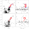 |
Fig. 2. Same as Fig. 1, for NGC 1846 (top panels) and 2155 (bottom panels). |
| In the text | |
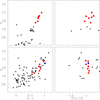 |
Fig. 3. Same as Fig. 1, for SL 8 (top panels) and 363 (bottom panels). |
| In the text | |
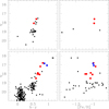 |
Fig. 4. Same as Fig. 1, for SL 388 (top panels) and 509 (bottom panels). |
| In the text | |
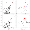 |
Fig. 5. Same as Fig. 1, for SL 549 (top panels) and 555 (bottom panels). |
| In the text | |
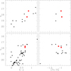 |
Fig. 6. Same as Fig. 1, for SL 817 (top panels) and 842 (bottom panels). |
| In the text | |
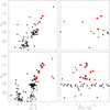 |
Fig. 7. Same as Fig. 1, for SL 862 (top panels) and L 6 (bottom panels). |
| In the text | |
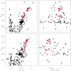 |
Fig. 8. Same as Fig. 1, for L 19 (top panels) and 27 (bottom panels). |
| In the text | |
|
Fig. 9. Individual metallicity errors as a function of the V magnitude of stars selected in a star cluster, represented by large filled red circles in Figs. 1–8. |
| In the text | |
|
Fig. 10. Ratio of the number of stars in the field and the ratio of the number of stars in the star clusters vs. the number of selected stars in each star cluster. |
| In the text | |
|
Fig. 11. Metallicity difference as a function of the star cluster’s age. Filled circles, squares, and triangles correspond to high-resolution spectroscopy, low-resolution spectroscopy, and photometry reference values, respectively. Open magenta diamonds represent metallicity differences derived from theoretical isochrones (see text for details). |
| In the text | |
|
Fig. 12. Theoretical red giant branches for log(age/yr) = 9.0 (dotted lines) and 10.10 (solid lines); [Fe/H] = −2.0, −1.5, −1.0, −0.5, and 0.0 dex shown with blue, magenta, green, orange, and red, respectively. |
| In the text | |
|
Fig. 13. Same as Fig. 11 for adopted weighted mean [Fe/H] values. The solid line represents the least squared fit obtained (see text for details). |
| In the text | |
|
Fig. A.1. [Fe/H] values from Eq. (4) compared with those obtained from the empirical (left panel) and the theoretical (right panel) calibrations of Calamida et al. (2007). The solid line represents the identity relationship. |
| In the text | |
 |
Fig. C.1. Color–color diagram of the selected stars (red filled circles in Figs. 1–8). |
| In the text | |
Current usage metrics show cumulative count of Article Views (full-text article views including HTML views, PDF and ePub downloads, according to the available data) and Abstracts Views on Vision4Press platform.
Data correspond to usage on the plateform after 2015. The current usage metrics is available 48-96 hours after online publication and is updated daily on week days.
Initial download of the metrics may take a while.