| Issue |
A&A
Volume 642, October 2020
|
|
|---|---|---|
| Article Number | L13 | |
| Number of page(s) | 5 | |
| Section | Letters to the Editor | |
| DOI | https://doi.org/10.1051/0004-6361/202039165 | |
| Published online | 09 October 2020 | |
Letter to the Editor
A perfect power-law spectrum even at the highest frequencies: The Toothbrush relic⋆
1
Dipartimento di Fisica e Astronomia, Universitát di Bologna, Via P. Gobetti 93/2, 40129 Bologna, Italy
e-mail: This email address is being protected from spambots. You need JavaScript enabled to view it.
2
INAF-Istituto di Radio Astronomia, Via Gobetti 101, 40129 Bologna, Italy
3
Thüringer Landessternwarte (TLS), Sternwarte 5, 07778 Tautenburg, Germany
4
Hamburger Sternwarte, Universität Hamburg, Gojenbergsweg 112, 21029 Hamburg, Germany
5
INAF-Osservatorio Astronomico di Cagliari, Via della Scienza 5, 09047 Selargius, CA, Italy
6
Max-Planck-Institut für Radioastronomie, Auf dem Hügel 69, 53121 Bonn, Germany
7
Leiden Observatory, Leiden University, PO Box 9513, 2300 RA Leiden, The Netherlands
Received:
12
August
2020
Accepted:
19
September
2020
Abstract
Radio relics trace shock fronts generated in the intracluster medium (ICM) during cluster mergers. The particle acceleration mechanism at the shock fronts is not yet completely understood. We observed the Toothbrush relic with the Effelsberg and Sardinia Radio Telescope at 14.25 GHz and 18.6 GHz, respectively. Unlike previously claimed, the integrated spectrum of the relic closely follows a power law over almost three orders of magnitude in frequency, with a spectral index of α58 MHz18.6 GHz = −1.16 ± 0.03. Our finding is consistent with a power-law injection spectrum, as predicted by diffusive shock acceleration theory. The result suggests that there is only little magnetic field strength evolution downstream of the shock. From the lack of spectral steepening, we find that either the Sunyaev–Zeldovich decrement produced by the pressure jump is less extended than ∼600 kpc along the line of sight or, conversely, that the relic is located far behind in the cluster. For the first time, we detect linearly polarized emission from the “brush” at 18.6 GHz. Compared to 8.3 GHz, the degree of polarization across the brush increases at 18.6 GHz, suggesting a strong Faraday depolarization toward lower frequencies. The observed depolarization is consistent with an intervening magnetized screen that arises from the dense ICM containing turbulent magnetic fields. The depolarization, corresponding to a standard deviation of the rotation measures as high as σRM = 212 ± 23 rad m−2, suggests that the brush is located in or behind the ICM. Our findings indicate that the Toothbrush relic can be consistently explained by the standard scenario for relic formation.
Key words: globular clusters: individual: 1RXS J0603.3+4213 / galaxies: clusters: intracluster medium / acceleration of particles / radiation mechanisms: non-thermal / galaxies: magnetic fields
The reduced Effelsberg Stokes I FITS file is only available at the CDS via anonymous ftp to cdsarc.u-strasbg.fr (130.79.128.5) or via http://cdsarc.u-strasbg.fr/viz-bin/cat/J/A+A/642/L13
© ESO 2020
1. Introduction
Radio relics are large, diffuse sources that are associated with powerful shock fronts originating in the intracluster medium (ICM) during cluster mergers (for a review, see e.g.,Feretti et al. 2012; van Weeren et al. 2019). One striking observational feature of radio relics is their high degree of polarization. The magnetic field vectors are often found to be well aligned with the shock surface (van Weeren et al. 2010; Bonafede et al. 2012; Owen et al. 2014; de Gasperin et al. 2014; Kierdorf et al. 2017).
Despite progress in understanding radio relics, the actual acceleration mechanism at the shock fronts is not fully understood. It is generally believed that diffusive shock acceleration (DSA; Drury 1983) generates the observed cosmic ray electrons (CRe). However, it is currently debated if the acceleration starts from the thermal pool (standard scenario; Ensslin et al. 1998; Hoeft & Brüggen 2007) or from a population of mildly relativistic electrons (re-acceleration scenario; Kang & Ryu 2011, 2016).
The standard scenario has successfully reproduced many of the observed properties of relics; however, the following three major difficulties remain: (i) the spectra of some relics are reported to show a spectral break above 10 GHz (Stroe et al. 2016), which is incompatible with the power-law spectrum predicted by DSA theory, (ii) a power-law energy distribution from the thermal pool CRe energies relevant for the synchrotron emission may require an unphysical acceleration efficiency (van Weeren et al. 2016; Botteon et al. 2020), and (iii) the Mach numbers derived from X-ray observations are often significantly lower than those derived from the overall radio spectrum (Akamatsu et al. 2012; Botteon et al. 2020).
According to the re-acceleration scenario, the shock fronts reaccelerate electrons from a pre-existing fossil population. There are a few examples, which seem to show a connection between the relic and active galactic nuclei. (Bonafede et al. 2014; van Weeren et al. 2017; Di Gennaro et al. 2018; Stuardi et al. 2019). If relics originate according to the re-acceleration scenario, weak shocks may become radio bright, solving issues (ii) and (iii). A break in the radio spectrum is expected at a high frequency, when the shock passes through a finite size cloud of a fossil electron population (Kang & Ryu 2016). If the fossil population is homogeneously distributed, the re-acceleration scenario also predicts a power-law spectrum.
The merging galaxy cluster 1RXS J0603.3+4213, located at a redshift of z = 0.225, is one of the most intriguing clusters hosting a spectacular toothbrush-shaped relic (van Weeren et al. 2012, 2016; Rajpurohit et al. 2018, 2020; de Gasperin et al. 2020). It consists of three distinct components, namely the brush (B1) and two parts forming the handle (B2+B3). The relic shows an unusual linear morphology and is quite asymmetric with respect to the merger axis. The handle extends into the very low density ICM.
Stroe et al. (2016) report evidence for a spectral steepening above 2.5 GHz in the integrated radio spectrum of the relic. This claim is mainly based on the 16 GHz and 30 GHz radio interferometric observations. It has been suggested that the steepening in the integrated radio spectrum can be reproduced with the re-acceleration scenario (Kang 2016). Basu et al. (2016) studied the impact of the Sunyaev–Zeldovich (SZ) effect on the observed synchrotron flux density. They suggest that SZ contamination leads to a high frequency steepening for relics, albeit not at the level claimed by Stroe et al. (2016). Recently, we studied the integrated spectrum of the relic between 120 MHz and 8 GHz and excluded any steepening up to 8 GHz (Rajpurohit et al. 2020). However, the spectral behavior of the relic remained uncertain between 10 and 20 GHz. The Toothbrush is known to be highly polarized (van Weeren et al. 2012). Effelsberg observations revealed a high fractional polarization at 8.3 GHz and a strong depolarization and rotation measure (RM) gradient from the brush to the handle (Kierdorf et al. 2017).
The main aim of this Letter is to answer the question if the overall spectrum of the Toothbrush steepens in the frequency range between 10−20 GHz. If the spectrum steepens at a high frequency, this would have a tremendous impact on the radio relic formation scenario, since it would clearly be in conflict with the standard scenario for relic formation, which predicts a power law toward high frequencies. A steepening would be difficult to explain within the standard scenario and would favor the re-acceleration scenario. We adopt a flat ΛCDM cosmology with H0 = 70 km s−1 Mpc−1, Ωm = 0.3, and ΩΛ = 0.7. At the cluster’s redshift, 1″ corresponds to a physical scale of 3.64 kpc.
2. Observations
The radio observations at 14.25 GHz were performed with the Effelsberg 100 m telescope with the new Ku-band receiver in dual polarization mode. The total on-source observation time was 20 h with a 2500 MHz bandwidth. We obtained 31 coverages of a field of 11 × 7 arcmin2 and processed the data with the NOD3 tool (Müller et al. 2017). The data reduction involves radio frequency interference removal and baselevel corrections, like the basket-weaving of two maps with scanning in orthogonal directions (RA/Dec).
The Sardinia Radio Telescope (SRT) observations were performed in a full polarization mode with the seven-feed K-Band receiver centered at 18.6 GHz with a bandwidth of 1200 MHz. The observations were carried out between January and February 2020, for a total of 24 h. The data were reduced using the proprietary software package Single-dish Spectral-polarimetry Software (SCUBE; Murgia et al. 2016).
The uncertainty in the flux density measurements were estimated as:
 (1)
(1)
where f is the absolute flux density calibration uncertainty, Sν is the flux density, σrms is the rms noise and Nbeams is the number of beams. We assume an absolute flux density uncertainty of 10% for both SRT and Effelsberg.
3. Results and discussion
In Fig. 1, we show the Effelsberg and the SRT total intensity images at 70″ resolution. The relic is clearly detected at both frequencies. The largest linear size of the relic is ∼1.8 Mpc, similar to the one reported below 10 GHz. We measured the flux density of 19.9 ± 3.1 mJy and 15.8 ± 3.5 mJy at 14.25 GHz and 18.6 GHz, respectively. These values are significantly higher than those reported by Stroe et al. (2016), namely S16 GHz = 10.7 ± 0.8 mJy. We speculate that the discrepancy between our measurements and the one taken by the Arcminute Microkelvin Imager interferometer is due to the “resolved-out” effects. Interferometric observations underestimate the flux density of extended emission when the size of the emission region gets close to the largest angular scale that is detectable with the interferometer.
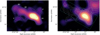 |
Fig. 1. Total power emission from the Toothbrush relic at 70″ resolution. Left: Effelsberg 14.25 GHz image. The largest linear size of the relic is ∼1.8 Mpc, similar to those reported below 10 GHz. Contour levels are drawn at |
![Mathematical equation: $ \sqrt{[1,2,4,8,\ldots]} \times 3\sigma_{\mathrm{rms}} $](/articles/aa/full_html/2020/10/aa39165-20/aa39165-20-eq3.gif)
3.1. Integrated spectrum
To obtain the integrated spectrum of the relic, we combined our new flux density measurements with those presented in Rajpurohit et al. (2020). In addition, we included the flux density measurements from the LOFAR LBA observations at 58 MHz (de Gasperin et al. 2020). We measured flux densities for the entire relic as well as for the regions B1 and B2+B3 (see Table 1).
Integrated flux densities.
The resulting integrated spectra are shown in the left panel of Fig. 2. We find that the relic follows a close power law over almost three orders of magnitude in frequency. The integrated spectral index of the relic between 58 MHz and 18.6 GHz is −1.16 ± 0.03. The spectral index value is consistent with our previous estimates (Rajpurohit et al. 2018, 2020). Recently, the power-law spectrum results are also found for the relic in CIZA J2242.8+5301 (Loi et al. 2020). The power-law spectrum is consistent with the standard scenario for the relic formation. Conversely, in the framework of the re-acceleration scenario, the absence of an upper frequency spectral break would imply that a finite size cloud of a fossil electron population is very large and distributed homogeneously. As a result, we do not see its effect in the relic’s overall spectrum.
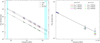 |
Fig. 2. Left: integrated spectrum of the Toothbrush relic between 58 MHz and 18.6 GHz. Dashed lines show the fitted power laws. The spectrum follows a close power law with a slope of α = −1.16 ± 0.03. The new flux density points are highlighted by the cyan regions; the other values are adopted from Rajpurohit et al. (2020). Right: possible impact of SZ decrement (shown with horizontal color lines) as a function of line of sight depth (dLOS) on the radio spectra of the relic emission. Blue circles show the observed flux densities. In order to produce an SZ decrement compatible within the error-bars of the new 14.25 and 18.6 GHz observations, the depth of the shock pressure jump along the line of sight is required to be dLOS ≤ 600 kpc. |
According to the DSA theory in the test-particle regime and adopting a constant shock strength and CRe cooling in a homogeneous medium, the “integrated” spectrum is related to the Mach number according to
 (2)
(2)
The radiative lifetime of electrons observed at 58 MHz is about 120 Myr when adopting a magnetic field strength of 1 μG. If the shock propagates with 1000 km s−1, this corresponds to length of about 160 kpc. The slope of the spectrum down to 58 MHz can only be interpreted as a Mach number, according to Eq. (2), if the physical conditions at the shock do not change significantly on a scale of 160 kpc. This condition is likely fulfilled for the Toothbrush relic, since it is located at a projected distance to the cluster center of about 1.1 Mpc. The index above, therefore, corresponds to a Mach number of ℳ = 3.7 ± 0.3.
Despite the fact that the brush is about four times brighter than the handle, the entire relic and its subregions follow a power-law behavior and show similar spectral slopes (see Table 1). At face value, this implies that the shock strength remains the same over an ∼1.8 Mpc scale. As argued in (Rajpurohit et al. 2020), the shock surface indeed shows a distribution of Mach numbers, thus a single Mach number derived above can only roughly characterize the shock. Most importantly, the tail of the Mach number distribution toward high values determine the radio spectral index (Wittor et al. 2019; Rajpurohit et al. 2020).
Our finding is basically consistent with the standard scenario for the formation of radio relics if the radio spectral index corresponds to the Mach number of the shock. If the shock would have a strength as low as estimated from the X-ray surface brightness, no radio emission that could be detected with current telescopes is expected (van Weeren et al. 2012; Botteon et al. 2020). If the shock has instead a strength as estimated from the radio spectral index, the standard DSA-based scenario is in ageement with the observations if a strong magnetic field and an efficient electron acceleration is adopted (see, e.g., Fig. 9 in Botteon et al. 2020). We note, however, that even in this situation, a few percent of the kinetic energy dissipated at the shock front needs to be transferred by DSA to the supra-thermal accelerated at the shock front.
3.2. Constraints on the downstream magnetic field evolution
It is conceivable that the magnetic field strength downstream of the shock increases, for example, due to a turbulent dynamo process driven by the curvature of the shock front, or decreases, for instance, by the expansion of the shock compressed material. Depending on frequency, the observed radio emission probes very different volumes. At the highest frequency, 50% of the emission are emitted from a volume with an extent of about 5 kpc downstream to the shock front. In contrast, the emission at 58 MHz is extended to about 85 kpc. If the strength of the magnetic field would change significantly on these length scales, this would affect the integrated spectrum of the relic.
A nonlinear change in the field strength would either significantly boost the emission at short or at large distances; in both cases, this would result in a curved spectrum (see, e.g., Donnert et al. 2016). Since the integrated spectrum almost perfectly follows a power law, only a marginal nonlinear increase or decrease in the magnetic field strength seems to be possible on scales probed by the relic.
However, if the field strength changes linearly with distance, the power-law integrated spectrum is preserved, but the relation of Eq. (2) does not hold anymore. An increasing field strength would steepen the integrated spectrum, while a decreasing one would flatten it. If the field strength doubles on a scale of 85 kpc, the spectrum would steepen by about −0.2 (the actual value depends on many parameters, e.g., the field strength itself). If the relic is formed according to the standard scenario, such a steep magnetic field gradient is clearly disfavored by the observations. A decreasing downstream field strength might be consistent with our observations, however, it would significantly aggravate the efficiency problem.
3.3. SZ decrement between 10 and 20 GHz
The SZ effect contributes a negative signal to the cosmic microwave background for ν ≤ 220 GHz. In the case of relics, Basu et al. (2016) show that the SZ effect from the shock downstream also proportionally scales the Mach number squared, producing a contamination within exactly the same spatial scales responsible for the relic emission.
At 15 GHz, the SZ effect is expected to reduce the observed synchrotron flux density by ∼10−50%, and it must be taken into account when attempting a physical interpretation in the case of any deviation from the power-law spectra. Conversely, since the SZ decrement must be expected if the shock leading to the observed relic involves thermal gas, a lack of spectral steepening can be used to further constrain the shock parameters.
The SZ decrement at a given observation frequency depends on the line-of-sight projection of the pressure jump, dLOS, and therefore on the (unknown) shock geometry at the location of the relic. For a simple plane-parallel geometry and ignoring the curvature, the total SZ decrement can be obtained by integrating y over the visible relic area: L × 𝒲, where L is the shock length and 𝒲 is the width, leading to an angular size of the relic  steradians (where DA is the angular diameter distance). Following Basu et al. (2016), we calculated the maximum total allowed SZ flux decrement from the region sampled by our new high frequency radio observation of the Toothbrush relic:
 (3)
(3)
We used DA = 751 Mpc, L = 1.86 Mpc, 𝒲 = 422 kpc, and two possible shock strengths, either ℳ = 3.7 (as suggested by radio observations) or ℳ = 1.3 (as suggested by X-ray analysis, see Ogrean et al. 2013; van Weeren et al. 2016). We note that nu and Tu are the preshock density and temperature that can be derived by the two Mach numbers, respectively. For each Mach number, the temperature and density are derived from the standard Rankine-Hugoniot jump conditions based on the assumed post-shock values, nd = 3 × 10⁻³ cm−3 and Td = 6 keV (van Weeren et al. 2016).
We thus produced estimates of  for different frequencies by fixing the above model parameters and varying the unknown value of dLOS. Our results are given in the right panel of Fig. 2. In order to produce an SZ decrement that is compatible within the error-bars of our 14.25 and 18.6 GHz observations, the depth of the shock pressure jump along the line of sight is required to be dLOS ≤ 600 kpc for a shock with a strength of ℳ = 3.7. For a shock with a strength of ℳ = 1.3, the SZ decrement at dLOS = 600 kpc already produces a spectrum that falls below the error bars of our observations. Hence, requiring an even smaller depth of the shock along the line of sight. We emphasize that the quoted values only refer to the contribution to the SZ decrement from the shock discontinuity along the line of sight for the same range of spatial scales responsible for the radio emission.
Furthermore, the assumption of a simple planar geometry and the absence of curvature along the line of sight is clearly an oversimplification, which may indeed explain the surprisingly low value of dLOS. Incidentally, such a small SZ decrement may also be explained if the shock responsible for the relic is at a more peripheral location in the cluster. In this case, the density and temperature values suggested by X-ray observations originate from regions which are denser than the one responsible for the radio emission. In this case, Eq. (3) would significantly overestimate the pressure jump at the shock, and the requirement on dLOS would be relaxed.
3.4. Polarization at 18.6 GHz
All of the information on the polarization properties of relics are mainly collected in the frequency range of 1−8.3 GHz. Since the Faraday rotation is expected to be almost negligible at 18.6 GHz, the intrinsic polarization of the relic could be directly mapped by our observations.
For the first time, we detect polarized emission from the relic at 18.6 GHz. We detect polarized emission mainly from the brush region (see Fig. 3). The degree of polarization varies along the brush and the magnetic field vectors are mainly aligned to the relic’s orientation. The fractional polarization reaches ∼66% in some areas, the average being ∼30 ± 7%. We note that these values could be affected by beam depolarization.
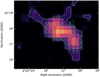 |
Fig. 3. B-vectors distribution across the brush region at 51″ resolution overlaid with the SRT total power contours at 3σ. The length of the vectors depict the degree of polarization. The vectors are corrected for Faraday rotation effect. The mean polarization fraction at the brush is (30 ± 7)%. |
Previous polarization measurements of the Toothbrush relic have shown that the fractional polarization of B1 decreases rapidly toward lower frequencies. B1 is polarized at a level of about 15% at 8.3 GHz (Kierdorf et al. 2017) and about 11% at 4.9 GHz. The polarization fraction drops below 1% at a frequency near 1.4 GHz (van Weeren et al. 2012). The comparison between 8.3 GHz and our measurement suggests significant depolarization even between 18.6 and 8.3 GHz. Other than the Toothbrush relic, the polarization observations above 4.9 GHz are only available for three relics, namely the Sausage relic, the relic in ZwCl 0008+52, and Abell 1612 (Kierdorf et al. 2017; Loi et al. 2017). For the above mentioned relics, the fractional polarization remains nearly constant at 4.9 GHz and 8.3 GHz.
The standard deviation of the RM, σRM, is a useful parameter to characterize Faraday rotation and depolarization caused by an external Faraday screen. The depolarization induced by an external Faraday screen containing turbulent magnetic fields (Burn 1966; Sokoloff et al. 1998) can be described as
 (4)
(4)
where p0 is the intrinsic polarization fraction. The maps between 4.9 and 18.6 GHz show depolarization of  for B1. This enabled us to derive σRM = 212 ± 23 rad m−2. The observed σRM for the brush is several times higher than for any other radio relic. This indicates that the brush region of the relic experiences Faraday rotation strongly from the dense ICM. The strong depolarization suggests that the emission lies in or behind the ICM, which very likely causes a low Mach number shock detected via X-ray observations (Ogrean et al. 2013; van Weeren et al. 2016).
4. Conclusions
We presented high frequency radio observations of the Toothbrush relic with the SRT and the Effelsberg telescope. We find that the relic follows a close power-law spectrum between 58 MHz and 18.6 GHz, with a slope of α = −1.16 ± 0.03. Our findings indicate that Toothbrush can be consistently explained by the standard scenario for relic formation. The slope of the spectrum disfavors that the strength of the magnetic field significantly changes on scales probed by the radio emission, that is to say about 85 kpc.
We detected polarized emission at 18.6 GHz. Compared to measurements at lower frequencies, the polarization fraction of the brush increases at 18.6 GHz. The high value of σRM is consistent with σRM fluctuations of an ICM screen with tangled magnetic fields. This suggests that the brush is located in or behind the ICM.
From the lack of steepening in the relic spectra, we find that either the SZ decrement at the shock along the line of sight is ≤600 kpc thick, or the pressure jump associated with the relic is located far behind in the cluster. The latter explanation can also be reconciled with the trends of the polarization fraction for the brush region.
Acknowledgments
KR and FV acknowledge financial support from the ERC Starting Grant “MAGCOW”, no. 714196. FL acknowledge financial support from the Italian Minister for Research and Education (MIUR), project FARE, project code R16PR59747, project name FORNAX-B. RJvW acknowledges support from the VIDI research programme with project number 639.042.729, which is financed by the Netherlands Organisation for Scientific Research (NWO). CJR and EB acknowledges financial support from the ERC Starting Grant “DRANOEL” number 714245. AD acknowledges support by the BMBF Verbundforschung under grant 05A17STA. We thank Sorina Reile for processing part of the Effelsberg data. Based on observations with the 100 m telescope of the MPIfR (Max-Planck-Institut für Radioastronomie) at Effelsberg. The Sardinia Radio Telescope (Bolli et al. 2015; Prandoni et al. 2017) is funded by the Ministry of Education, University and Research (MIUR), Italian Space Agency (ASI), the Autonomous Region of Sardinia (RAS) and INAF itself and is operated as National Facility by the National Institute for Astrophysics (INAF). The development of the SARDARA back-end has been funded by the Autonomous Region of Sardinia (RAS) using resources from the Regional Law 7/2007 “Promotion of the scientific research and technological innovation in Sardinia”.
References
- Akamatsu, H., Takizawa, M., Nakazawa, K., et al. 2012, PASJ, 64, 67 [NASA ADS] [Google Scholar]
- Basu, K., Vazza, F., Erler, J., & Sommer, M. 2016, A&A, 591, A142 [NASA ADS] [CrossRef] [EDP Sciences] [Google Scholar]
- Bolli, P., Orlati, A., Stringhetti, L., et al. 2015, J. Astron. Instrum., 4, 1550008 [CrossRef] [Google Scholar]
- Bonafede, A., Brüggen, M., van Weeren, R., et al. 2012, MNRAS, 426, 40 [NASA ADS] [CrossRef] [Google Scholar]
- Bonafede, A., Intema, H. T., Brüggen, M., et al. 2014, ApJ, 785, 1 [NASA ADS] [CrossRef] [Google Scholar]
- Botteon, A., Brunetti, G., Ryu, D., & Roh, S. 2020, A&A, 634, A64 [NASA ADS] [CrossRef] [EDP Sciences] [Google Scholar]
- Burn, B. J. 1966, MNRAS, 133, 67 [NASA ADS] [CrossRef] [Google Scholar]
- de Gasperin, F., van Weeren, R. J., Brüggen, M., et al. 2014, MNRAS, 444, 3130 [NASA ADS] [CrossRef] [Google Scholar]
- de Gasperin, F., Brunetti, G., Bruggen, M., et al. 2020, A&A, 642, A85 [CrossRef] [EDP Sciences] [Google Scholar]
- Di Gennaro, G., van Weeren, R. J., Hoeft, M., et al. 2018, ApJ, 865, 24 [NASA ADS] [CrossRef] [Google Scholar]
- Donnert, J. M. F., Stroe, A., Brunetti, G., Hoang, D., & Roettgering, H. 2016, MNRAS, 462, 2014 [NASA ADS] [CrossRef] [Google Scholar]
- Drury, L. O. 1983, Rep. Prog. Phys., 46, 973 [NASA ADS] [CrossRef] [Google Scholar]
- Ensslin, T. A., Biermann, P. L., Klein, U., & Kohle, S. 1998, A&A, 332, 395 [NASA ADS] [Google Scholar]
- Feretti, L., Giovannini, G., Govoni, F., & Murgia, M. 2012, A&ARv, 20, 54 [Google Scholar]
- Hoeft, M., & Brüggen, M. 2007, MNRAS, 375, 77 [NASA ADS] [CrossRef] [Google Scholar]
- Kang, H. 2016, J. Korean Astron. Soc., 49, 83 [CrossRef] [Google Scholar]
- Kang, H., & Ryu, D. 2011, ApJ, 734, 18 [NASA ADS] [CrossRef] [Google Scholar]
- Kang, H., & Ryu, D. 2016, ApJ, 823, 13 [NASA ADS] [CrossRef] [Google Scholar]
- Kierdorf, M., Beck, R., Hoeft, M., et al. 2017, A&A, 600, A18 [NASA ADS] [CrossRef] [EDP Sciences] [Google Scholar]
- Loi, F., Murgia, M., Govoni, F., et al. 2017, MNRAS, 472, 3605 [NASA ADS] [CrossRef] [Google Scholar]
- Loi, F., Murgia, M., Vacca, V., et al. 2020, MNRAS, 498, 1628 [CrossRef] [Google Scholar]
- Müller, P., Krause, M., Beck, R., & Schmidt, P. 2017, A&A, 606, A41 [NASA ADS] [CrossRef] [EDP Sciences] [Google Scholar]
- Murgia, M., Govoni, F., Carretti, E., et al. 2016, MNRAS, 461, 3516 [NASA ADS] [CrossRef] [Google Scholar]
- Ogrean, G. A., Brüggen, M., van Weeren, R. J., et al. 2013, MNRAS, 433, 812 [NASA ADS] [CrossRef] [Google Scholar]
- Owen, F. N., Rudnick, L., Eilek, J., et al. 2014, ApJ, 794, 24 [NASA ADS] [CrossRef] [Google Scholar]
- Prandoni, I., Murgia, M., Tarchi, A., et al. 2017, A&A, 608, A40 [NASA ADS] [CrossRef] [EDP Sciences] [Google Scholar]
- Rajpurohit, K., Hoeft, M., van Weeren, R. J., et al. 2018, ApJ, 852, 65 [NASA ADS] [CrossRef] [Google Scholar]
- Rajpurohit, K., Hoeft, M., Vazza, F., et al. 2020, A&A, 636, A30 [CrossRef] [EDP Sciences] [Google Scholar]
- Sokoloff, D. D., Bykov, A. A., Shukurov, A., et al. 1998, MNRAS, 299, 189 [NASA ADS] [CrossRef] [Google Scholar]
- Stroe, A., Shimwell, T., Rumsey, C., et al. 2016, MNRAS, 455, 2402 [NASA ADS] [CrossRef] [Google Scholar]
- Stuardi, C., Bonafede, A., Wittor, D., et al. 2019, MNRAS, 489, 3905 [NASA ADS] [Google Scholar]
- van Weeren, R. J., Röttgering, H. J. A., Brüggen, M., & Hoeft, M. 2010, Science, 330, 347 [NASA ADS] [CrossRef] [PubMed] [Google Scholar]
- van Weeren, R. J., Röttgering, H. J. A., Intema, H. T., et al. 2012, A&A, 546, A124 [NASA ADS] [CrossRef] [EDP Sciences] [Google Scholar]
- van Weeren, R. J., Brunetti, G., Brüggen, M., et al. 2016, ApJ, 818, 204 [NASA ADS] [CrossRef] [Google Scholar]
- van Weeren, R. J., Andrade-Santos, F., Dawson, W. A., et al. 2017, Nat. Astron., 1, 0005 [NASA ADS] [CrossRef] [Google Scholar]
- van Weeren, R. J., de Gasperin, F., Akamatsu, H., et al. 2019, Space Sci. Rev., 215, 16 [NASA ADS] [CrossRef] [Google Scholar]
- Wittor, D., Hoeft, M., Vazza, F., Brüggen, M., & Domínguez-Fernández, P. 2019, MNRAS, 490, 3987 [NASA ADS] [CrossRef] [Google Scholar]
All Tables
All Figures
|
Fig. 1. Total power emission from the Toothbrush relic at 70″ resolution. Left: Effelsberg 14.25 GHz image. The largest linear size of the relic is ∼1.8 Mpc, similar to those reported below 10 GHz. Contour levels are drawn at |
| In the text | |
|
Fig. 2. Left: integrated spectrum of the Toothbrush relic between 58 MHz and 18.6 GHz. Dashed lines show the fitted power laws. The spectrum follows a close power law with a slope of α = −1.16 ± 0.03. The new flux density points are highlighted by the cyan regions; the other values are adopted from Rajpurohit et al. (2020). Right: possible impact of SZ decrement (shown with horizontal color lines) as a function of line of sight depth (dLOS) on the radio spectra of the relic emission. Blue circles show the observed flux densities. In order to produce an SZ decrement compatible within the error-bars of the new 14.25 and 18.6 GHz observations, the depth of the shock pressure jump along the line of sight is required to be dLOS ≤ 600 kpc. |
| In the text | |
|
Fig. 3. B-vectors distribution across the brush region at 51″ resolution overlaid with the SRT total power contours at 3σ. The length of the vectors depict the degree of polarization. The vectors are corrected for Faraday rotation effect. The mean polarization fraction at the brush is (30 ± 7)%. |
| In the text | |
Current usage metrics show cumulative count of Article Views (full-text article views including HTML views, PDF and ePub downloads, according to the available data) and Abstracts Views on Vision4Press platform.
Data correspond to usage on the plateform after 2015. The current usage metrics is available 48-96 hours after online publication and is updated daily on week days.
Initial download of the metrics may take a while.