| Issue |
A&A
Volume 648, April 2021
|
|
|---|---|---|
| Article Number | A46 | |
| Number of page(s) | 19 | |
| Section | Celestial mechanics and astrometry | |
| DOI | https://doi.org/10.1051/0004-6361/202040269 | |
| Published online | 09 April 2021 | |
Relativistic modeling of atmospheric occultations with time transfer functions
1
Dipartimento di Ingegneria Industriale, Alma Mater Studiorum – Università di Bologna,
Via Fontanelle 40,
47121
Forlì, Italy
e-mail: This email address is being protected from spambots. You need JavaScript enabled to view it.
2
Interdepartmental Center for Industrial Research in Aerospace (CIRI AERO), Alma Mater Studiorum – Università di Bologna,
Via B. Carnaccini 12,
47121
Forlì, Italy
3
SYRTE, Observatoire de Paris, Université PSL, CNRS, Sorbonne Université, LNE,
61 avenue de l’Observatoire,
75014
Paris, France
Received:
31
December
2020
Accepted:
26
February
2021
Abstract
Context. Occultation experiments represent unique opportunities to remotely probe the physical properties of atmospheres. The data processing involved in modeling the time and frequency transfers of an electromagnetic signal requires that refractivity be properly accounted for. On theoretical grounds, little work has been done concerning the elaboration of a covariant approach for modeling occultation data.
Aims. We present an original method allowing fully analytical expressions to be derived up to the appropriate order for the covariant description of time and frequency transfers during an atmospheric occultation experiment.
Methods. We make use of two independent powerful relativistic theoretical tools, namely the optical metric and the time transfer functions formalism. The former allows us to consider refractivity as spacetime curvature while the latter is used to determine the time and frequency transfers occurring in a curved spacetime.
Results. We provide the integral form of the time transfer function up to any post-Minkowskian order. The discussion focuses on the stationary optical metric describing an occultation by a steadily rotating and spherically symmetric atmosphere. Explicit analytical expressions for the time and frequency transfers are provided at the first post-Minkowskian order and their accuracy is assessed by comparing them to results of a numerical integration of the equations for optical rays.
Conclusions. The method accurately describes vertical temperature gradients and properly accounts for the light-dragging effect due to the motion of the optical medium. It can be pushed further in order to derive the explicit form of the time transfer function at higher order and beyond the spherical symmetry assumption.
Key words: atmospheric effects / methods: analytical / occultations / planets and satellites: atmospheres / relativistic processes
© ESO 2021
1 Introduction
Theoretical problems dealing with time and frequency transfers require knowledge of the function relating the (coordinate) time transfer to the coordinate time at reception and to the spatial coordinates of the reception and emission point-events. Such a function is called a reception time transfer function. An emission time transfer function can be introduced too. The formalism designed to determine the time transfer functions is called the time transfer functions formalism. It was first introduced by Linet & Teyssandier (2002) relying on the theory of the world function developed by Synge (1960). Later on a general post-Minkowskian expansion of the world and the time transfer functions was proposed by Le Poncin-Lafitte et al. (2004) and then the method was refined by Teyssandier & Le Poncin-Lafitte (2008) thanks to a simplified iterative procedure. The time transfer functions formalism confers a great advantage in that it spares the trouble of integrating the geodesic equation, which usually leads to heavy calculations, especially beyond the post-Minkowskian regime (Richter & Matzner 1983; Brumberg 1987). Until recently, the time transfer functions formalism was systematically applied to the physical spacetime considering only gravitational effects on a ray of light propagating in a vacuum. However, Bourgoin (2020) showed that theoretical problems dealing with optical rays propagating into flowing dielectric medium could also be solved making use of the time transfer functions formalism by means of a powerful theoretical tool known as the optical metric or the Gordon’s metric of spacetime.
When a ray of light is propagating into an optical medium its trajectory does not follow a null geodesic path of the physical spacetime because light and matter interact. Conventionally, the real trajectory is therefore determined by solving Maxwell’s equation within the framework of geometrical optics. However, another interesting possibility initially proposed by Gordon (1923) is to introduce an artificial optical metric which implicitly accounts for the interaction between light and matter such that optical rays follow null geodesics of that new optical metric. In other words, refractivity is treated as spacetime curvature in the optical metric. Therefore, the time and frequency transfers can still be determined with the time transfer functions formalism even when considering a ray of light crossing through an optical medium.
Occultation experiments are an example of an observing technique requiring careful treatment of refractivity while modeling the time and frequency transfers. The method consists in remotely measuring the physical properties of a planetary atmosphere while the source of an electromagnetic signal is being occulted by the atmosphere. When the source is a radio signal emitted by a spacecraft’s antenna the experiment is called an atmospheric radio occultation (Kliore et al. 1965; Fjeldbo & Eshleman 1965, 1968; Lindal et al. 1985, 1987; Lindal 1992; Schinder et al. 2012, 2015), whereas it is called an atmospheric stellar occultation when the source is made of visible or near-infrared light emitted by a distant star (Roques et al. 1994; Sicardy et al. 2006). In practice, two methods are usually employed for processing occultation data, namely the Abel inversion for spherical symmetry (Phinney & Anderson 1968; Steiner et al. 1999) and the numerical ray-tracing for any generic case (Schinder et al. 2015). The former is an exact expression providing the index of the refraction profile directly from the bending angle which is itself retrieved from the frequency transfer. The latter consists in a numerical integration of the equations for optical rays across a layered atmosphere. The refractivity in each layer and the initial pointing direction are iteratively determined such that the computed frequency coincides with the observed frequency. While the numerical ray-tracing method is the most general one, it does not provide a comprehensive description of the light path and requires significant computational time. On the other hand, if the Abel inversion method does not require numerically solving for the equations for optical rays, it can only be applied to spherically symmetric atmospheres and cannot account for the atmospheric time delay which eventually affects the determination of the emitter’s position (i.e., the spacecraft in a one-way downlink configuration during a radio occultation event). In addition, as in numerical ray-tracing, the Abel inversion does not provide a comprehensive description of the light path. An analytical expression describing the time and frequency transfers for radio occultation experiments would allow these issues to be overcome.
With this goal in mind, Bourgoin et al. (2019) proposed a new approach exploiting similarities between equations of geometrical optics and equations of celestial mechanics. It consists in expressing the equations of geometrical optics as a set of first-order perturbation equations (similar to Gauss equations of celestial mechanics) which are better suited for finding analytical solutions beyond the spherical symmetry assumption. However, even if the perturbation equations can be solved more easily than the equations of geometrical optics it is still a challenging task to solve for the second-order expressions or to incorporate the light-dragging effect caused by the motion of the optical medium.
In this paper, we make use of the time transfer functions formalism considering an optical metric in order to accurately model the time and frequency transfers for occultation experiments involving a flowing spherically symmetric atmosphere. The determination of the time transfer functions allows us to account for the atmospheric time delay. In addition, the formalism being fully covariant, it naturally accounts for the light-dragging effect due to the motion of the optical medium and constitutes in that sense a significant improvement with respect to the perturbation equations approach.
The paper is organized as follows. Section 2 lists the notations and assumptions we make throughout the paper. Section 3 recalls some basic information about relativistic geometrical optics and allows us to define the index of refraction, the refractivity, and the optical metric. The equations for optical rays propagating in an isotropic dispersive medium are derived in the same section. The reader who is already familiar with relativistic geometrical optics can skip this section. Section 4 recalls basic information about the time transfer functions formalism and introduces the refractive delay function and the post-Minkowskian parameter N0. The integral form of the delay function is given at any post-Minkowskian order. Section 5 is an application to occultation experiments involving steadily rotating and spherically symmetric atmospheres. The refractivity profile is built in Sect. 6 considering an exponential pressure profile and a polynomial temperature profile of arbitrary degree. The refractive delay function is finally solved at first post-Minkowskian order in the limit where the angular velocity of the optical medium is small with respect to the speed of light in a vacuum. The expressions for the time and frequency transfers are given explicitly. Section 7 assesses the accuracy of the first-order solutions for the time and frequency transfers by comparing them to results of a numerical integration of the equations for optical rays propagating into a nondispersive isotropic medium. Finally, we give our conclusions in Sect. 8. Appendix A is a discussion about the Abel transform method for finding the refractivity from the frequency transfer while considering the light-dragging effect.
2 General assumptions and notations
In this paper, the influence of gravity on the propagation of light is regarded as negligible, and so the physical metric g of spacetime is assumed to be a Minkowski metric. Greek indices run from 0 to 3, and Latin indices run from 1 to 3. We systematically make use of an orthonormal Cartesian coordinate system (xμ) = (x0, xi), and so the components of the physical metric may be written as
 (1)
(1)
where
 (2)
(2)
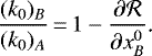
We put x0 = ct, with c being the speed of light in a vacuum and t a time coordinate, and we use x to denote the triplet of spatial coordinates (x1, x2, x3). More generally, we use the notation a = (ai) = (a1, a2, a3) for a triplet constituted by the spatial components of a 4-vector, and  for a triplet built with the spatial components of a covariant 4-vector.
Given the triplet a, b, and  , the usual Euclidean scalar product a ⋅b is denoted aibi = δikaibk, where δik is the Kronecker delta. Similarly,
  denotes the quantity aici = δikaick. In each case, Einstein’s summation convention on repeated indices is used. Furthermore, ∥a∥ denotes the Euclidean norm of a:
  . Similarly,
  denotes the quantity
  .
.
For the sake of legibility, we employ  or
or ![Mathematical equation: $[f]_{x}$](/articles/aa/full_html/2021/04/aa40269-20/aa40269-20-eq10.png) instead of f(x) whenever necessary. When a quantity f(x) is to be evaluated at two point-events xA and xB, we employ
instead of f(x) whenever necessary. When a quantity f(x) is to be evaluated at two point-events xA and xB, we employ  to denote f(xA) and f(xB), respectively. The partial differentiation of f with respect to xμ is denoted ∂μf or f,μ.
3 Relativistic geometrical optics
This paper is devoted to the propagation of light rays through a linear, isotropic, and nondispersive medium filling a spatially bounded region  in Minkowski spacetime. The region exterior to
  is assumed to be empty of any matter. According to these assumptions, the basic relations of the present paper are inferred by substituting the metric components gμν from Eq. (1) into the equations supplied in Bourgoin (2020).
The electromagnetic properties of the medium are characterized by two scalar functions, the permittivity ϵ(x) and the permeability μ(x). The index of refraction of the medium is the scalar function defined by the well-known relationship
 (3)
(3)
Moreover, it is assumed that the medium is made of a fluid schematized by a flow of particles which are not colliding. The unit 4-velocity vector of a particle of the fluid at a point-event x of its world-line is denoted wμ(x). Outside  , the permittivity and the permeability reduce to their vacuum values ϵ(x) = ϵ0 and μ(x) = μ0, respectively. As
  , the index of refraction then reduces to n(x) = 1. The expression for the refractivity is obtained by subtracting its vacuum value from the index of refraction, namely
 (4)
(4)
In the context of the geometrical optics approximation, the light rays propagating through our medium are the bicharacteristic curves of the so-called eikonal equation, which reads
 (5)
(5)
where  is the eikonal function and ḡμν is the contravariant tensor defined by
 (6)
(6)
Let us use ḡμν to denote the quantities such that
 (7)
(7)
An elementary calculation leads to
 (8)
(8)
The quantities ḡμν can be regarded as the components of a Lorentzian metric ḡ defined on the region  . This new metric is called the optical metric associated with the optical medium, terminology justified by the following considerations, which were derived by Gordon (1923), Quan (1957), and Ehlers (1967).
Let us define the 4-wave covector field kμ as
 (9)
(9)
A contravariant vector field kμ can be associated with this covector by putting
 (10)
(10)
As recalled by Bourgoin (2020), it is convenient to define the contravariant vector field  as
as
 (11)
(11)
Indeed, the light rays xμ = xμ(ζ) associated with a solution  of the eikonal Eq. (5) are the integral curves of the vector field
  , namely, they are solutions of the differential system (Perlick 2000)
 (12)
(12)
A classical calculation shows that the solutions of Eq. (12) are null geodesics of the optical metric ḡ (Synge 1960; Perlick 2000), ζ being an affine parameter. The null character of the rays is directly inferred from Eqs. (7), (12), and (5). We have indeed:
 (13)
(13)
The eikonal Eq. (5) is the Jacobi equation associated with the Hamiltonian
 (14)
(14)
where kν must be regarded as conjugate canonical variables of xμ. As a consequence, the light rays in the region  can be considered as solutions of the set of canonical equations (Quan 1957)

It must be noted that the eikonal function is constant along a light ray. Indeed, it follows from Eqs. (12) and (13) that
 (16)
(16)
This property is at the core of the procedure developed in the following section.
For numerical integration, it is relevant to separate space and time components in Eq. (15). Let li be the components defined by
 (17)
(17)
and let ℓ be a new parametrization of the curves for optical rays (Schinder et al. 2015) such that
 (18)
(18)
After inserting these new quantities into the set of canonical Eq. (15), we find for the time components:
![Mathematical equation: \begin{align*} \frac{\textrm{d} x^0}{\textrm{d}\ell}\;{=}&\;\frac{1}{n}\left[1+(n^2-1)\left(w^0+w^kl_k\right)w^0\right]\text{,}\\ \frac{\textrm{d}\ln\Vert k_0\Vert}{\textrm{d}\ell}\;{=}&\;-n_{,0}\left(w^0+w^kl_k\right)^2\nonumber\\ &-\frac{(n^2-1)}{n}\left(w^0+w^kl_k\right)\left(w^0_{\,0}+w^k_{\,0}l_k\right)\text{,}\end{align*}](/articles/aa/full_html/2021/04/aa40269-20/aa40269-20-eq38.png)
and, for the space components:
![Mathematical equation: \begin{align*} \frac{\textrm{d} x^i}{\textrm{d}\ell}\;{=}&\;{-}\frac{1}{n}\left[l_i-(n^2-1)\left(w^0+w^kl_k\right)w^i\right]\text{,}\\ \frac{\textrm{d} l_i}{\textrm{d}\ell}\;{=}&\;{-}n_{,i}\left(w^0+w^kl_k\right)^2\nonumber\\ &-\frac{(n^2-1)}{n}\left(w^0+w^kl_k\right)\left(w^0_{\,i}+w^k_{\,i}l_k\right)-\frac{\textrm{d}\ln\Vert k_0\Vert}{\textrm{d}\ell}l_i\text{.} \end{align*}](/articles/aa/full_html/2021/04/aa40269-20/aa40269-20-eq39.png)
Equations (19) may be particularly interesting in the case where the index of refraction n and the unit 4-velocity wμ do not depend on time, and we use them in our attempt at numerical integration (see Sect. 7). It is worthy of note that in this case the component k0 is constant along each light ray.
4 Refractive delay function
In this section, we introduce the formalism of time transfer functions that we apply to optical metric in order to describe refraction due to a linear, isotropic, and nondispersive medium.
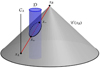 |
Fig. 1 Illustration of an occultation event in spacetime. The past light cone
|


4.1 Timetransfer functions formalism
Let us consider a light ray ΓAB starting from an emission point-event  and arriving at a reception point-event
  . We consider that a part of ΓAB travels through the domain
  , while the other part travels through a vacuum, that is a medium such that n = 1 (see Fig. 1).
It is immediately inferred from Eq. (16) that the phase  is constant along ΓAB. As a consequence, the coordinates of the emission point xA and of the reception point xB are such that the following relation is satisfied:
 (20)
(20)
Equation (20) shows that  may be considered as an implicit function of xA and the coordinates of the reception point, namely
  and xB. Hence, it is appropriate to introduce
  the reception time transfer function associated with ΓAB as
 (21)
(21)
An emission time transfer function can be introduced too. Hereafter, we merely consider the case at reception which is better suited for a downlink one-way transfer during an occultation event with a radio signal that is recorded when received.
A relevant theorem about the components of the 4-wave covector can be directly inferred from Eqs. (20) and (21); see Le Poncin-Lafitte et al. (2004). Indeed after writing Eq. (21) as
 (22)
(22)
and then inserting this relation into Eq. (20), we get the following expression:
 (23)
(23)
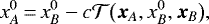
Equation (23) is in fact an identity. Therefore, straightforward differentiations of this last relation with respect to xA,  , and xB lead to the following set of equations:
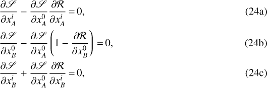
where we introduced  a reception range transfer function as
 (25)
(25)
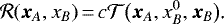
Using Eqs. (9) and (17), it is easily seen that Eq. (24) imply the following relationships:

and
 (26c)
(26c)
Unsurprisingly, these relations are similar to Eqs. (40)–(42) of Le Poncin-Lafitte et al. (2004) established for optical rays in a vacuum. We actually see that they are still valid for optical rays propagating into a linear, isotropic, and nondispersive medium within the framework of geometrical optics.
The main interest of Eq. (26) lies in the fact that it enables us to calculate the Doppler effect between an emitter and a receiver when the explicit expression of the function  is known. Indeed, it is well known (Synge 1960; Blanchet et al. 2001) that the Doppler frequency shift measured between an emitter and a receiver can be expressed as
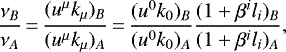 (27)
(27)
where  are the unit 4-velocity vectors of the emitter and receiver defined by
 (28)
(28)
with
 (29)
(29)
The unit 4-velocity is by definition a unit vector for the physical metric of spacetime Eq. (1), hence
 (30)
(30)
where  denote the coordinate 3-velocity vectors of the emitter and receiver, namely
 (31)
(31)
As shown by Linet & Teyssandier (2002) and Hees et al. (2012, 2014), the frequency transfer may be expressed in terms of the time (orsimilarly the range) transfer function after inserting Eqs. (26) and (30) into (27), namely
 (32)
(32)
with

Therefore, the time and frequency transfers in Eqs. (21) and (33) can be computed once the explicit form of the time (or similarly the range) transfer function is known.
The time transfer function may be determined from the eikonal equation. Indeed, after making use of Eq. (9) and (17) while evaluating Eq. (5) at xA, we end up with
 (34)
(34)
Then, by invoking Eqs. (26), (6), and assumption (1), we obtain the Hamilton-Jacobi equation that is satisfied by  . By replacing xA by a variable x while considering
  and xB as fixed parameters, the Hamilton-Jacobi equation eventually reads
![Mathematical equation: \begin{align*} \big[\partial_i\mathcal R\,\partial_i\mathcal R\big]_{(\bm{x},x_B)}\;{=}&\;1+\kappa^{00}\big(x_B^0-\mathcal R\big(\bm{x},x_B\big),\bm{x}\big)\nonumber\\ &+2\kappa^{0i}\big(x_B^0-\mathcal R\big(\bm{x},x_B\big),\bm{x}\big)\big[\partial_i\mathcal R\big]_{(\bm{x},x_B)}\nonumber\\ &+\kappa^{ij}\big(x_B^0-\mathcal R\big(\bm{x},x_B\big),\bm{x}\big)\big[\partial_i\mathcal R\,\partial_j\mathcal R\big]_{(\bm{x},x_B)}\text{.}\end{align*}](/articles/aa/full_html/2021/04/aa40269-20/aa40269-20-eq70.png) (35)
(35)
The form of the optical metric in Eqs. (6) and (8) implies that the range transfer function can be looked for as
 (36)
(36)
where Δ is a refractive delay function. In the present context, the delay function depends on κμν and is due to refraction when the light ray is crossing through  . After substituting
  from Eqs. (36) into (35), we find the following expression:
![Mathematical equation: \begin{equation*} -2N^i\big[\partial_i\Delta\big]_{(\bm{x},x_B)}\,{=}\,W(x,x_B)\text{,}\end{equation*}](/articles/aa/full_html/2021/04/aa40269-20/aa40269-20-eq74.png) (37)
(37)
where we introduced
![Mathematical equation: \begin{align*} W(x,x_B)\;{=}&\;\big(\kappa^{00}-2\kappa^{0i}N^i+\kappa^{ij}N^iN^j\big)_x\nonumber\\ &+2\big(\kappa^{0i}-\kappa^{ij}N^j\big)_x\big[\partial_i\Delta\big]_{(\bm{x},x_B)}\nonumber\\ &+\big(\kappa^{ij}-\delta^{ij}\big)_x\big[\partial_i\Delta\,\partial_j\Delta\big]_{(\bm{x},x_B)}\text{,} \end{align*}](/articles/aa/full_html/2021/04/aa40269-20/aa40269-20-eq75.png) (38)
(38)
with N given by
 (39)
(39)
and where the point-event x is defined as
 (40)
(40)
As x is a free variable, we choose for convenience to consider the case where x is varying along the straight line segment joining xA and xB, that is x = z(σ) with
 (41)
(41)
where RAB = ∥xB −xA∥. In that respect, we have
 (42)
(42)
A straightforward calculation shows that the total differentiation of Δ(z(σ), xB) with respect to σ is given by
![Mathematical equation: \begin{equation*} \frac{\textrm{d}}{\textrm{d}\sigma}\Delta\big(\bm{z}(\sigma),x_B\big)\,{=}\,{-}R_{AB}N_{AB}^i\big[\partial_i\Delta\big]_{(\bm{z}(\sigma),x_B)}\text{,}\end{equation*}](/articles/aa/full_html/2021/04/aa40269-20/aa40269-20-eq80.png) (43)
(43)
where ![Mathematical equation: $[\partial_i\Delta]_{(\bm{z}(\sigma),x_B)}$](/articles/aa/full_html/2021/04/aa40269-20/aa40269-20-eq81.png) denotes the partial derivative of Δ(x, xB) with respect to xi taken at x = z(σ). Then, after inserting Eqs. (37) and (39) into (43) while accounting for Eq. (42), we infer
denotes the partial derivative of Δ(x, xB) with respect to xi taken at x = z(σ). Then, after inserting Eqs. (37) and (39) into (43) while accounting for Eq. (42), we infer
 (44)
(44)
where the components of the point-event  are given by (40) with
  , namely
 (45)
(45)
Equation (44) is the fundamental differential equation for the determination of the delay function, and can be integrated with the following boundary conditions

which follow from the requirement that Δ(xB, xB) = 0 and from z(0) = xB. Therefore, Eq. (44) is such that
![Mathematical equation: \begin{align*} \Delta(\bm{x}_A,x_B)\;{=}&\;\frac{R_{AB}}{2}\int_{\mathcal D}\bigg\{\big(\kappa^{00}-2\kappa^{0i}N^i_{AB}+\kappa^{ij}N^i_{AB}N^j_{AB}\big)_{\tilde z(\sigma)}\nonumber\\ &+2\big(\kappa^{0i}-\kappa^{ij}N_{AB}^j\big)_{\tilde z(\sigma)}\left[\partial_i\Delta\right]_{(\bm{z}(\sigma),x_B)}\bigg.\nonumber\\ &-\left[\partial_i\Delta\,\partial_i\Delta\right]_{(\bm{z}(\sigma),x_B)}\bigg\}\,\textrm{d}\sigma\text{,}\end{align*}](/articles/aa/full_html/2021/04/aa40269-20/aa40269-20-eq87.png) (47)
(47)
where the integration goes from σ = 0 to 1 and is limited to the spacetime region within  .
.
4.2 Post-Minkowskian expansion
As we plan to apply our general formalism to occultation measurements, we suppose that the refractivity of the medium satisfies the condition
 (48)
(48)
on the domain  . This condition implies that the optical metric ḡ deviates only slightly from the Minkowski metric, namely
 (49)
(49)
It will be convenient to use the maximum value N0 of the refractivity as a small parameter. For a rocky planet or satellite, N0 can be defined as the refractivity at ground level. For gas giants, N0 can be defined as the refractivity at a certain pressure level. In each case, we can put
 (50)
(50)
where  at each point
  . With this definition of
  , the perturbation terms in the optical metric read
 (51a)
(51a)
with
 (51b)
(51b)
Our modeling is based on the two following additional assumptions: (i) the function  is independent of N0, and (ii) the spatial positions of the emitter and of the receiver are such that the light ray ΓAB, which can be observed in realistic situations, has a delay function Δ(xA, xB) given by the expansion
 (52)
(52)
Inserting the expansions (51) and (52) into (47), one deduces the expressions for the quantities Δ(m) as (Bourgoin 2020)
![Mathematical equation: \begin{align} \Delta^{(1)}(\bm{x}_A,x_B)\;{=}&\;\frac{R_{AB}}{2}\nonumber\\ &\times\int_{\mathcal D}\left(\kappa^{00}_{(1)}-2\kappa^{0i}_{(1)}N^i_{AB}+\kappa^{ij}_{(1)}N^i_{AB}N^j_{AB}\right)_{z(\sigma)}\textrm{d}\sigma\text{,}\\ \Delta^{(2)}(\bm{x}_A,x_B)\;{=}&\;\frac{R_{AB}}{2}\int_{\mathcal D}\Bigg\{\left(\hat{\kappa}^{00}_{(2)}-2\hat{\kappa}^{0i}_{(2)}N^i_{AB}+\hat{\kappa}^{ij}_{(2)}N^i_{AB}N^j_{AB}\right)_{(z(\sigma),x_B)}\nonumber\\ &+2\left(\kappa^{0i}_{(1)}-\kappa^{ij}_{(1)}N_{AB}^j\right)_{z(\sigma)}\left[\frac{\partial\Delta^{(1)}}{\partial x^i}\right]_{(\bm{z}(\sigma),x_B)}\nonumber\\ &-\left[\frac{\partial\Delta^{(1)}}{\partial x^i}\frac{\partial\Delta^{(1)}}{\partial x^i}\right]_{(\bm{z}(\sigma),x_B)}\Bigg\}\textrm{d}\sigma\text{,}\end{align}](/articles/aa/full_html/2021/04/aa40269-20/aa40269-20-eq100.png)
and, for l ≥ 3 by
![Mathematical equation: \begin{align*} \Delta^{(l)}(\bm{x}_A,x_B)\;{=}&\;\frac{R_{AB}}{2}\int_{\mathcal D}\Bigg\{\left(\hat{\kappa}^{00}_{(l)}-2\hat{\kappa}^{0i}_{(l)}N^i_{AB}+\hat{\kappa}^{ij}_{(l)}N^i_{AB}N^j_{AB}\right)_{(z(\sigma),x_B)}\nonumber\\ &+2\sum_{m\,{=}\,1}^{l-1}\left(\hat\kappa^{0i}_{(m)}-\hat\kappa^{ij}_{(m)}N_{AB}^j\right)_{(z(\sigma),x_B)}\left[\frac{\partial\Delta^{(l-m)}}{\partial x^i}\right]_{(\bm{z}(\sigma),x_B)}\nonumber\\ &+\sum_{m\,{=}\,1}^{l-2}\left(\hat{\kappa}^{ij}_{(m)}\right)_{(z(\sigma),x_B)}\sum_{n\,{=}\,1}^{l-m-1}\left[\frac{\partial\Delta^{(n)}}{\partial x^i}\frac{\partial\Delta^{(l-m-n)}}{\partial x^j}\right]_{(\bm{z}(\sigma),x_B)}\nonumber\\ &-\sum_{m\,{=}\,1}^{l-1}\left[\frac{\partial\Delta^{(m)}}{\partial x^i}\frac{\partial\Delta^{(l-m)}}{\partial x^i}\right]_{(\bm{z}(\sigma),x_B)}\Bigg\}\textrm{d}\sigma\text{.} \end{align*}](/articles/aa/full_html/2021/04/aa40269-20/aa40269-20-eq101.png) (53c)
(53c)
The integrations are limited to the refractive domain  (see Fig. 1) and the point-event z(σ) is defined by
 (54)
(54)
The quantities  are given by
 (55a)
(55a)
and, for l ≥ 2 by
![Mathematical equation: \begin{align*} \hat{\kappa}^{\mu\nu}_{(l)}(z(\sigma),x_B)\;{=}&\;\kappa^{\mu\nu}_{(l)}(z(\sigma))\nonumber\\ &+\sum_{m\,{=}\,1}^{l-1}\sum_{n\,{=}\,1}^{m}\Phi^{(m,n)}(\bm{z}(\sigma),x_B)\left[\frac{\partial^n\kappa^{\mu\nu}_{(l-m)}}{(\partial x^0)^n}\right]_{z(\sigma)}\text{.} \end{align*}](/articles/aa/full_html/2021/04/aa40269-20/aa40269-20-eq106.png) (55b)
(55b)
The reception function Φ(m,n)(x, xB) is defined for m ≥ 1 and 1 ≤ n ≤ m (Teyssandier & Le Poncin-Lafitte 2008) and is given by
![Mathematical equation: \begin{align*} \Phi^{(m,n)}(\bm{x},x_B)&\,{=}\,\frac{(-1)^n}{n!}\sum_{k_1+\cdots+k_n\,{=}\,m-n}\Bigg[\prod_{i\,{=}\,1}^n\Delta^{(k_i+1)}(\bm{x},x_B)\Bigg]\text{,}\end{align*}](/articles/aa/full_html/2021/04/aa40269-20/aa40269-20-eq107.png) (56)
(56)
with  . The summation in Eq. (56) is taken over all sequences of k1 through kn such that the sum of all kn is m − n.
5 Application to radio occultations
The time transfer functions formalism is now successively applied to the cases of a static and a stationary optical metric. Subsequently, the discussion is specialized to spherical symmetry and to radio occultations considering the case of a downlink one-way transfer.
5.1 Static optical metric
Let us assume that the optical medium is still in the global coordinate system (xμ), namely
 (57)
(57)
Therefore, the post-Minkowskian expansion of the optical metric can be derived straightforwardly from Eqs. (51b). The only non-null components are
 (58)
(58)
Within such a coordinate system, the refractive properties of the medium are supposed to be independent of the component x0, that is to say
 (59)
(59)
Hence, the optical metric is constant and static, so that relations (55) reduce to
 (60)
(60)
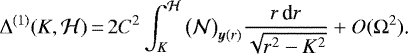
By inserting Eqs. (58) into (53) while considering (60), we obtain the integral form of the delay function up to the lth post-Minkowskian order
![Mathematical equation: \begin{align} \Delta^{(1)}(\bm{x}_A,\bm{x}_B)\;{=}&\;R_{AB}\int_{\mathcal D}\big(\mathcal N\big)_{\bm{z}(\sigma)}\textrm{d}\sigma\text{,}\\ \Delta^{(2)}(\bm{x}_A,\bm{x}_B)\;{=}&\;\frac{R_{AB}}{2}\nonumber\\ &\times\int_{\mathcal D}\Bigg\{\left(\mathcal N^2\right)_{\bm{z}(\sigma)}-\left[\frac{\partial\Delta^{(1)}}{\partial x^i}\frac{\partial\Delta^{(1)}}{\partial x^i}\right]_{(\bm{z}(\sigma),\bm{x}_B)}\Bigg\}\textrm{d}\sigma\text{,}\end{align}](/articles/aa/full_html/2021/04/aa40269-20/aa40269-20-eq113.png)
and, for l ≥ 3
![Mathematical equation: \begin{equation*} \Delta^{(l)}(\bm{x}_A,\bm{x}_B)\,{=}\,{-}\frac{R_{AB}}{2}\int_{\mathcal D}\ \sum_{m\,{=}\,1}^{l-1}\left[\frac{\partial\Delta^{(m)}}{\partial x^i}\frac{\partial\Delta^{(l-m)}}{\partial x^i}\right]_{(\bm{z}(\sigma),\bm{x}_B)}\textrm{d}\sigma\text{.}\end{equation*}](/articles/aa/full_html/2021/04/aa40269-20/aa40269-20-eq114.png) (61c)
(61c)
As mentioned previously by Bourgoin (2020), these equations show that the first-order delay is the well-known excess path delay due to the change of the phase velocity when the signal is crossing through  . The geometric delay shows up at the second post-Minkowskian order as well as the second-order correction to the excess path delay.
5.2 Stationary optical metric
Let us now assume that the fluid optical medium is at rest in a coordinate system rotating with respect to the global coordinate system. We use  to denote the rotating coordinate system1. The relationbetween the optical medium rest frame and the global coordinate system reads
 (62a)
(62a)
in which  are the elements of a rotation matrix. The inverse relation is given by
 (62b)
(62b)
with  being the elements of the inverse matrix. The relationships
 (63)
(63)
ensure that a transformation followed by its inverse is an identity transformation.
Differentiating Eqs. (62b) with respect to the global coordinate time returns the transformation law that relates the 3-velocities expressed in the two coordinate systems:
 (64)
(64)
Here, an overdot indicates differentiation with respect to t and ωâĉ is the angular velocity tensor being defined by
 (65)
(65)
The quantities  represent the components of the permutation symbol and ωâ is the âth component of the angular velocity vector expressed in the rotating coordinate system, namely
 (66)
(66)
where ω is the magnitude of the angular velocity of rotation and eâ is the âth component of the unit direction of the spin axis.
Hereafter, we assume that the time-dependent rotation matrix corresponds to a rigid uniform rotation so that the angular velocity tensor is constant, namely
 (67)
(67)
In addition, in the rotating frame, which is the rest frame of the medium, the 3-velocity vector of a particle of a fluid is null by definition, that is to say
 (68)
(68)
The expression for the velocity of a particle of a fluid expressed in the global coordinate system is derived after substituting ẋâ from Eqs. (68) into (64) which leads to
 (69)
(69)
Let ξ(x) be a coordinate 3-velocity vector field at the point-event x belonging to a fluid element of the optical medium. It is defined in global coordinate notation by
 (70)
(70)
Owing to Eqs. (65), (66), and (69), the coordinate 3-velocity vector of an element of the fluid dielectric medium is given in the global coordinate system by
 (71)
(71)
Thus, the unit 4-velocity vector of the medium reads
 (72)
(72)
The expression for the time component w0 is straightforwardly inferred from the fact that the 4-velocity is a unit vector for the physical metric of spacetime (see assumption (1)), hence w0 = Γ, where Γ is defined as
 (73)
(73)
We can now express the components of the optical metric from the relation in Eq. (6). The only non-null components are
![Mathematical equation: \begin{align} \kappa^{00}_{(1)}&\,{=}\,2\Gamma^2\mathcal N\text{,} \qquad \kappa^{0i}_{(1)}\,{=}\,\kappa^{00}_{(1)}\,\xi^i\text{,} \qquad \kappa^{ij}_{(1)}\,{=}\,\kappa^{00}_{(1)}\,\xi^i\xi^j\text{,}\\[5pt] \kappa^{00}_{(2)}&\,{=}\,\Gamma^2\mathcal N^2\text{,} \qquad \kappa^{0i}_{(2)}\,{=}\,\kappa^{00}_{(2)}\,\xi^i\text{,} \qquad \kappa^{ij}_{(2)}\,{=}\,\kappa^{00}_{(2)}\,\xi^i\xi^j\text{.}\end{align}](/articles/aa/full_html/2021/04/aa40269-20/aa40269-20-eq133.png)
As seen in Sect. 3, the index of refraction is defined in the instantaneous rest frame of the medium, namely the rotating frame. Thus, the index of refraction is independent of the time component of the rotating coordinate system, that is to say
![Mathematical equation: \begin{equation*} n(x^{\hat a})-1\,{=}\, \left\{ \begin{array}{l l} N_0\mathcal N(x^{\hat a}) & \mathrm{for}\ x^{\hat a}\in\mathcal{D}\text{,}\\[3pt] 0 & \mathrm{for}\ x^{\hat a}\notin\mathcal{D}\text{.} \end{array} \right. \end{equation*}](/articles/aa/full_html/2021/04/aa40269-20/aa40269-20-eq134.png) (75)
(75)
This statement implies that  according to the transformation rules in (62). Similarly, (71) also reveals that ∂0 ξi = 0, hence ∂0 Γ = 0. These simplifications imply that the optical metric is stationary, and so Eqs. (55) eventually reduce to
 (76)
(76)
By inserting (74) into (53) while considering (76), we obtain the integral form of the delay function up to the lth post-Minkowskian order:
![Mathematical equation: \begin{align} \Delta^{(1)}(\bm{x}_A,\bm{x}_B)\;{=}&\;R_{AB}\int_{\mathcal D}\left(\Gamma^2\mathcal N C^2\right)_{\bm{z}(\sigma)}\textrm{d}\sigma\text{,}\\[3pt] \Delta^{(2)}(\bm{x}_A,\bm{x}_B)\;{=}&\;\frac{R_{AB}}{2}\int_{\mathcal D}\Bigg\{\left(\Gamma^2\mathcal N^2C^2\right)_{\bm{z}(\sigma)}-\left[\frac{\partial\Delta^{(1)}}{\partial x^i}\frac{\partial\Delta^{(1)}}{\partial x^i}\right]_{(\bm{z}(\sigma),\bm{x}_B)}\nonumber\\[3pt] &+4\left(\Gamma^2\mathcal NC\xi^i\right)_{\bm{z}(\sigma)}\left[\frac{\partial\Delta^{(1)}}{\partial x^i}\right]_{(\bm{z}(\sigma),\bm{x}_B)}\Bigg\}\textrm{d}\sigma\text{,}\\[3pt] \Delta^{(3)}(\bm{x}_A,\bm{x}_B)\;{=}&\;R_{AB}\int_{\mathcal D}\Bigg\{\left(\Gamma^2\mathcal N\xi^i\xi^j\right)_{\bm{z}(\sigma)}\left[\frac{\partial\Delta^{(1)}}{\partial x^i}\frac{\partial\Delta^{(1)}}{\partial x^j}\right]_{(\bm{z}(\sigma),\bm{x}_B)}\nonumber\\[3pt] &+\left(\Gamma^2\mathcal N^2C\xi^i\right)_{\bm{z}(\sigma)}\left[\frac{\partial\Delta^{(1)}}{\partial x^i}\right]_{(\bm{z}(\sigma),\bm{x}_B)}\nonumber\\[3pt] &+2\left(\Gamma^2\mathcal NC\xi^i\right)_{\bm{z}(\sigma)}\left[\frac{\partial\Delta^{(2)}}{\partial x^i}\right]_{(\bm{z}(\sigma),\bm{x}_B)}\nonumber\\[3pt] &-\left[\frac{\partial\Delta^{(1)}}{\partial x^i}\frac{\partial\Delta^{(2)}}{\partial x^i}\right]_{(\bm{z}(\sigma),\bm{x}_B)}\Bigg\}\textrm{d}\sigma\text{,} \end{align}](/articles/aa/full_html/2021/04/aa40269-20/aa40269-20-eq137.png)
and, for l ≥ 4,
![Mathematical equation: \begin{align*} \Delta^{(l)}(\bm{x}_A,\bm{x}_B)\;{=}&\;\frac{R_{AB}}{2}\int_{\mathcal D}\Bigg\{-\sum_{m\,{=}\,1}^{l-1}\left[\frac{\partial\Delta^{(m)}}{\partial x^i}\frac{\partial\Delta^{(l-m)}}{\partial x^i}\right]_{(\bm{z}(\sigma),\bm{x}_B)}\nonumber\\[3pt] &+2\left(\Gamma^2\mathcal N\xi^i\xi^j\right)_{\bm{z}(\sigma)}\sum_{n\,{=}\,1}^{l-2}\left[\frac{\partial\Delta^{(n)}}{\partial x^i}\frac{\partial\Delta^{(l-n-1)}}{\partial x^j}\right]_{(\bm{z}(\sigma),\bm{x}_B)}\nonumber\\[3pt] &+\left(\Gamma^2\mathcal N^2\xi^i\xi^j\right)_{\bm{z}(\sigma)}\sum_{n\,{=}\,1}^{l-3}\left[\frac{\partial\Delta^{(n)}}{\partial x^i}\frac{\partial\Delta^{(l-n-2)}}{\partial x^j}\right]_{(\bm{z}(\sigma),\bm{x}_B)}\nonumber\\[3pt] &+4\left(\Gamma^2\mathcal NC\xi^i\right)_{\bm{z}(\sigma)}\left[\frac{\partial\Delta^{(l-1)}}{\partial x^i}\right]_{(\bm{z}(\sigma),\bm{x}_B)}\nonumber\\[3pt] &+2\left(\Gamma^2\mathcal N^2C\xi^i\right)_{\bm{z}(\sigma)}\left[\frac{\partial\Delta^{(l-2)}}{\partial x^i}\right]_{(\bm{z}(\sigma),\bm{x}_B)}\Bigg\}\textrm{d}\sigma\text{.} \end{align*}](/articles/aa/full_html/2021/04/aa40269-20/aa40269-20-eq138.png) (77d)
(77d)
We introduced C and D as
 (78)
(78)
Hereafter, C is referred to as the geometric factor and D as the light-dragging term.
By comparing Eqs. (77a) and (61a), it is seen that the dynamics of the optical medium affects the expression of the delay function as soon as the first post-Minkowskian order. Hereafter, we solve Eqs. (77a) assuming a spherically symmetric optical metric.
5.3 Spherical symmetry
Let us assume that the optical medium is the planetary neutral atmosphere of the occulting body. The global coordinate system is supposed to be centered at the center of mass of the occulting body and is nonrotating with respect to distant stars. The medium is assumed to be at rest in the frame rotating with the planet (i.e., the medium rest frame). The atmosphere of the occulting body is assumed to be spherically symmetric so centrifugal effects due to the rotation are neglected. In that respect,  draws a timelike tube defining the spacetime boundaries of the planetary neutral atmosphere (see Fig. 1).
The spherical symmetry assumption allows us to determine the limits of integration in Eq. (77). Let  be the radius of the top neutral atmosphere. The intersection between the path of integration and
  can be determined from Eq. (41) as
 (79)
(79)
After a little algebra, we find
 (80)
(80)
where we have introduced
 (81)
(81)
This latter expression suggests that K is the impact parameter with respect to the center of symmetry (i.e., the center of mass of the occulting planet).
Let xK be the point-event defined by xK ≡ z(σK). After substituting σK from Eqs. (80) into (54), we find the spacetime components of  with
with

It can be seen that K = ∥xK∥, and therefore the unit 3-vector for the direction of xK, namely nK = xK∕K, is given by
 (83)
(83)
Therefore, xK is the point-event along the path of integration where the euclidean distance with respect to the center of symmetry is the smallest. Let us note that Eq. (83) implies that
 (84)
(84)
Accordingly,it is helpful to introduce the unit 3-vector SAB such that the triad of vectors (nK, NAB, SAB) forms a right-handed vector basis. That is to say
 (85)
(85)
After identifying Eq. (85) with (83), we deduce
 (86)
(86)
The unit vector SAB is therefore recognized to be the direction of the angular momentum vector of the zeroth-order null geodesic path (Teyssandier 2012).
Let x+ and x− be the point-events defined by x±≡ z(σ±). After substituting σ± from Eq. (80) into (54), we find the spacetime components of  with
with

The point-event x+ is the spacetime point where the zeroth-order null geodesic path is entering  , and conversely, x− is the spacetime point where the zeroth-order null geodesic path is exiting
  as shown in Fig. 1.
Therefore, in the context of radio occultations by a spherically symmetric atmosphere, any integral over the refractive domain, such as
 (88)
(88)
where f is a known function which varies over the path of integration, can now be written as
![Mathematical equation: \begin{equation*} I(\bm{x}_A,\bm{x}_B)\,{=}\,\frac{R_{AB}}{2}\left[\int_{\sigma_-}^{\sigma_K}f\big(\bm{z}(\sigma)\big)\,\textrm{d}\sigma+\int_{\sigma_K}^{\sigma_+}f\big(\bm{z}(\sigma)\big)\,\textrm{d}\sigma\right]\text{.}\end{equation*}](/articles/aa/full_html/2021/04/aa40269-20/aa40269-20-eq157.png) (89)
(89)
By separating the path of integration as

where χ is a new variable with
 (90c)
(90c)
and making use of Eqs. (82b), (87b), and Eq. (41), we find that (89) can also be written as
![Mathematical equation: \begin{align*} I(\bm{x}_A,\bm{x}_B)\;{=}&\;\frac{\sqrt{\mathcal H^2-K^2}}{2}\nonumber\\ &\times\left[\int_{0}^{1}f\big(\bm{y}_-(\chi)\big)\,\textrm{d}\chi+\int_{0}^{1}f\big(\bm{y}_+(\chi)\big)\,\textrm{d}\chi\right]\text{.}\end{align*}](/articles/aa/full_html/2021/04/aa40269-20/aa40269-20-eq160.png) (91)
(91)
The spherical symmetry implies that f = f(r), and so it is more convenient to integrate toward the radial component r. To perform the change of variable, we can introduce r as follows
 (92)
(92)
and resolve for χ considering condition Eq. (90c), that is to say
 (93)
(93)
The expressions for the differentials of χ± are given by
 (94)
(94)
such that Eq. (91) now reads
 (95a)
(95a)
where the path of integration satisfies ∥y(r)∥ = r and is given by
 (95b)
(95b)
Because the relations in Eq. (77) are the same as those in Eq. (88), which is itself equivalent to Eq. (95a), the 3-velocity of the medium must be evaluated along y(r) within the assumption of spherical symmetry. From Eqs. (95b) and (71), we infer
 (96)
(96)
where we introduce
 (97)
(97)
We can immediately see from Eqs. (84), (85), and (96) that the scalar product of the dragging term in Eq. (78) is actually independent of r and can therefore be considered constant during integration along y(r). Thus, the light-dragging coefficient reads
 (98)
(98)
According to Eq. (78), we deduce that the geometric factor C is independent of r too.
6 Mathematical modeling
According to relations (77), we now need a mathematical expression describing the radial evolution of refractivity in order to derive the expressions for the time and frequency transfers.
We emphasize that the method usually employed for processing radio occultation data proceeds the other way around. Indeed, the refractivity profile is usually determined from the frequency transfer by employing Abel inversion (Phinney & Anderson 1968) or numerical ray-tracing (Schinder et al. 2015) methods. Here, the approach is more closely related to a model-fitting parameter method. Indeed, we first build a mathematical modeling for the refractivity profile and then we deduce the consequences at the level of the observables, namely the time and frequency transfers. In principle, the last step should be to compare these computed observables to real ones in order to minimize the differences by estimating the parameters of the model (i.e., the parameters entering the refractivity profile) using for instance a standard least-squares fit.
In Appendix A, we comment on how the ideas of Sect. 5 can indeed be applied in the context of an Abel inversion method while accounting for the light-dragging effect, such that no a priori modeling for the refractive profile is required.
6.1 Refractivity profile
In the context of atmospheric occultation experiments, a priori knowledge of the atmospheric composition must be assumed. In what follows, the refractive medium is assumed to be an ideal gas. Taking h to denote the altitude above ground level, that is
 (99)
(99)
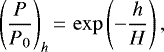
where R is the value of the radial coordinate for the points such that N = N0, the pressure profile is given by
 (100)
(100)
where Nv is the refractive volume (Fjeldbo & Eshleman 1968), T the temperature, and k the Boltzmann constant:
 (101)
(101)
From Eq. (100), we deduce the following expression:
 (102)
(102)
where P0 and T0 are the pressure and temperature at ground level, respectively. The refractivity at ground level N0 is
 (103)
(103)
The refractivity profile in Eq. (102) is eventually proportional to the product of two functions, namely  and
and  . However, let us emphasize that for planetary atmospheres the temperature usually varies much more slowly than the pressure across the profile. Therefore, in some application that does not necessitate high precision, it might be convenient to consider that
  is constant (isotherm atmosphere) with respect to
  . In this work, we do not make such a simplification and we consider that the temperature is a function of the altitude inside the atmosphere.
Planetary neutral atmospheres all admit an exponential pressure profile as a first approximation (Withers 2010), meaning that it is common to model the pressure as
 (104)
(104)
where H is a constant parameter called the scale height of the neutral atmosphere and has length dimension (L). The large-scale temperature variation across the atmospheric profile can then be expressed as a polynomial function of degree d, namely
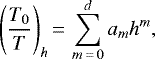 (105)
(105)
where am are the polynomial coefficients and have dimension L−m. Because T0 is the temperature at ground level (i.e., h = 0 km), it follows that
 (106)
(106)
The series expansion in Eq. (105) is easily changed into a function of r with Eq. (99). After a little algebra, we find
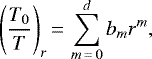 (107)
(107)
where the bm coefficients have dimension L−m and are given by
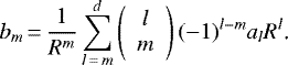 (108)
(108)
The binomial coefficient is defined as
 (109)
(109)
In the context of radio occultation experiments, it is more convenient to express the profiles in terms of η the altitude above the impact parameter, namely
 (110)
(110)
The advantage for using η instead of r relies on the fact that most applications satisfy η ≪ K everywhere in  which allows us to look for solutions in an infinite series in ascending power of η∕K. Accordingly,the temperature variation now reads
 (111)
(111)
with
 (112a)
or, after substituting bl from (108),
 (112b)
Once expressed in terms of η, the pressure profile now reads
 (113)
(113)
where PK is the pressureat the level of the impact parameter and is given by Eq. (104), that is to say
 (114)
(114)
The expression for  can be inferred after inserting Eqs. (113) and (111) into (102). Finally, by invoking the definition (50), we eventually find
 (115)
(115)
Let us evaluate this last relationship at the top of the atmosphere and for the optical ray grazing event, namely  with
with  . A simple substitution into Eq. (115) returns
 (116)
(116)
This result shows that refractivity is non-null on the limits of the refractive domain  . In order to ensure a smooth transition between the inside of the domain
  (where the refractivity should be N≠0) and the outside (where the refractivity should be N = 0), we would rather introduce
  such as
 (117)
(117)
In the context of radio occultation experiments, the value of  should be adjusted such that the effect of
  becomes unobservable, that is to say
  . As seen from Eq. (116), this can be achieved by taking the limit
  . Hereafter, we continue the discussion keeping
  at an arbitrary value for completeness.
In practice, parameters H and bm (or am) would now need to be determined by confrontation with observations. To do so, we need to derive the expressions for the time and the frequency transfers resulting from Eq. (117).
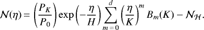
6.2 The time transfer function
A direct integration of relations (77) is difficult in the context of a purely post-Minkowskian expansion in ascending power of N0. The main difficulty is related to the arbitrariness in the magnitude of the velocity of the medium. However, everywhere within the Solar System, we are only dealing with planetary atmospheres with Ω ≪ 1. Consequently, Γ2 in Eq. (73), that is,
![Mathematical equation: \begin{equation*} \Gamma^2(r)\,{=}\,\Big[1-\bm{\xi}\big(\bm{y}(r)\big)\cdot\bm{\xi}\big(\bm{y}(r)\big)\Big]^{-1}\text{,}\end{equation*}](/articles/aa/full_html/2021/04/aa40269-20/aa40269-20-eq205.png) (118)
(118)
can be expanded as
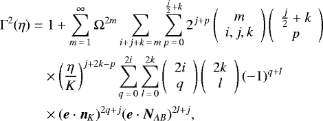 (119)
(119)
where the multinomial coefficient is defined by
 (120)
(120)
This expansion shows that the first nonconstant contribution in Γ2 is a second-order term in Ω.
Hereafter, in order to simplify computations, we consider terms up to first order in Ω, so that we now assume
 (121)
(121)
Therefore, the geometric factor (introduced in Eq. (78)) is the only term that is contributing at first order in Ω:
 (122)
(122)
By making use of Eqs. (88) and (95a), we see that (77a) can be written as follows
 (123)
(123)
Then, by invoking Eq. (110), the function to be integrated can be written as an expansion in ascending power of η∕K, that is to say
 (124)
(124)
where Qm is given by
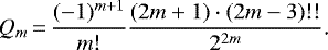 (125)
(125)
The double factorial (Arfken 1985) is defined by
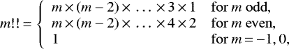 (126a)
and by
 (126b)
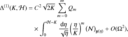
After substituting  from Eqs. (117) into (124), we arrive at the following expression:
![Mathematical equation: \begin{align*} \Delta^{(1)}(K,\mathcal H)\;{=}&\;C^2\,\Bigg[\sum_{m\,{=}\,0}^{\infty}\mathcal{L}_m(K,\mathcal{H})\sum_{n\,{=}\,0}^{m_d}Q_{m-n}B_n(K)\nonumber\\ &-B_0(\mathcal H)\sum_{m\,{=}\,0}^{\infty}Q_m\mathcal{M}_m(K,\mathcal{H})\Bigg]+O(\Omega^{2})\text{,}\end{align*}](/articles/aa/full_html/2021/04/aa40269-20/aa40269-20-eq216.png) (127)
(127)
with

and
 (129)
(129)
Each  and
and  can now be integrated exactly. The solutions for the first terms (i.e., m = 0) are given by
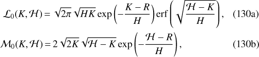
where erf(x) denotes the well-known error function
 (131)
(131)
The following solutions (i.e., m ≥ 1) are convenientlyexpressed in terms of  ,
,  , and the mth power of H∕K:
![Mathematical equation: \begin{align} \mathcal{L}_m(K,\mathcal{H})\;{=}&\;\frac{(2m-1)!!}{2^m}\left(\frac{H}{K}\right)^m\nonumber\\ &\times\left[\mathcal{L}_0-\mathcal{M}_0\sum_{p\,{=}\,0}^{m-1}\frac{2^p}{(2p+1)!!}\left(\frac{\mathcal{H}-K}{H}\right)^p\right]\text{,}\\ \mathcal{M}_m(K,\mathcal{H})\;{=}&\;\frac{\mathcal{M}_0}{(2m+1)}\left(\frac{H}{K}\right)^m\left(\frac{\mathcal H-K}{H}\right)^m\text{.}\end{align}](/articles/aa/full_html/2021/04/aa40269-20/aa40269-20-eq225.png)
It is seen from Eq. (130) that both  and
and  vanish when
  . In addition, both
  and
and  are only defined for
  . Indeed,
  would return a nonphysical imaginary number. This fact states that the refractive delay due to the optical medium is only observed for an optical ray crossing through the refractive domain
  as expected.
Finally, the expression for the first-order delay function is inferred after substituting  and
and  from Eqs. (132) into (127) which eventually returns
 (133)
(133)
where
 (134a)
![Mathematical equation: \begin{align*} \Delta^{(1)}_{\mathcal M_0}(K,\mathcal H)\;{=}&\;-\mathcal{M}_0\Bigg[\sum_{m\,{=}\,1}^{\infty}\frac{(2m-1)!!}{2^m}\left(\frac{H}{K}\right)^m\nonumber\\ &\times\sum_{p\,{=}\,0}^{m-1}\frac{2^p}{(2p+1)!!}\left(\frac{\mathcal{H}-K}{H}\right)^p\sum_{n\,{=}\,0}^{m_d}Q_{m-n}B_n(K)\nonumber\\ &+B_0(\mathcal H)\sum_{m\,{=}\,0}^{\infty}\frac{Q_m}{(2m+1)}\left(\frac{H}{K}\right)^m\left(\frac{\mathcal H-K}{H}\right)^m\Bigg]\text{.}\end{align*}](/articles/aa/full_html/2021/04/aa40269-20/aa40269-20-eq238.png) (134b)
(134b)
After substituting K, C2, and SAB from Eqs. (81), (122), and (86), respectively, into Eqs. (130), (133), and (134), we find the expression for the delay function in terms of xA and xB, as is usually done in the literature for time transfer functions. We eventually get a relationship as follows
 (135)
(135)
We recall that the global frame is centered at the occulting body center of mass and is nonrotating with respect to distant stars. The atmosphere is still in the frame attached to the occulting body, namely the rotatingframe. The refractivity profile is given by Eq. (102), where the pressure profile is an exponential function and where the temperature profile is a polynomial function of arbitrary degree d.
6.3 Frequency transfer
Hereafter, we focus on the determination of the frequency transfer. After inserting Eqs. (36) and (52) into (33), we deduce
 (136)
(136)
where the components of the covectors  and
and  have been introduced such as

with
![Mathematical equation: \begin{align*} \underline{\bm{l}}_A^{(m)}(\bm{x}_A,\bm{x}_B)&\,{=}\,\left[\frac{\partial\Delta^{(m)}}{\partial\bm{x}_A}\right]_{(\bm{x}_A,\bm{x}_B)}\text{,}\\ \underline{\bm{l}}_B^{(m)}(\bm{x}_A,\bm{x}_B)&\,{=}\,-\left[\frac{\partial\Delta^{(m)}}{\partial\bm{x}_B}\right]_{(\bm{x}_A,\bm{x}_B)}\text{.} \end{align*}](/articles/aa/full_html/2021/04/aa40269-20/aa40269-20-eq244.png)
In order to derive the explicit expression for the frequency transfer, we need to determine  and
and  . To do so we have to find the derivative of the time delay with respect to the impact parameter, and then the derivative of K with respect to the components of the position vectors at the level of the emission and reception. The latter derivatives are easily inferred from Eq. (81) and after inserting them into Eq. (138), we end up with
![Mathematical equation: \begin{align} \underline{\bm{l}}_A^{(m)}(\bm{x}_A,\bm{x}_B)&\,{=}\,\bm{n}_K\left(\frac{\bm{N}_{AB}\cdot\bm{x}_B}{R_{AB}}\right)\left[\frac{\partial\Delta^{(m)}}{\partial K}\right]_{(\bm{x}_A,\bm{x}_B)}\text{,}\\ \underline{\bm{l}}_B^{(m)}(\bm{x}_A,\bm{x}_B)&\,{=}\,{-}\bm{n}_K\left(1-\frac{\bm{N}_{AB}\cdot\bm{x}_B}{R_{AB}}\right)\left[\frac{\partial\Delta^{(m)}}{\partial K}\right]_{(\bm{x}_A,\bm{x}_B)}\text{.}\end{align}](/articles/aa/full_html/2021/04/aa40269-20/aa40269-20-eq247.png)
Equations Eqs. (139) together with (83) and (84) show that the directions  and
and  are unit triplets at the first post-Minkowskian order (i.e., m = 1), namely
 (140)
(140)
In addition, we notice from Eq. (139b) that the covector at reception can be written such as
![Mathematical equation: \begin{equation*} \underline{\bm{l}}_B\,{=}\,\underline{\bm{l}}_A-\bm{n}_K\sum_{m\,{=}\,1}^{\infty}(N_0)^m\left[\frac{\partial\Delta^{(m)}}{\partial K}\right]_{(\bm{x}_A,\bm{x}_B)}\text{,} \end{equation*}](/articles/aa/full_html/2021/04/aa40269-20/aa40269-20-eq251.png) (141)
(141)
which shows, after invoking (85), that
![Mathematical equation: \begin{equation*} \underline{\bm{l}}_A\,{\times}\,\underline{\bm{l}}_B\,{=}\,{-}\bm{S}_{AB}\sum_{m\,{=}\,1}^{\infty}(N_0)^m\left[\frac{\partial\Delta^{(m)}}{\partial K}\right]_{(\bm{x}_A,\bm{x}_B)}\text{,} \end{equation*}](/articles/aa/full_html/2021/04/aa40269-20/aa40269-20-eq252.png) (142)
(142)
These relations are useful for defining the bending angle ϕ. Usually, this angle is introduced using the scalar product between the two tangent vectors; however in order to avoid numerical errors, especially when dealing with small angles, it is more appropriate to introduce ϕ such as
![Mathematical equation: \begin{equation*} \phi(\bm{x}_A,\bm{x}_B)\,{=}\,\arcsin\left[\frac{\underline{\bm{l}}_A\,{\times}\,\underline{\bm{l}}_B}{\Vert\underline{\bm{l}}_A\Vert\,\Vert\underline{\bm{l}}_B\Vert}\cdot\bm{S}_{AB}\right]\text{.} \end{equation*}](/articles/aa/full_html/2021/04/aa40269-20/aa40269-20-eq253.png) (143)
(143)
Therefore, it is seen from Eqs. (137) that the bending angle assumes a post-Minkowskian expansion too, namely
 (144)
(144)
where the first-order term satisfies
![Mathematical equation: \begin{equation*} \phi^{(1)}(\bm{x}_A,\bm{x}_B)\,{=}\,-\Bigg[\frac{\partial\Delta^{(1)}}{\partial K}\Bigg]_{(\bm{x}_A,\bm{x}_B)}\text{.}\end{equation*}](/articles/aa/full_html/2021/04/aa40269-20/aa40269-20-eq255.png) (145)
(145)
The last missing piece is now the derivative of the time delay with respect to the impact parameter K. This latter can be derived from Eqs. (133) and (134) as
![Mathematical equation: \begin{align*} \Bigg[\frac{\partial \Delta^{(1)}}{\partial K}\Bigg]_{(K,\mathcal H)}\;{=}&\;C^2\left(\frac{\partial \Delta^{(1)}_{\mathcal L_0}}{\partial K}+\frac{\partial \Delta^{(1)}_{\mathcal M_0}}{\partial K}\right)_{(K,\mathcal H)}\nonumber\\ &{-}\frac{2D}{K}\left(\Delta^{(1)}_{\mathcal L_0}+\Delta^{(1)}_{\mathcal M_0}\right)_{(K,\mathcal H)}+O(\Omega^2)\text{,}\end{align*}](/articles/aa/full_html/2021/04/aa40269-20/aa40269-20-eq256.png) (146)
(146)
where
![Mathematical equation: \begin{align*} \Bigg[\frac{\partial \Delta^{(1)}_{\mathcal L_0}}{\partial K}\Bigg]_{(K,\mathcal H)}\;{=}&\;{-}\frac{\mathcal L_0}{H}\sum_{m\,{=}\,0}^{\infty}\frac{(2m-1)!!}{2^m}\left(\frac{H}{K}\right)^m\nonumber\\ &\times\sum_{n\,{=}\,0}^{m_d}Q_{m-n}\sum_{l\,{=}\,n}^{d}\left( \begin{array}{c} l\\ n \end{array} \right)b_lK^{l}\nonumber\\ &\times\left[1+\left(\frac{H}{K}\right)\left(m-l-\frac{1}{2}+\frac{\mathcal{M}_0}{2\mathcal{L}_0}\frac{K}{\mathcal H-K}\right)\right]\text{,} \end{align*}](/articles/aa/full_html/2021/04/aa40269-20/aa40269-20-eq257.png) (147a)
(147a)
![Mathematical equation: \begin{align*} \Bigg[\frac{\partial \Delta^{(1)}_{\mathcal M_0}}{\partial K}\Bigg]_{(K,\mathcal H)}\;{=}&\;\frac{\mathcal M_0}{K}\Bigg\{\sum_{m\,{=}\,1}^{\infty}\frac{(2m-1)!!}{2^m}\left(\frac{H}{K}\right)^m\sum_{n\,{=}\,0}^{m_d}Q_{m-n}\nonumber\\ &\times\sum_{l\,{=}\,n}^{d}\left( \begin{array}{c} l\\ n \end{array} \right)b_lK^{l}\sum_{p\,{=}\,0}^{m-1}\frac{2^p}{(2p+1)!!}\left(\frac{\mathcal H-K}{H}\right)^p\nonumber\\ &\times\left[\frac{2(p-m+l+1)K+(2m-2l-1)\mathcal H}{2(\mathcal H-K)}\right]\nonumber\\ &+B_0(\mathcal H)\sum_{m\,{=}\,0}^{\infty}\frac{Q_m}{(2m+1)}\left(\frac{H}{K}\right)^m\left(\frac{\mathcal H-K}{H}\right)^m\nonumber\\ &\times\left[\frac{2K+(2m-1)\mathcal H}{2(\mathcal H-K)}\right]\Bigg\}\text{.} \end{align*}](/articles/aa/full_html/2021/04/aa40269-20/aa40269-20-eq258.png) (147b)
(147b)
After substituting K, C2, D, and SAB from Eqs. (81), (122), (98), and (86), respectively, into Eqs. (146) and (147), we find expressions for the derivatives in terms of xA and xB, as is usually done in the literature for time transfer functions. The expressions for  and
and  are obtained after inserting Eqs. (146) and () into (139) and (137), and then the frequency transfer is simply given by Eqs. (136) and (32).
6.4 Limits when the atmosphere radius 
As mentioned in Sect. 6.1, in the context of radio occultation experiments, the effect of refractivity is often negligible when the impact parameter K approaches  . This is mainly due to the fast decrease of the exponential pressure profile when the value of the impact parameter increases.
We see above that the refractive profile in Eq. (117) has the expected limit when  . Hence, if one is interested in applications for occultation experiments, one can safely replace
  and
and  (in Eqs. (130)) by their following limits:

meaning that all terms proportional to  vanish.
Therefore, the time transfer function simplifies to
![Mathematical equation: \begin{align*} \mathcal{T}(\bm{x}_A,\bm{x}_B)\;{=}&\;\frac{\Vert\bm{x}_B-\bm{x}_A\Vert}{c}\nonumber\\ &+\frac{N_0}{c}\left[1+2\bm{\Omega}\cdot\frac{\bm{N}_{AB}\times\bm{x}_B}{\Vert\bm{N}_{AB}\times\bm{x}_B\Vert}+O(\Omega^{2})\right]\nonumber\\ &\times\sqrt{2\pi}\sqrt{H}\sqrt{\Vert\bm{N}_{AB}\times\bm{x}_B\Vert}\exp\left(-\frac{\Vert\bm{N}_{AB}\,{\times}\,\bm{x}_B\Vert-R}{H}\right)\nonumber\\ &\times\sum_{m\,{=}\,0}^{\infty}\frac{(2m-1)!!}{2^m}\left(\frac{H}{\Vert\bm{N}_{AB}\,{\times}\,\bm{x}_B\Vert}\right)^{m}\nonumber\\ &\times\sum_{n\,{=}\,0}^{m_d}Q_{m-n}\sum_{l\,{=}\,n}^{d}\left( \begin{array}{c} l\\ n \end{array}\right)b_l\Vert\bm{N}_{AB}\,{\times}\,\bm{x}_B\Vert^l+O(N_0^2)\text{.}\end{align*}](/articles/aa/full_html/2021/04/aa40269-20/aa40269-20-eq268.png) (149)
(149)
Similarly, the covectors  and
and  are now given by
![Mathematical equation: \begin{align*} \underline{\bm{l}}_A(\bm{x}_A,\bm{x}_B)\;{=}&\;{-}\bm{N}_{AB}\nonumber\\ &-N_0\sqrt{2\pi}\sqrt{\frac{\Vert\bm{N}_{AB}\,{\times}\,\bm{x}_B\Vert}{H}}\left(\frac{\bm{N}_{AB}\cdot\bm{x}_B}{R_{AB}}\right)\nonumber\\ &\times\exp\left(-\frac{\Vert\bm{N}_{AB}\,{\times}\,\bm{x}_B\Vert-R}{H}\right)\nonumber\\ &\times\sum_{m\,{=}\,0}^{\infty}\frac{(2m-1)!!}{2^m}\left(\frac{H}{\Vert\bm{N}_{AB}\,{\times}\,\bm{x}_B\Vert}\right)^m\nonumber\\ &\times\sum_{n\,{=}\,0}^{m_d}Q_{m-n}\sum_{l\,{=}\,n}^{d}\left( \begin{array}{c} l\\ n \end{array} \right)b_l\Vert\bm{N}_{AB}\,{\times}\,\bm{x}_B\Vert^{l}\nonumber\\ &\times\Bigg\{1+\frac{H}{\Vert\bm{N}_{AB}\,{\times}\,\bm{x}_B\Vert}\left(m-l-\frac{1}{2}\right)+2\bm{\Omega}\cdot\frac{\bm{N}_{AB}\,{\times}\,\bm{x}_B}{\Vert\bm{N}_{AB}\,{\times}\,\bm{x}_B\Vert}\nonumber\\ &\times\left[1+\frac{H}{\Vert\bm{N}_{AB}\,{\times}\,\bm{x}_B\Vert}\left(m-l-\frac{3}{2}\right)\right]+O(\Omega^2)\Bigg\}\nonumber\\ &\times\Bigg.\frac{\bm{N}_{AB}\,{\times}\,\bm{x}_B}{\Vert\bm{N}_{AB}\,{\times}\,\bm{x}_B\Vert}\,{\times}\,\bm{N}_{AB}+O(N_0^2)\text{,} \end{align*}](/articles/aa/full_html/2021/04/aa40269-20/aa40269-20-eq271.png) (150a)
(150a)
and
![Mathematical equation: \begin{align*} \underline{\bm{l}}_B(\bm{x}_A,\bm{x}_B)\;{=}&\;{-}\bm{N}_{AB}\nonumber\\ &+N_0\sqrt{2\pi}\sqrt{\frac{\Vert\bm{N}_{AB}\,{\times}\,\bm{x}_B\Vert}{H}}\left(1-\frac{\bm{N}_{AB}\cdot\bm{x}_B}{R_{AB}}\right)\nonumber\\ &\times\exp\left(-\frac{\Vert\bm{N}_{AB}\,{\times}\,\bm{x}_B\Vert-R}{H}\right)\nonumber\\ &\times\sum_{m\,{=}\,0}^{\infty}\frac{(2m-1)!!}{2^m}\left(\frac{H}{\Vert\bm{N}_{AB}\,{\times}\,\bm{x}_B\Vert}\right)^m\nonumber\\ &\times\sum_{n\,{=}\,0}^{m_d}Q_{m-n}\sum_{l\,{=}\,n}^{d}\left( \begin{array}{c} l\\ n \end{array} \right)b_l\Vert\bm{N}_{AB}\,{\times}\,\bm{x}_B\Vert^{l}\nonumber\\ &\times\Bigg\{1+\frac{H}{\Vert\bm{N}_{AB}\,{\times}\,\bm{x}_B\Vert}\left(m-l-\frac{1}{2}\right)+2\bm{\Omega}\cdot\frac{\bm{N}_{AB}\,{\times}\,\bm{x}_B}{\Vert\bm{N}_{AB}\,{\times}\,\bm{x}_B\Vert}\nonumber\\ &\times\left[1+\frac{H}{\Vert\bm{N}_{AB}\,{\times}\,\bm{x}_B\Vert}\left(m-l-\frac{3}{2}\right)\right]+O(\Omega^2)\Bigg\}\nonumber\\ &\times\Bigg.\frac{\bm{N}_{AB}\,{\times}\,\bm{x}_B}{\Vert\bm{N}_{AB}\,{\times}\,\bm{x}_B\Vert}\,{\times}\,\bm{N}_{AB}+O(N_0^2)\text{.} \end{align*}](/articles/aa/full_html/2021/04/aa40269-20/aa40269-20-eq272.png) (150b)
(150b)
The expression for the frequency transfer is directly inferred after inserting these last two expressions into (136) while making use of (32).
7 Numerical ray-tracing
In this section, we perform a numerical integration of the equations for optical rays toward a spherically symmetric, rigidly rotating planetary atmosphere. We consider the case of an atmosphere with drastic changes in its temperature profile. We simulate thetime and frequency transfers for a one-way downlink between an emitter in Keplerian orbit around the occulting planet and a receiver at infinity. We compare the numerical results to analytical solutions derived in Sect. 6.
7.1 Optical rays equations
The equations for optical rays propagating in a nondispersive isotropic medium are derived in Sect. 3 (see Eqs. (19)). However, they can be further simplified. Indeed, above we assume that the optical metric is spherically symmetric, constant, and stationary. Accordingly, the time component of the 4-wave vector is a first integral because it remains constant during the propagation of the radio signal through  . In addition, we assume that the velocity of the medium is small with respect to the speed of light in a vacuum so we may only consider terms up to first order in ω∕c. With these simplifications, the equations for optical rays eventually read as follows
![Mathematical equation: \begin{align*} &\frac{\textrm{d} x^0}{\textrm{d}\ell}\,{=}\,n\text{,}\\ &\frac{\textrm{d}\bm{x}}{\textrm{d}\ell}\,{=}\,\frac{1}{n}\left[-\underline{\bm{l}}+\frac{\omega}{c}(n^2-1)\bm{e}\,{\times}\,\bm{x}\right]\text{,}\\ &\frac{\textrm{d}\underline{\bm{l}}}{\textrm{d}\ell}\,{=}\,{-}\bm{\nabla} n+\frac{\omega}{c}\frac{(n^2-1)}{n}\bm{e}\,{\times}\,\underline{\bm{l}}\text{.} \end{align*}](/articles/aa/full_html/2021/04/aa40269-20/aa40269-20-eq274.png)
We emphasize that these equations reduce to the classical set of equations of geometrical optics when ω∕c → 0 (see Sect. 3.2.1 of Born & Wolf 1999 and also Sect. 85 of Landau & Lifshitz 1960).
Let us assume that the global frame (eX, eY, eZ) is centered at the planet’s center of mass and is nonrotating with respect to distant stars. The (eX, eY) plane is chosen to coincide with the equator of the occulting planet. The eZ axis is aligned with the planet instantaneous axis of rotation, that is to say eZ = e. For convenience, we consider the case of an emitter at infinity whose direction vector is lying in the equatorial plane, so that we can choose to define eY = −NAB. The orbit of the emitter is characterized by the usual set of Keplerian elements, namely (aA, eA, ιA, ΩA, ωA, τA). Values of the selected Keplerian elements are given in Table 1. The Cartesian position and velocity of the emitter in the global frameare then given by Eqs. (3.40) and (3.41) of Poisson & Will (2014). By substituting the Keplerian elements from Table 1 into Eq. (3.44) of Poisson & Will (2014), it is seen that the direction of the pericenter coincides with eY -axis.
We consider that the mass and radius of the occulting planet are similar to those of Titan, that is to say M = 1.35 × 10²³ kg and R = 2 574 km. However, in order to truly assess the accuracy of analytical solutions, we consider more extreme atmospheric physical properties than those of the Titan atmospheric model of Waite et al. (2012). For instance, we would rather consider a completely fictional temperature profile exhibiting high vertical gradients as shown in Fig. 2 (see plain curve). In addition, we assume that the atmosphere is rapidly rotating with an angular rate of 2π rad s−1, so that the relativistic light-dragging term at the surface reaches Ω = 0.05.
The equations for optical rays are numerically integrated considering the following spherically symmetric index of refraction profile inside the domain  (see discussion in Sect. 6.1)
 (152a)
with r = ∥x∥ and
 (152b)
The values of polynomial coefficients bm are given in Table 2 for d = 6. The size of the domain  is taken to be
  , corresponding to an atmosphere thickness of 600 km. We consider a scale height of H = 20 km (similar to that of Titan), and use values of N0 (post-Minkowskian parameter of the theory) ranging from 10−3 to 10−6 for illustrative purposes.
The equations for optical rays are only integrated inside the refractive domain  . Outside, optical rays are simply assumed to propagate along straight lines according to the assumption (1).
Values of Keplerian elements of the emitter.
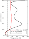 |
Fig. 2 Temperature profiles inside the atmosphere of the occulting planet. The plain curve represents a sixth-degree polynomial temperature profile, the dashed line represents an isothermal atmospheric profile, and the dotted line is the Titan atmospheric model of Waite et al. (2012). |
Values of bm coefficients for the determination of a sixth-degree polynomial temperature profile.
7.2 Numerical integration and initial pointing
The initial pointing direction at the level of the emitter is first assumed to be
 (153)
(153)
The spacetime coordinates of the ray entrance point-event inside the atmosphere can always be determined once the initial pointing direction is known. Let (ctE, xE) be the coordinates of the entrancepoint-event xE. It is clear that both tE and xE are functions of  , that is to say
  and
and  .
.
The initial pointing direction in Eq. (153) implies that xE ≡ x+ (see Eqs. (87)) for the first iteration. Then, having the coordinates of xE, the equations for optical rays in Eq. (151) can now be numerically integrated starting with ℓE = c(tE − tA) (we have defined tA as the origin of the coordinate time for the numerical integration) and

The numerical integration is stopped when the optical ray crosses the refractive domain  on the opposite side with respect to the entrance point-event xE. Let (ctF, xF) be the coordinates of xF, the final point-event for the numerical integration, that is to say

It is clear that the coordinates of xF depend on the initial conditions that have been used for conducting the numerical integration, namely  .
.
In general, because refractivity in  causes the optical ray to depart from its original direction, the direction of the ray at the exit of the atmosphere does not match the direction of the receiver. In order to make the two directions coincide, the initial pointing is iteratively corrected using a Newton-Raphson method (Press et al. 1992) for finding
  from the following condition
 (156)
(156)
Equations (151) are numerically integrated between Eqs. (154) and (155) assuming a relative numerical error tolerance of 10−12. The components of  are iteratively determined from (156) with the exact same accuracy. The partial derivatives of
  with respect to
  , which are needed for solving the initial pointing from Eq. (156), are determined using a second-order finite difference method. Finally, the time and frequency transfers are computed from numerical solutions of tF, xF, and
  .
.
The well-known atmospheric delay is given by the difference between the total light-time needed for reaching xF from xA and the projection of xF −xA along NAB, namely
 (157)
(157)
The expression for the relative Doppler frequency shift due to the atmosphere, and for the case of an observer at infinity, is obtained after inserting  into (32) and (136), which eventually returns
![Mathematical equation: \begin{equation*} \frac{\Delta\nu_B}{[\nu_B]_{\mathrm{vac}}}\,{=}\,\frac{\nu_B-[\nu_B]_{\mathrm{vac}}}{[\nu_B]_{\mathrm{vac}}}\,{=}\,{-}\frac{\bm{\beta}_A\cdot(\underline{\bm{l}}_A+\bm{N}_{AB})}{1+\bm{\beta}_A\cdot\underline{\bm{l}}_A}\text{,}\end{equation*}](/articles/aa/full_html/2021/04/aa40269-20/aa40269-20-eq298.png) (158)
(158)
where ![Mathematical equation: $[\nu_B]_{\mathrm{vac}}$](/articles/aa/full_html/2021/04/aa40269-20/aa40269-20-eq299.png) is the frequency that would be observed at xB if the signal were to be transmitted in a neat vacuum. The expression for
is the frequency that would be observed at xB if the signal were to be transmitted in a neat vacuum. The expression for ![Mathematical equation: $[\nu_B]_{\mathrm{vac}}$](/articles/aa/full_html/2021/04/aa40269-20/aa40269-20-eq300.png) is inferred from Eqs. (A.2):
is inferred from Eqs. (A.2):
![Mathematical equation: \begin{equation*} [\nu_B]_{\mathrm{vac}}\,{=}\,\nu_A\left[\frac{\nu_B}{\nu_A}\right]_{\mathrm{vac}}\text{.} \end{equation*}](/articles/aa/full_html/2021/04/aa40269-20/aa40269-20-eq301.png) (159)
(159)
Expression (158) is used for computing the analytical relative Doppler frequency shift as well, where  is given by the analytical expression instead of the numerical one.
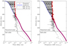 |
Fig. 3 Time delay (left panel) and frequency shift (right panel) due to the atmosphere of the occulting planet for an index of refraction profile given in Eq. (152a) with N0 = 10−6. Red circles represent results of the numerical integration (i.e., |


7.3 Accuracy of analytical solutions
We are now able to perform the comparison between analytical and numerical solutions for the time and frequency transfers considering the index of refraction profile given in Eq. (152a).
The analytical solution for the atmospheric time delay is constructed from the first-order delay function in Eq. (133), that is  . The summations over the index m are stopped for m = 10, but could have been stopped long before thanks to the small value of the coefficient for the expansion (e.g., for K = R, we have
  ). The analytical solution for the relative Doppler frequency shift is built from Eq. (158) with
  deduced from the first-order terms in Eqs. (137) and (139), and for m = 10 in Eq. (146). Because the receiver is at infinity, we replace xB with
 (160)
(160)
any time it appears in analytical expressions.
Results of the comparison are presented in Figs. 3 and 4 for N0 = 10−6 and 10−3, respectively.In both figures, we note that analytical solutions for the time and the frequency transfers succeed in perfectly reproducing the effects due to the vertical temperature variations (see e.g., signature at h ≃ 200 km in Figs. 2–4). Furthermore, the difference between the numerical and the analytical profiles remains at the level of the numerical noise as shown in Fig. 3.
In addition, in order to assess the legitimacy of the light-dragging effect we show, in each plot, the difference of the numerical solution with an additional analytical solution built by setting Ω = 0. It is clearly seen that neglecting the light-dragging effect drastically decreases the accuracy of the analytical solution (up to three orders of magnitude for the time delay and up to two orders of magnitude for the relative Doppler frequency shift).
In this work, we focus our attention on the explicit resolution of the first post-Minkowskian order (see Eq. (77a)) which corresponds to the well-known excess path delay when the velocity of the medium is neglected. The second-order term is composed of a second-order correction to the excess path delay and a geometric delay involving the derivative of the first-order delay function. The effect of these neglected second-order terms can be seen in Figs. 3 and 4 when the differences between the numerical and analytical solutions start to increase. For N0 = 10−6 in Fig. 3, the second-order effects show up starting from h ≃ 150 km and their influence increases when the altitude decreases, while they manifest at higher altitude, around h ≃ 250 km, for N0 = 10−3 in Fig. 4.
For N0 = 10−3, the differences between analytical solutions and numerical results are thus dominated by numerical noise above h ≃ 250 km and by the neglected second order below. The relative error has its minimum value of 0.001% for h ≃ 250 km and exceeds the 10% level below h ≃ 50 km for both the time delay and the relative Doppler frequency shift. This means that for high refractivity (i.e., N0 = 10−3) and for low altitude (i.e., h < 50 km), we cannot expect the first-order analytical solutions to describe the overall atmospheric effects with a relative accuracy better than one part in ten. In order to achieve a more accurate modeling, second-order terms (i.e., the second-order correction to the excess path delay and the geometric delay) shall be considered.
For N0 = 10−6 the relative error is dominated by numerical noise above h ≃ 150 km and by the neglected second order below. For h ≃ 150 km, the relative error is 0.001% and reaches 0.1% at the ground level for both the time delay and the relative Doppler frequency shift. This means that for small refractivity (i.e., N0 = 10−6), neglecting second-order terms would not make the relative errors larger than one part in 103 on the atmospheric time delay and the relative Doppler frequency shift retrievals. In that respect, the maximum absolute errors (at ground level) due to neglected second-order terms are expected to be at the level of 1 mm on the time delay and ![Mathematical equation: $10^{-13}\ [\nu_B]_{\mathrm{vac}}$](/articles/aa/full_html/2021/04/aa40269-20/aa40269-20-eq307.png) on the Doppler frequency shift.
on the Doppler frequency shift.
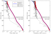 |
Fig. 4 Time delay (left panel) and frequency shift (right panel) due to the atmosphere of the occulting planet for an index of refraction profile given in Eq. (152a) with N0 = 10−3. The reader is referred to the caption of Fig. 3 for more details. |
8 Conclusions
In this workwe present a fully covariant analysis for deriving analytical expressions for the time and frequency transfers in the context of atmospheric occultation experiments. We combine two distinct relativistic theoretical tools, namely the Gordon’s optical metric and the time transfer functions formalism. We provide the integral form of the refractive delay function for any post-Minkowskian order and consider the case of an occultation by a steadily rotating and spherically symmetric atmosphere. We assume a refractivity profile driven by an exponential pressure profile and a polynomial temperature profile of arbitrary degree. We explicitly solve for the time and frequency transfers at first post-Minkowskian order in the limit where the angular velocity of the optical medium is small with respect to the speed of light in a vacuum. Finally, we assess the accuracy of the first-order analytical solutions by comparing them to results of a numerical integration of the equations for optical rays. We emphasize how complete these first-order analytical solutions actually are. Indeed, they are able to properly consider any vertical temperature gradients and properly account for light-dragging effect due to the motion of the optical medium. We also notice that for refractivity higher than 10−3, solutions that include up to the second post-Minkowskian order should be considered. The fully covariant method described in this paper can easily be extended in order to include following orders even beyond spherical symmetry. An immediate application of the analytical method presented in this paper is the assessment of the expected sensitivities in pressure, density, and temperature profiles for planetary atmospheric radio occultation experiments. This is beyond the scope of this paper and will be the subject of future research.
Finally, let us provide a guideline to make it easier to use our equations. The reader who is interested in deriving analytical expressions for the time and frequency transfers beyond the post-Minkowskian order can focus either on the integration of Eqs. (61) or (77) depending on whether the optical metric is static or stationary, respectively.
The reader who is interested in implementing the analytical expressions for the frequency transfer in a data analysis algorithm can proceed as follows. First, the coordinate time at emission (we focus on the case of a downlink one-way transfer here) shall be determined iteratively with the help of the time transfer function expression in Eq. (149) using the following algorithm:
![Mathematical equation: \begin{equation*} t_A^{[i]}\,{=}\,t_B-\mathcal{T}\big(\bm{x}_A(t_A^{[i-1]}),\bm{x}_B(t_B)\big) \qquad \mathrm{for}\ i>0\text{,} \end{equation*}](/articles/aa/full_html/2021/04/aa40269-20/aa40269-20-eq308.png) (161)
(161)
while ![Mathematical equation: $|t_A^{[i]}-t_A^{[i-1]}|>$](/articles/aa/full_html/2021/04/aa40269-20/aa40269-20-eq309.png) required precision, with
required precision, with
![Mathematical equation: \begin{equation*} t_A^{[0]}\,{=}\,t_B\text{.} \end{equation*}](/articles/aa/full_html/2021/04/aa40269-20/aa40269-20-eq310.png) (162)
(162)
If the refractivity of the atmosphere is not known, the delay function Δ(xA, xB) (cf. Eqs. (25) and (36)) can be set to zero. Otherwise, the values for the refractivity at ground level N0, the scale height H, and the polynomial coefficients bm can be directly substituted within Eq. (149). Then, when the coordinate time at emission is known, the position of the emitter xA(tA) can be determined, and hence, the frequency transfer can be eventually modeled after substituting  and
and  from Eqs. (150) into (136) and then (32). Thus, if the refractivity profile is known, the analytical expressions (150), (136), and (32) provide the frequency transfer directly. Otherwise, N0, H, and bm can be determined by minimizing the frequency transfer by using, for instance, a standard weighted least squares fit.
Acknowledgements
We thank the anonymous referee for comments. A.B., M.Z., L.G.C., and P.T. are grateful to the Italian Space Agency (ASI) for financial support through Agreement No. 2018-25-HH.0 in the context of ESA’s JUICE mission, and Agreement No. 2020-13-HH.0 in the context of TRIDENT’s mission Phase A study.
Appendix A Abel transform method
In this section, we show how the atmospheric time delay and the refractivity can both be directly inferred from real Doppler data by making use of an Abel transform method. The main novelty of the following approach lies in its consideration of the dragging of light due to the angular velocity of the rigid rotation of the atmosphere.
A.1 Bending angle from frequency transfer
A general expression for the frequency transfer can be inferred from Eqs. (136) and (137) such as
![Mathematical equation: \begin{equation*} \frac{\nu_B}{\nu_A}\,{=}\,\left[\frac{\nu_B}{\nu_A}\right]_{\mathrm{vac}}\left(\frac{1+\displaystyle\sum_{m\,{=}\,1}^{\infty}(N_0)^m\frac{\underline{\bm{l}}^{(m)}_B\cdot\bm{\beta}_B}{1+\bm{\beta}_B\cdot\underline{\bm{l}}_B^{\mathrm{(vac)}}}}{1+\displaystyle\sum_{m\,{=}\,1}^{\infty}(N_0)^m\frac{\underline{\bm{l}}^{(m)}_A\cdot\bm{\beta}_A}{1+\bm{\beta}_A\cdot\underline{\bm{l}}_A^{\mathrm{(vac)}}}}\right)\text{,} \end{equation*}](/articles/aa/full_html/2021/04/aa40269-20/aa40269-20-eq313.png) (A.1)
(A.1)
where the first factor on the right-hand side represents the frequency transfer in a vacuum, namely
![Mathematical equation: \begin{equation*} \left[\frac{\nu_B}{\nu_A}\right]_{\mathrm{vac}}\,{=}\,\frac{(u^0)_B}{(u^0)_A}\left(\frac{1+\bm{\beta}_B\cdot\underline{\bm{l}}_B^{\mathrm{(vac)}}}{1+\bm{\beta}_A\cdot\underline{\bm{l}}_A^{\mathrm{(vac)}}}\right)\text{.}\end{equation*}](/articles/aa/full_html/2021/04/aa40269-20/aa40269-20-eq314.png) (A.2a)
(A.2a)
The two triplets  and
and  represent the directions of the light ray in a vacuum at the emission and reception, that is to say

The omitted terms, proportional to G, represent the gravitational effects that are neglected here for clarity. The reader is referred to Linet & Teyssandier (2013) for a complete determination of the gravitational terms up to G3 in the context of a static, spherically symmetric spacetime.
For applications in the Solar System we can always consider that the 3-velocities are small with respect to the speed of light in a vacuum, that is to say ∥βA∥ and ∥βB∥≪ 1. Thus, at first order inN0, ∥βA ∥, and ∥βB ∥, we get
![Mathematical equation: \begin{equation*} \frac{\nu_B}{\nu_A}\,{=}\,\left[\frac{\nu_B}{\nu_A}\right]_{\mathrm{vac}}\left(1+N_0\,\underline{\bm{l}}^{(1)}_B\cdot\bm{\beta}_B-N_0\,\underline{\bm{l}}^{(1)}_A\cdot\bm{\beta}_A\right)\text{.} \end{equation*}](/articles/aa/full_html/2021/04/aa40269-20/aa40269-20-eq318.png) (A.3)
(A.3)
After substituting  and
and  from Eqs. (139), and making use of (145), the previous equation now reads
![Mathematical equation: \begin{equation*} \frac{\nu_B}{\nu_A}\,{=}\,\left[\frac{\nu_B}{\nu_A}\right]_{\mathrm{vac}}\left(1+N_0\,\phi^{(1)}\bm{n}_K\cdot\bm{\beta}_{\mathrm{eff}}\right)\text{,}\end{equation*}](/articles/aa/full_html/2021/04/aa40269-20/aa40269-20-eq321.png) (A.4)
(A.4)
where we introduce βeff, an effective velocity, such as
 (A.5)
(A.5)
Let us note that when the receiver is at infinity (as in one-way radio occultations by planets or satellites of the outer Solar System), wehave
 (A.6)
(A.6)
and therefore the effective velocity reduces to
 (A.7)
(A.7)
On the other hand, if the emitter is at infinity (like for one-way stellar occultations by planets or satellites of the Solar System), we have
 (A.8)
(A.8)
and therefore the effective velocity reduces to
 (A.9)
(A.9)
Equation (A.4) allows the first-order bending angle to be determined at each time step from real Doppler data. Because the impact parameter is only given by the geometry at a given time, the data eventually provide  .
.
A.2 Atmospheric time delay from bending angle
The refractive delay function can then be straightforwardly retrieved from the bending angle because, according to Eq. (145), the bending angle is the derivative of the delay function with respect to K.
At first post-Minkowskian order, we recall that the delay function and the bending angle (see Eqs. (52) and (144), respectively) are given by
 (A.10)
and
 (A.11)
Therefore, by making use of (145), we find
 (A.12)
where the constant of integration has been chosen such that
 (A.13)
considering that the bending angle is null at the beginning of the occultation, that is to say
 (A.14)
After determining  thanks to Eq. (A.4), Eq. (A.12) allows the atmospheric time delay and then the total light time to be determined.
A.3 Refractivity from bending angle
We see in Sect. 6.2 that  is defined by Eq. (123). If we apply the following change of variables

we can rewrite Eq. (123) as
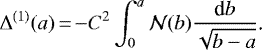 (A.16)
Interestingly, it can be seen that this expression is a special case of Abel transform (see e.g., Phinney & Anderson 1968; Landau & Lifshitz 1969), which allows us to write
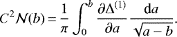 (A.17)
Going back to the previous set of variables, and making use of Eq. (145), we infer the following relationship after multiplying both sides of Eq. (A.17) by N0
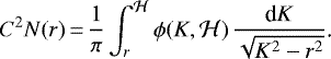 (A.18)
After integrating the right-hand side by parts we get
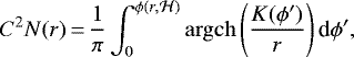 (A.19)
where we use (A.14) to show that
![Mathematical equation: \begin{equation*} \left[\phi(K,\mathcal{H})\,\mathrm{argch}\left(\frac{K}{r}\right)\right]_{K\,{=}\,r}^{K\,{=}\,\mathcal H}\,{=}\,0\text{.} \end{equation*}](/articles/aa/full_html/2021/04/aa40269-20/aa40269-20-eq340.png) (A.20)
(A.20)
The expression for C2 can be inferred from Eq. (122).
It is interesting to confront Eq. (A.19) with the standard Abel transform (Fjeldbo et al. 1971) which usually provides thefollowing expression
![Mathematical equation: \begin{equation*} n(r)\,{=}\,\exp\left[\frac{1}{\pi}\int^{\phi(r,\mathcal{H})}_{0}\mathrm{argch}\left(\frac{K(\phi')}{r}\right)\textrm{d}\phi'\right]\text{.}\end{equation*}](/articles/aa/full_html/2021/04/aa40269-20/aa40269-20-eq341.png) (A.21)
(A.21)
According to Eq. (4), in the limiting case where C2 → 1 (i.e., no light-dragging effect), it is seen that Eq. (A.19) corresponds to the first-order expression of Eq. (A.21). Thus, the novelty of Eq. (A.19) with respect to Eq. (A.21) lies in the fact that it takes into account the light-dragging effect through the geometric factor C2.
References
- Arfken, G. 1985, Mathematical Methods for Physicists, 3rd edn. (San Diego: Academic Press, Inc.) [Google Scholar]
- Blanchet, L., Salomon, C., Teyssandier, P., & Wolf, P. 2001, A&A, 370, 320 [NASA ADS] [CrossRef] [EDP Sciences] [Google Scholar]
- Born, M., & Wolf, E. 1999, Principles of Optics (Cambridge: Cambridge University Press, UK), 986 [Google Scholar]
- Bourgoin, A. 2020, Phys. Rev. D, 101, 064035 [Google Scholar]
- Bourgoin, A., Zannoni, M., & Tortora, P. 2019, A&A, 624, A41 [EDP Sciences] [Google Scholar]
- Brumberg, V. A. 1987, Kinematika i Fizika Nebesnykh Tel, 3, 8 [Google Scholar]
- Ehlers, J. 1967, Zeitschrift Naturforschung Teil A, 22, 1328 [Google Scholar]
- Fjeldbo, G., & Eshleman, V. R. 1965, J. Geophys. Res., 70, 3217 [Google Scholar]
- Fjeldbo, G., & Eshleman, V. R. 1968, Planet. Space Sci., 16, 1035 [Google Scholar]
- Fjeldbo, G., Kliore, A. J., & Eshleman, V. R. 1971, AJ, 76, 123 [Google Scholar]
- Gordon, W. 1923, Annalen der Physik, 377, 421 [Google Scholar]
- Hees, A., Lamine, B., Reynaud, S., et al. 2012, Class. Quantum Gravity, 29, 235027 [Google Scholar]
- Hees, A., Bertone, S., & Le Poncin-Lafitte, C. 2014, Phys. Rev. D, 89, 064045 [Google Scholar]
- Kliore, A., Cain, D. L., Levy, G. S., et al. 1965, Science, 149, 1243 [Google Scholar]
- Landau, L. D., & Lifshitz, E. M. 1960, Electrodynamics of Continuous Media (Amsterdam: Elsevier Science) [Google Scholar]
- Landau, L. D., & Lifshitz, E. M. 1969, Mechanics (Amsterdam: Elsevier Science) [Google Scholar]
- Le Poncin-Lafitte, C., Linet, B., & Teyssandier, P. 2004, Class. Quantum Gravity, 21, 4463 [Google Scholar]
- Lindal, G. F. 1992, AJ, 103, 967 [Google Scholar]
- Lindal, G. F., Sweetnam, D. N., & Eshleman, V. R. 1985, AJ, 90, 1136 [Google Scholar]
- Lindal, G. F., Lyons, J. R., Sweetnam, D. N., Eshleman, V. R., & Hinson, D. P. 1987, J. Geophys. Res., 92, 14987 [Google Scholar]
- Linet, B., & Teyssandier, P. 2002, Phys. Rev. D, 66, 024045 [Google Scholar]
- Linet, B., & Teyssandier, P. 2013, Class. Quantum Gravity, 30, 175008 [Google Scholar]
- Perlick, V. 2000, Ray Optics, Fermat’s Principle, and Applications to General Relativity (Berlin: Springer-Verlag) [Google Scholar]
- Phinney, R. A., & Anderson, D. L. 1968, J. Geophys. Res., 73, 1819 [Google Scholar]
- Poisson, E., & Will, C. M. 2014, Gravity (Cambridge: Cambridge University Press) [Google Scholar]
- Press, W. H., Teukolsky, S. A., Vetterling, W. T., & Flannery, B. P. 1992, Numerical Recipes in FORTRAN, The Art of Scientific Computing, 2nd ed. (Cambridge: Cambridge: University Press) [Google Scholar]
- Quan, P. M. 1957, Arch. Ration. Mech. Anal., 1, 54 [Google Scholar]
- Richter, G. W., & Matzner, R. A. 1983, Phys. Rev. D, 28, 3007 [Google Scholar]
- Roques, F., Sicardy, B., French, R. G., et al. 1994, A&A, 288, 985 [NASA ADS] [Google Scholar]
- Schinder, P. J., Flasar, F. M., Marouf, E. A., et al. 2012, Icarus, 221, 1020 [Google Scholar]
- Schinder, P. J., Flasar, F. M., Marouf, E. A., et al. 2015, Rad. Sci., 50, 712 [Google Scholar]
- Sicardy, B., Colas, F., Widemann, T., et al. 2006, J. Geophys. Res. Planets, 111, E11S91 [Google Scholar]
- Steiner, A. K., Kirchengast, G., & Ladreiter, H. P. 1999, Ann. Geophys., 17, 122 [Google Scholar]
- Synge, J. L. 1960, Relativity: the General Theory (Amsterdam: North-Holland Publ. Co.) [Google Scholar]
- Teyssandier, P. 2012, Class. Quantum Gravity, 29, 245010 [Google Scholar]
- Teyssandier, P., & Le Poncin-Lafitte, C. 2008, Class. Quantum Gravity, 25, 145020 [Google Scholar]
- Waite, J. H., Bell, J. M., Lorenz, R., Achterberg, R., & Flasar, F. M. 2012, Lunar Planet. Sci. Conf., 43, 1232 [Google Scholar]
- Withers, P. 2010, Adv. Space Res., 46, 58 [Google Scholar]
In this section, we use the convention that indices with a circumflex starting from the first part of the Greek or Latin alphabet denote components expressed in the rotating frame.
All Tables
Values of bm coefficients for the determination of a sixth-degree polynomial temperature profile.
All Figures
|
Fig. 1 Illustration of an occultation event in spacetime. The past light cone
|
| In the text | |
|
Fig. 2 Temperature profiles inside the atmosphere of the occulting planet. The plain curve represents a sixth-degree polynomial temperature profile, the dashed line represents an isothermal atmospheric profile, and the dotted line is the Titan atmospheric model of Waite et al. (2012). |
| In the text | |
|
Fig. 3 Time delay (left panel) and frequency shift (right panel) due to the atmosphere of the occulting planet for an index of refraction profile given in Eq. (152a) with N0 = 10−6. Red circles represent results of the numerical integration (i.e., |
| In the text | |
|
Fig. 4 Time delay (left panel) and frequency shift (right panel) due to the atmosphere of the occulting planet for an index of refraction profile given in Eq. (152a) with N0 = 10−3. The reader is referred to the caption of Fig. 3 for more details. |
| In the text | |
Current usage metrics show cumulative count of Article Views (full-text article views including HTML views, PDF and ePub downloads, according to the available data) and Abstracts Views on Vision4Press platform.
Data correspond to usage on the plateform after 2015. The current usage metrics is available 48-96 hours after online publication and is updated daily on week days.
Initial download of the metrics may take a while.