| Issue |
A&A
Volume 652, August 2021
|
|
|---|---|---|
| Article Number | A88 | |
| Number of page(s) | 7 | |
| Section | The Sun and the Heliosphere | |
| DOI | https://doi.org/10.1051/0004-6361/202038003 | |
| Published online | 13 August 2021 | |
Spatial variation in the periods of ion and neutral waves in a solar magnetic arcade
1
Center for Mathematical Plasma Astrophysics, Department of Mathematics, KU Leuven, Celestijnenlaan 200B, 3001 Leuven, Belgium
e-mail: This email address is being protected from spambots. You need JavaScript enabled to view it.
2
Institute of Physics, University of Maria Curie-Skłodowska, Pl. Marii Curie-Skłodowskiej 5, 20-031 Lublin, Poland
3
Department of Physics, University of Texas at Arlington, Arlington, TX 76019, USA
4
Leibniz-Institut für Sonnenphysik (KIS), Schöneckstr. 6, 79104 Freiburg, Germany
Received:
23
March
2020
Accepted:
10
May
2021
Abstract
Context. We present new insight into the propagation of ion magnetoacoustic and neutral acoustic waves in a magnetic arcade in the lower solar atmosphere.
Aims. By means of numerical simulations, we (a) study two-fluid waves propagating in a magnetic arcade embedded in the partially ionised, lower solar atmosphere and (b) investigate the effect of the background magnetic field configuration on the observed wave-periods.
Methods. We considered a 2D approximation of the gravitationally stratified and partially ionised lower solar atmosphere consisting of ion plus electron and neutral fluids that are coupled by ion-neutral collisions. In this model, the convection below the photosphere causes the excitation of ion magnetoacoustic-gravity and neutral acoustic-gravity waves.
Results. We find that in the solar photosphere, where ions and neutrals are strongly coupled by collisions, ion magnetoacoustic-gravity and neutral acoustic-gravity waves have periods ranging from 250 s to 350 s. In the chromosphere, where the collisional coupling is weak, the wave characteristics strongly depend on the magnetic field configuration. Above the footpoints of the considered arcade, the plasma is dominated by a vertical magnetic field along which ion magnetoacoustic-gravity waves propagate. These waves exhibit a broad range of periods, and the most prominent periods are 180 s, 220 s, and 300 s. Above the main loop of the solar arcade, where mostly horizontal magnetic field lines guide ion magnetoacoustic-gravity waves, the main spectral power reduces to the period of about 180 s, and no longer wave-periods exist.
Conclusions. In photospheric regions, ongoing solar granulation excites a broad spectrum of wave-periods that undergoes complex interactions: mode-coupling, refractions through the inhomogeneous atmosphere, real physical absorption, and conversion of wave power. We found that, in addition, the magnetic arcade configuration with a partially ionised plasma drastically changes the image of wave-periods observed in the upper layers of the chromosphere and corona. Our results agree with recent observational data.
Key words: Sun: activity / Sun: chromosphere / Sun: transition region / methods: numerical
© ESO 2021
1. Introduction
Plasma consisting of two fluids, namely ions plus electrons and neutrals, which are in a gravity-free and homogeneous equilibrium state and are permeated by a uniform magnetic field, can guide slow and fast ion magnetoacoustic waves (MAWs), and neutral acoustic waves, Alfvén waves, and entropy or thermal modes (e.g., Nakariakov & Verwichte 2005; Ballester et al. 2018). Small-amplitude Alfvén waves directly alter azimuthal (tangential-perpendicular) components of the ion velocity and magnetic field, while the other plasma quantities remain essentially unperturbed. Ion and neutral entropy or thermal modes correspond to non-propagating mass density perturbations (e.g., Goedbloed & Poedts 2004; Murawski et al. 2011). Neutral acoustic waves are coupled to ion MAWs through ion-neutral collisions. These waves are dispersive, and collisions introduce characteristic spatial and temporal scales (e.g., Zaqarashvili et al. 2011; Ballester et al. 2018). It is the subject of some on-going discussions whether two-fluid effects are negligible at low frequency (e.g., Soler et al. 2013, Ballai 2019, among others). Recently published results showed, however, that two-fluid effects play an important role even in the case of low-frequency waves when non-linear effects occur, especially in the context of wave damping and plasma heating (e.g., Kuźma et al. 2019, Wójcik et al. 2020, Murawski et al. 2020, Zhang et al. 2021).
In a gravitationally stratified atmosphere, internal gravity (henceforth “gravity”) waves join the above-mentioned waves. These gravity waves are unable to propagate along the vertical direction, but otherwise, they couple to acoustic waves or MAWs and create a hybrid entity called magnetoacoustic-gravity (MAG) waves (e.g., Vigeesh et al. 2017). In the extreme limit of an atmosphere free of magnetic field, the magnetic (slow MAWs and Alfvén) waves disappear and fast MAWs become purely acoustic (e.g., Nakariakov & Verwichte 2005).
Solar granulation operates within the lowest atmospheric layer, called the photosphere. It is a source of various dynamical events such as eddies, downdrafts, and the waves described above (e.g., Vigeesh et al. 2017). In a quiet photospheric region, the wave spectrum exhibits its main power at about a period of 300 s (e.g., Leighton et al. 1962; Christensen-Dalsgaard et al. 1991), and ions and neutrals are strongly coupled there by frequent collisions. However, in a magnetic flux-tube and in the chromosphere, the average period of the oscillations is close to 180 s (e.g., Deubner & Fleck 1990). As a result, the ion-neutral collision frequency decreases with height, and the ion-neutral coupling becomes weak in the upper chromosphere.
Several attempts have been made to explain the origin of the so-called “three-minute oscillations” (e.g., Lamb 1909, 1911; Moore & Spiegel 1964; Moore & Fung 1972; Ulmschneider et al. 1978; Cuntz et al. 1998; Fawzy et al. 2002; Musielak et al. 2006; Fawzy & Musielak 2012; Routh & Musielak 2014; Kraśkiewicz et al. 2019). In particular, Fleck & Schmitz (1993) compared four different spectra of injected waves at the lower boundary. They found that a shock-overtaking mechanism removes high-frequency waves, while essentially any driver results in three-minute chromospheric oscillations as a property of the stratification. Their results were confirmed within the framework of magnetohydrodynamic (MHD) and a two-fluid model by Kraśkiewicz et al. (2019) and Wójcik et al. (2018), respectively, who additionally showed that ions and neutrals oscillate differently, while being excited by a monochromatic driver in an atmosphere free of magnetic field. The case of a strong magnetic field was discussed by Botha et al. (2011), who observed three-minute oscillations in the chromosphere above sunspot umbrae and developed a model based on ideal MHD equations with a uniform vertical background magnetic field and a temperature profile corresponding to sunspot atmospheres. The long wave-periods in the spectrum of the broadband pulse were filtered out so that wave-periods below the acoustic cutoff wave-period resonated inside the chromospheric cavity with about three minutes.
Recently, Wójcik et al. (2018) performed two-fluid numerical simulations of a partially ionised solar atmosphere that is permeated by a weak and initially vertical magnetic field. They concluded that MAWs that are excited by granulation convert their main power from a period of about 300 s in the photosphere into oscillations of about 220 s in the chromosphere.
The main goal of the present paper is to generalise the two-fluid models presented by Wójcik et al. (2018) and Wójcik et al. (2019) to a magnetic arcade that contains regions of a weak horizontal magnetic field that interacts with ion MAG waves, and two zones of stronger, mostly vertical magnetic field that acts like a wave guide. The obtained results discover the role of waves in transporting energy from the solar photosphere to the upper layers of the solar chromosphere, heating the latter, and the effects of cutoff frequencies on the propagation of these waves. The results of our numerical simulations are compared to observational data given by Wiśniewska et al. (2016) and Kayshap et al. (2018) and agree well.
In the following section the two-fluid equations are presented and discussed. Section 3 contains a presentation of the results of the numerical simulations, and in Sect. 4 the main results are summarised.
2. Two-fluid equations
We used the two-fluid equations in which (ioni and neutraln) mass densities, 𝜚i, n, velocities, Vi, n, (ion plus electronie and neutraln) gas pressures, pi e, n, and the magnetic field B evolve according to (e.g., Oliver et al. 2016; Ballester et al. 2018)
 (1)
(1)
 (2)
(2)
![Mathematical equation: $$ \begin{aligned}&\frac{\partial E_{\rm n}}{\partial t}+\nabla \cdot [(E_{\rm n}+p_{\rm n})\mathbf V _{\rm n}] = \alpha _{\rm in}\mathbf V _{\rm n}\cdot (\mathbf{V}_{\rm i}-\mathbf{V}_{\rm n})\nonumber \\&\qquad \ \ \qquad \qquad \qquad \qquad +Q_{\rm n} ^\mathrm{in} + \varrho _{\rm n} \mathbf g \cdot \mathbf V _{\rm n}, \end{aligned} $$](/articles/aa/full_html/2021/08/aa38003-20/aa38003-20-eq3.gif) (3)
(3)
where the heat production and exchange term for neutrals is given by
![Mathematical equation: $$ \begin{aligned} Q_{\rm n}^\mathrm{in} = \alpha _{\rm in} \left[\frac{1}{2} |\mathbf{V }_{\rm i}-\mathbf{V }_{\rm n} |^2 + \frac{3k_{\rm B}}{m_{\rm H}(\mu _{\rm i}+\mu _{\rm n})}\left(T_{\rm i}-T_{\rm n} \right)\right], \end{aligned} $$](/articles/aa/full_html/2021/08/aa38003-20/aa38003-20-eq4.gif) (4)
(4)
and the neutral (internal + kinetic) energy density is defined as
 (5)
(5)
For an ion plus electron mixture, we used the following set of MHD equations:
 (6)
(6)
 (7)
(7)
 (8)
(8)
![Mathematical equation: $$ \begin{aligned}&\frac{\partial E_{\rm i}}{\partial t}+\nabla \cdot \left[\left(E_{\rm i}+p_{\rm ie} + \frac{|\mathbf B |^2}{2\mu _0}\right)\mathbf V _{\rm i}- \frac{1}{\mu _0}\mathbf B (\mathbf V_{\rm i} \cdot \mathbf B )\right] \nonumber \\&\qquad \qquad \qquad = \alpha _{\rm in}\mathbf V _{\rm i}\cdot (\mathbf{V}_{\rm n}-\mathbf{V}_{\rm i}) + Q_{\rm i}^\mathrm{in} + \varrho _{\rm i} \mathbf g \cdot \mathbf V _{\rm i}+L_{\rm r}, \end{aligned} $$](/articles/aa/full_html/2021/08/aa38003-20/aa38003-20-eq9.gif) (9)
(9)
with a similar heat exchange and production term for ions given by
![Mathematical equation: $$ \begin{aligned} Q_{\rm i}^\mathrm{in} = \alpha _{\rm in} \left[\frac{1}{2} |\mathbf{V }_{\rm i}-\mathbf{V }_{\rm n} |^2 + \frac{3k_{\rm B}}{m_{\rm H}(\mu _{\rm i}+\mu _{\rm n})}\left(T_{\rm n}-T_{\rm i} \right)\right], \end{aligned} $$](/articles/aa/full_html/2021/08/aa38003-20/aa38003-20-eq10.gif) (10)
(10)
and the ion (internal + kinetic + magnetic) energy density defined as
 (11)
(11)
Here, g = [0, −g, 0] is a gravity vector with a magnitude g = 274.78 m s−2, αin denotes the coefficient of collisions between ion and neutral particles (e.g., Ballester et al. 2018 and references cited therein), μi = 0.58 and μn = 1.21 are the mean masses of ions and neutrals, respectively, which are specified by the OPAL solar abundance model, while mH is the hydrogen mass, kB is the Boltzmann constant, and γ = 1.4 is the specific heat ratio. Oliver et al. (2016) assumed hydrogen plasma, thus they implied μi ≈ μn in Eqs. (4) and (10). The symbol Lr denotes the radiative loss term, which consists of two separate parts: thick cooling that operates in the low atmospheric layers, and thin cooling that works in the upper atmospheric regions. At every time step, we calculated the optical depth starting at infinity and ending at the bottom boundary. For optical depths higher than 0.1, we used the thick cooling approximation of Abbett & Fisher (2011). For optical depths lower than 0.1, we used thin cooling (Moore & Fung 1972). The other symbols in Eqs. (1)–(11) have their standard meaning. The pressures of ions plus electrons and neutrals are given by the ideal gas laws as
 (12)
(12)
After specifying the temperature profile and using Eqs. (1)–(12), we obtained the hydrostatic ion and neutral mass densities and the gas pressure profiles. As a result of the low mass of electrons in comparison to ions and neutrals, we neglected all electron-associated terms in the induction equation (Ballester et al. 2018) and also all terms corresponding to viscosity, magnetic resistivity, ionisation, and recombination. These terms and effects will be included in future studies.
3. Numerical simulations and results
3.1. Numerical set up, boundary, and initial conditions
To solve the two-fluid equations numerically, we used the code JOANNA (Wójcik et al. 2018, 2019), which solves the two-fluid equations in the form (1)–(12). In our numerical experiments, we set the Courant-Friedrichs-Lewy (Courant et al. 1928) number equal to 0.9 and chose a second-order accuracy in space and a four-stage, third-order strong stability preserving Runge-Kutta method (Durran 2010) for integration in time, supplemented by adopting the Harten-Lax-van Leer Discontinuities (HLLD) approximate Riemann solver (Miyoshi et al. 2010) and the divergence of the magnetic field cleaning method of Dedner et al. (2002).
The two-dimensional simulation box is specified as −10.24 Mm < x < 10.24 Mm along the horizontal (x-) direction. In the vertical (y-) direction, the region from y = −2.56 Mm up to y = 7.68 Mm is covered by a uniform grid of cell size Δx = Δy = 20 km. Above this uniform-grid zone, a region of the stretched grid is implied up to y = 60 Mm and is covered by 128 cells. With the use of this non-uniform grid, any incoming signal is damped close to the upper boundary. It has been found that such stretched grid significantly reduces spurious reflections of the incoming signal (e.g., Kuźma & Murawski 2018). The size of the 128 stretched numerical cells grows with height. Thus, cells close to the area with a uniform grid have a similar size, and the transition from a uniform to a fully stretched grid is smooth and does not have any significant effect on propagating waves. The implemented grid resolves all spatial structures well, particularly those associated with solar granulation.
At the top and bottom boundaries, we fixed all plasma quantities, except for the ion and the neutral velocity, to their equilibrium values. Holding them fixed allowed us to reduce numerical noise due to the integration of the gravity term as well as numerically induced reflections of the incoming signal. At the lateral sides, periodic boundary conditions were implemented. The physical system was taken to be invariant along the z-direction (with ∂/∂z = 0), and Vz = Bz = 0 was set throughout the whole time. As a result of this, Alfvén waves were removed from the system, which still allowed MAG waves to propagate. Without implementing any transversal velocity perturbation, this condition is maintained self-consistently.
At t = 0 s, we set all plasma quantities to their hydrostatic values specified by the temperature given by the semi-empirical model of Avrett & Loeser (2008; Fig. 1, top). The equilibrium magnetic field was taken to be in the form of an arcade with its footpoints settled at x = −5.12 Mm and x = 5.12 Mm (Low 1985). The horizontal, Bx, vertical, By, and transversal, Bz , components of magnetic field are described by
 (13)
(13)
Here a1 = −5.12 Mm, a2 = 5.12 Mm and b = −2.8 Mm indicate locations of the magnetic singularities, and S denotes their strength in such a way that at the reference point yr = 6 Mm magnetic field strength equals B = 2 Gs. The term “magnetic arcade” typically refers to an active region structure; for the quiet Sun, the described magnetic configuration may represent a bipolar region of the network magnetic field. The magnitude of the magnetic field, B, reaches 100 G at the footpoints of the magnetic structure, and the magnetic field lines are essentially vertical there. Higher up, B declines with height. Between the footpoints of the magnetic arcade, the magnetic field lines become horizontal. The initial magnetic configuration is shown in Fig. 1(top). The bottom panel of Fig. 1 illustrates the resulting spatial profile of the plasma beta given by
 (14)
(14)
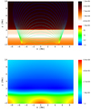 |
Fig. 1. Initial spatial profiles of logarithm of the ion temperature, Ti, expressed in K, overlaid with the magnetic field lines with the magnitude of the magnetic field, B, expressed in G (top) and logarithm of the plasma beta (bottom). |
3.2. Numerical experiments
We perturbed the magnetohydrostatic equilibrium with a very small random signal in the ion and neutral velocities to seed convection below the bottom of the solar photosphere, which is located at y = 0 Mm. As a result of this initial perturbation, the convection cells started forming and were already discernible after about 10 min of physical time, and fully developed convection occurred after about 1 h.
To sustain the ongoing convection, the problem of mass and energy losses was fixed in two ways. A plasma inflow at the bottom boundary was implemented in its vertical velocity component equal to 0.3 km s−1. This allowed us to compensate for the outflowing plasma mass and its energy losses. Additionally, the convection zone (y < 0 Mm) was heated by implementing an additional source term in the ion energy equation, which is higher than the radiative cooling term by 10% there. This source term mimics the plasma heating that results from the convection zone. These two values were calculated by assuming that the incoming flux and heating from below the simulation region compensate for the mass and energy losses and allow us to sustain an atmospheric quasi-equilibrium (Wójcik et al. 2020; Murawski et al. 2020).
Figure 2 illustrates the magnetic solar arcade perturbed by ion MAG and neutral acoustic-gravity waves excited by the ongoing solar convection and granulation at t = 3800 s, t = 4000 s, and t = 4200 s (from top to bottom). The colour map in the left panels shows the logarithm of the ion temperature, Ti, expressed in K, and the solid lines represent magnetic field lines. The well-developed granulation pattern operates in and below the photosphere, located approximately between y = 0 Mm and y = 0.5 Mm. Characteristic features of this granulation such as turbulence with strong downdrafts and weak upflows as well as a diversity of waves and flows are clearly visible. From Fig. 2 we infer that dense chromospheric plasma fills the structure of the magnetic solar arcade. On either side of this structure, namely at the footpoints of the magnetic arcade, located at x ≅ −5.12 and x ≅ 5.12 Mm, magnetic field lines form flux tubes. We note well-developed magnetic blobs rising from below the photosphere. The right panels of Fig. 2 illustrate the corresponding ion-neutral drift, |Vi − Vn|, expressed in km s−1 at the same three instants of time. As expected, both fluids are strongly coupled in the photosphere, but decouple in the chromosphere. This decoupling is especially well visible in the magnetic structure of the arcade, where the ion-neutral drift reaches its maximum value of tens of kilometers per second. The magnetic field, mostly horizontal here, does not directly affect the propagating neutral acoustic-gravity waves, while the ion magnetoacoustic-gravity waves propagating upwards do encounter its effect. A part of the energy carried by these waves is thermalised by the process of ion-neutral collisions (e.g., Kuźma et al. 2019). Higher up, in the solar corona, the ion-neutral drift loses its importance as plasma is in general fully ionised there.
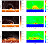 |
Fig. 2. Spatial profiles of logarithm of the ion temperature, Ti, expressed in K, overlaid with the magnetic field lines (left) and the corresponding ion-neutral drift, |Vi − Vn|, expressed in km s−1 (right) at t = 3800 s, t = 4000 s, and t = 4200 s (from top to bottom). |
Figure 3 displays a time-distance plot for the vertical component of the ion velocity collected at x = 0 Mm in the y-direction. Because at this location, the magnetic field lines are essentially horizontal, Vi y(x = 0, y, t) mainly corresponds to MAWs with a cut-off period Pk = 230 s. They were studied analytically by Stark & Musielak (1993) and numerically by Kraśkiewicz et al. (2019). Within the MHD model, Kraśkiewicz et al. (2019) showed that a monochromatic driver with a period of 300 s excites fast MAWs whose wave-period decreases to about 200 s at y ≈ 1 Mm. The oscillations with P = 200 s propagate essentially freely through the chromosphere, reaching the corona with the same period; see Fig. 5 in Kraśkiewicz et al. (2019). In the essentially horizontal magnetic field above the magnetic arcade, we observe plasma outflows with a vertical plasma velocity up to 60 km s−1. These outflows are significantly slower than the fast plasma outflows in the vertical magnetic field case (Wójcik et al. 2019).
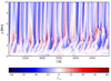 |
Fig. 3. Time-distance plot for Vi y(x = 0, y, t), given in units of 1 km s−1. |
Figure 4 illustrates the Fourier power spectrum of wave-period P associated with the ion vertical velocity, collected in time along the vertical line, given by x = 0 Mm. For x = 0 Mm, the magnetic field lines are essentially horizontal, and P is close to 227 s for all heights within the range of 1 Mm < y < 2 Mm. Higher up, for y > 2.1 Mm, the signal associated with P ≈ 227 s decays and the dominant wave-period is associated with P ≈ 167 s.
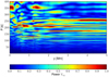 |
Fig. 4. Fourier power spectrum (in arbitrary units) of the wave-period P associated with the Vi y(x = 0, y, t) vs height y in the solar atmosphere. |
Figure 5 shows the dominant wave-periods obtained from the Fourier power spectrum for the vertical component of the ion velocity and the observational data collected by Wiśniewska et al. (2016) and Kayshap et al. (2018). We infer that the wave-period P follows the observational data, and conclude that the description of the solar atmospheric plasma in the framework of two-fluid equations for ions and neutrals agrees well for numerically detected periods of the waves, which are generated by the solar granulation and the observational data.
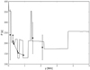 |
Fig. 5. Main wave-periods evaluated from Fourier power spectrum for the numerically obtained Vi y(x = 0, y, t) (solid black line) vs height. The diamonds and dots show the observational data by Wiśniewska et al. (2016) and Kayshap et al. (2018), respectively. The error bars for the dots represent the range of periods detected by these observations at three given heights. |
Figure 6 displays Fourier power spectrum of the ion velocity, collected along the horizontal lines, given by y = 0.25 Mm (top) and y = 3.5 Mm (bottom). We infer that the ongoing convective motions below the photosphere generate a broad range of wave-periods that can be observed at the top of the photosphere; the obtained Fourier power is highest between the wave-periods 250 s and 350 s. While propagating upwards, these waves are subject to complex interactions: mode-coupling, refractions through the inhomogeneous atmosphere, real physical absorption and conversion of wave power (e.g., Khomenko et al. 2018). Above the footpoints of the arcade, additional shorter wave-periods of 180 s and 220 s are generated. Above the main loop of the solar arcade, which is for −5.12 Mm < x < 5.12 Mm, where mostly horizontal magnetic field lines significantly interact with ion waves, the main spectral power drops to a period of about 180 s, and longer wave-periods are essentially non-existent.
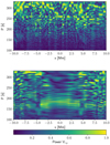 |
Fig. 6. Fourier power spectrum of P (in arbitrary units) associated with the vertical component of the ion velocity, evaluated at y = 0.25 Mm (top) and y = 3.5 Mm (bottom), vs horizontal distance x in the solar atmosphere. |
4. Summary
We performed 2D numerical simulations of two-fluid ion magnetoacoustic-gravity and neutral acoustic-gravity waves, which are generated by the solar granulation present in low regions of the solar atmosphere. This atmosphere is partially ionised with dynamic ions plus electrons and neutrals treated as separate fluids (e.g., Oliver et al. 2016; Ballester et al. 2018), and it is assumed to be initially permeated by a magnetic arcade. The fluids were described by magnetohydrodynamic (for ions plus electrons) and hydrodynamic (for neutrals) equations, which were coupled by collision terms and contain radiation terms corresponding to optically thick and thin cooling (Abbett & Fisher 2011). The solar granulation, which is generated in the system as a result of convective instability, excites various waves (e.g., Vigeesh et al. 2017) that are subject to the interaction with the magnetic field embedded in the stratified solar atmosphere, cut-off frequencies, and an enhancement in high-frequency acoustic power in the solar photosphere and the chromosphere surrounding magnetic active regions. Moreover, Rijs et al. (2015, 2016) reported the formation of an acoustic halo caused by MHD mode conversion through regions of moderate and inclined magnetic fields. This conversion type is most efficient when high-frequency waves from below intersect magnetic field lines at a large angle.
The main finding of this paper is that in the photospheric regions of highly turbulent and strongly coupled plasma the main period of excited waves is close to 300 s, while in the chromosphere, where both fluids decouple, the situation differs between regions outside and inside of the solar magnetic arcade. We showed that in these magnetic structures, a strong ion-neutral drift is present, while outside of these structures, ions and neutrals remain essentially coupled. In addition, refraction and subsequent reflection of magneto-acoustic waves around the regions of β = 1 (Rajaguru et al. 2013) significantly alter the wave propagation in this model. The waves become evanescent as a result of strong reflection in the inhomogeneous solar atmosphere, they decay with height, and may transfer their energy into the waves whose wave-periods are close to three minutes, which is seen above the solar arcade, while longer wave-periods propagate outside of the structure of the arcade. This agrees with findings of Rajaguru et al. (2019), who showed that less inclined magnetic field elements in the quiet Sun channel a significant number of waves with a frequency lower than the theoretical minimum acoustic cut-off frequency to the upper atmospheric layers. This also agrees well with the observations reported by Wiśniewska et al. (2016) and Kayshap et al. (2018).
Our results have important implications for the wave energy transfer in the solar atmosphere and its local wave heating, which still remains an unsolved problem in solar physics. Fleck et al. (2021) have recently compared ten different 3D magnetoconvection simulations from four different codes, namely Bifrost, CO5BOLD, MANCHA3D, and MURaM, with a variety of approximations, and described waves that are generated within them and how they varied with height. They found considerable differences between the various models. The height dependence of the wave power, in particular, of high-frequency waves, varies by up to two orders of magnitude, and the phase difference spectra of several models show unexpected features, including ∓180° phase jumps. Overall, several two-fluid effects included in our model will need separate dedicated studies using less complicated and idealised modelling techniques that will allow further comparison and verification.
Acknowledgments
This work was supported through the projects of National Science Centre (NCN), Poland, grant nos. 2017/25/B/ST9/00506, 2017/27/N/ST9/01798, 2020/37/B/ST9/00184, and C14/19/089 (C1 project Internal Funds KU Leuven), G.0D07.19N (FWO-Vlaanderen), SIDC Data Exploitation (ESA Prodex-12). This project (EUHFORIA 2.0) has received funding from the European Union’s Horizon 2020 research and innovation programme under grant agreement No 870405.
References
- Abbett, W. P., & Fisher, G. H. 2011, Sol. Phys., 277, 3 [NASA ADS] [CrossRef] [Google Scholar]
- Avrett, E., & Loeser, R. 2008, ApJS, 175, 229 [NASA ADS] [CrossRef] [Google Scholar]
- Ballai, I. 2019, Front. Astron. Space Sci., 6, 39 [CrossRef] [Google Scholar]
- Ballester, J. L., Alexeev, I., Collados, M., et al. 2018, Space Sci. Rev., 214, 58 [Google Scholar]
- Botha, G. J. J., Arber, T. D., Nakariakov, V. M., & Zhugzhda, Y. D. 2011, ApJ, 728, 84 [Google Scholar]
- Christensen-Dalsgaard, J., Gough, D. O., & Thompson, M. J. 1991, ApJ, 378, 413 [NASA ADS] [CrossRef] [Google Scholar]
- Courant, R., Friedrichs, K., & Lewy, H. 1928, Math. Ann., 100, 32 [NASA ADS] [CrossRef] [MathSciNet] [Google Scholar]
- Cuntz, M., Ulmschneider, P., & Musielak, Z. 1998, ApJ, 493, L117 [NASA ADS] [CrossRef] [Google Scholar]
- Dedner, A., Kemm, F., Kröner, D., et al. 2002, J. Comput. Phys., 175, 645 [Google Scholar]
- Deubner, F.-L., & Fleck, B. 1990, A&A, 228, 506 [NASA ADS] [Google Scholar]
- Durran, D. R. 2010, Numerical Methods for Fluid Dynamics (New York: Springer) [CrossRef] [Google Scholar]
- Fawzy, D. E., & Musielak, Z. E. 2012, MNRAS, 159 [Google Scholar]
- Fawzy, D., Rammacher, W., Ulmschneider, P., Musielak, Z. E., & Stępień, K. 2002, A&A, 386, 971 [NASA ADS] [CrossRef] [EDP Sciences] [Google Scholar]
- Fleck, B., Carlsson, M., Khomenko, E., et al. 2021, Phil. Trans. R. Soc. London, Ser. A, 379, 20200170 [Google Scholar]
- Fleck, B., & Schmitz, F. 1993, A&A, 273, 671 [NASA ADS] [Google Scholar]
- Goedbloed, J. P. H., & Poedts, S. 2004, Principles of Magnetohydrodynamics (Cambridge University Press) [CrossRef] [Google Scholar]
- Kayshap, P., Murawski, K., Srivastava, A. K., Musielak, Z. E., & Dwivedi, B. N. 2018, MNRAS, 479, 5512 [NASA ADS] [CrossRef] [Google Scholar]
- Khomenko, E., Vitas, N., Collados, M., & de Vicente, A. 2018, A&A, 618, A87 [NASA ADS] [CrossRef] [EDP Sciences] [Google Scholar]
- Kraśkiewicz, J., Murawski, K., & Musielak, Z. E. 2019, A&A, 623, A62 [NASA ADS] [CrossRef] [EDP Sciences] [Google Scholar]
- Kuźma, B., & Murawski, K. 2018, ApJ, 866, 50 [CrossRef] [Google Scholar]
- Kuźma, B., Wójcik, D., & Murawski, K. 2019, ApJ, 878, 81 [NASA ADS] [CrossRef] [Google Scholar]
- Lamb, H. 1909, Proc. London Math. Soc., s2-7, 122 [CrossRef] [Google Scholar]
- Lamb, H. 1911, Proc. London Math. Soc. A, 84, 551 [Google Scholar]
- Leighton, R. B., Noyes, R. W., & Simon, G. W. 1962, ApJ, 135, 474 [NASA ADS] [CrossRef] [Google Scholar]
- Low, B. C. 1985, ApJ, 293, 31 [NASA ADS] [CrossRef] [Google Scholar]
- Miyoshi, T., Terada, N., Matsumoto, Y., et al. 2010, IEEE Trans. Plasma Sci., 38, 9 [NASA ADS] [CrossRef] [Google Scholar]
- Moore, D., & Spiegel, E. 1964, ApJ, 139, 48 [NASA ADS] [CrossRef] [Google Scholar]
- Moore, R. L., & Fung, P. C. W. 1972, Sol. Phys., 23, 78 [NASA ADS] [CrossRef] [Google Scholar]
- Murawski, K., Musielak, Z. E., & Wójcik, D. 2020, ApJ, 896, L1 [CrossRef] [Google Scholar]
- Murawski, K., Zaqarashvili, T. V., & Nakariakov, V. M. 2011, A&A, 533, A18 [NASA ADS] [CrossRef] [EDP Sciences] [Google Scholar]
- Musielak, Z. E., Musielak, D. E., & Mobashi, H. 2006, Phys. Rev. E, 73, 036612 [NASA ADS] [CrossRef] [Google Scholar]
- Nakariakov, V. M., & Verwichte, E. 2005, Liv. Rev. Sol. Phys., 2 [Google Scholar]
- Oliver, R., Soler, R., Terradas, J., & Zaqarashvili, T. V. 2016, ApJ, 818, 128 [NASA ADS] [CrossRef] [Google Scholar]
- Rajaguru, S. P., Couvidat, S., Sun, X., Hayashi, K., & Schunker, H. 2013, Sol. Phys., 287, 107 [CrossRef] [Google Scholar]
- Rajaguru, S. P., Sangeetha, C. R., & Tripathi, D. 2019, ApJ, 871, 155 [NASA ADS] [CrossRef] [Google Scholar]
- Rijs, C., Moradi, H., Przybylski, D., & Cally, P. S. 2015, ApJ, 801, 27 [NASA ADS] [CrossRef] [Google Scholar]
- Rijs, C., Rajaguru, S. P., Przybylski, D., et al. 2016, ApJ, 817, 45 [NASA ADS] [CrossRef] [Google Scholar]
- Routh, S., & Musielak, Z. E. 2014, Astron. Nachr., 335, 1043 [NASA ADS] [CrossRef] [Google Scholar]
- Soler, R., Carbonell, M., & Ballester, J. L. 2013, ApJS, 209, 16 [NASA ADS] [CrossRef] [Google Scholar]
- Stark, B. A., & Musielak, Z. E. 1993, ApJ, 409, 450 [Google Scholar]
- Ulmschneider, R., Schmitz, F., Kalkofen, W., & Bohn, H. 1978, A&A, 70, 487 [Google Scholar]
- Vigeesh, G., Jackiewicz, J., & Steiner, O. 2017, ApJ, 835, 148 [NASA ADS] [CrossRef] [Google Scholar]
- Wiśniewska, A., Musielak, Z. E., Staiger, J., & Roth, M. 2016, ApJ, 819, L23 [Google Scholar]
- Wójcik, D., Murawski, K., & Musielak, Z. E. 2018, MNRAS, 481, 262 [NASA ADS] [CrossRef] [Google Scholar]
- Wójcik, D., Kuźma, B., Murawski, K., & Srivastava, A. K. 2019, ApJ, 884, 127 [CrossRef] [Google Scholar]
- Wójcik, D., Kuźma, B., Murawski, K., & Musielak, Z. E. 2020, A&A, 635, A28 [CrossRef] [EDP Sciences] [Google Scholar]
- Zaqarashvili, T. V., Khodachenko, M. L., & Rucker, H. O. 2011, A&A, 529, A82 [NASA ADS] [CrossRef] [EDP Sciences] [Google Scholar]
- Zhang, F., Poedts, S., Lani, A., Kuźma, B., & Murawski, K. 2021, ApJ, 911, 119 [CrossRef] [Google Scholar]
All Figures
|
Fig. 1. Initial spatial profiles of logarithm of the ion temperature, Ti, expressed in K, overlaid with the magnetic field lines with the magnitude of the magnetic field, B, expressed in G (top) and logarithm of the plasma beta (bottom). |
| In the text | |
|
Fig. 2. Spatial profiles of logarithm of the ion temperature, Ti, expressed in K, overlaid with the magnetic field lines (left) and the corresponding ion-neutral drift, |Vi − Vn|, expressed in km s−1 (right) at t = 3800 s, t = 4000 s, and t = 4200 s (from top to bottom). |
| In the text | |
|
Fig. 3. Time-distance plot for Vi y(x = 0, y, t), given in units of 1 km s−1. |
| In the text | |
|
Fig. 4. Fourier power spectrum (in arbitrary units) of the wave-period P associated with the Vi y(x = 0, y, t) vs height y in the solar atmosphere. |
| In the text | |
|
Fig. 5. Main wave-periods evaluated from Fourier power spectrum for the numerically obtained Vi y(x = 0, y, t) (solid black line) vs height. The diamonds and dots show the observational data by Wiśniewska et al. (2016) and Kayshap et al. (2018), respectively. The error bars for the dots represent the range of periods detected by these observations at three given heights. |
| In the text | |
|
Fig. 6. Fourier power spectrum of P (in arbitrary units) associated with the vertical component of the ion velocity, evaluated at y = 0.25 Mm (top) and y = 3.5 Mm (bottom), vs horizontal distance x in the solar atmosphere. |
| In the text | |
Current usage metrics show cumulative count of Article Views (full-text article views including HTML views, PDF and ePub downloads, according to the available data) and Abstracts Views on Vision4Press platform.
Data correspond to usage on the plateform after 2015. The current usage metrics is available 48-96 hours after online publication and is updated daily on week days.
Initial download of the metrics may take a while.