© The Authors 2025

1. Introduction

Dark energy and dark matter constitute the majority of the energy budget of our Universe (Planck Collaboration VI 2020). More precisely, dark energy causes the present-time cosmic acceleration (Perlmutter et al. 1998, 1999; Riess et al. 1998; Tonry et al. 2003; Bridle et al. 2003; Bennett et al. 2003; Hinshaw et al. 2003; Kogut et al. 2003; Spergel et al. 2003; Eisenstein et al. 2005) and exhibits repulsive effects (Luongo & Quevedo 2014), while dark matter plays a crucial role in the clustering of cosmic structure (Luongo 2025; Bergstrom 2009; Profumo et al. 2019). However, their fundamental nature is still the object of heated debate.

In the quest for understanding dark energy, various hypotheses have been put forth that all sought to determine whether its equation of state changes with the time (Chevallier & Polarski 2001; Linder 2003; Peebles & Ratra 2003; King et al. 2014) or if it remains a pure cosmological constant Λ (Padmanabhan 2003). The latter is generally associated with the effects of primordial quantum fluctuations and represents the key ingredient of the standard background scenario, namely the ΛCDM model (Sahni & Starobinsky 2000; Copeland et al. 2006; Tsujikawa 2011). This is essentially based on six free parameters (Planck Collaboration VI 2020; Perivolaropoulos & Skara 2022), with the further assumption of a flat topology, as supported by various observations (Efstathiou & Gratton 2020). However, the precise determination of the spatial curvature Ω_k still remains an open challenge in cosmology (Ooba et al. 2018).

For its theoretical structure, the ΛCDM model seems to be statistically favored to frame the dark energy dynamics, especially at late and early times. However, cosmological tensions and conceptual issues have recently been raised (Hu & Wang 2023), as has evidence in favor of an evolving dark energy even at late times (DESI Collaboration 2025). Different perspectives about the extensions of the standard model have been discussed, e.g., in Luongo & Muccino (2018), D’Agostino et al. (2022), Belfiglio et al. (2023).

Consequently, the use of additional standard candles, such as type Ia supernovae (SNe Ia, Scolnic et al. 2018), and/or standard rulers, such as baryonic acoustic oscillations (BAOs, Cuceu et al. 2019), may be not enough to determine whether dark energy is dynamical. Hence, intermediate- and high-redshift catalogs beyond the SN Ia detectability (Rodney et al. 2015) appear to be crucial to really understand whether the ΛCDM model may be seen as a limiting case of a more general paradigm (Capozziello et al. 2019, 2020).

Accordingly, GRBs are currently inspected as potential distance indicators (Muccino et al. 2021; Cao et al. 2022; Luongo & Muccino 2021a; Dainotti et al. 2022; Jia et al. 2022). Particularly, GRBs may crucially detect deviations from the well-established ΛCDM predictions. This would clarify the nature of the aforementioned cosmological tensions.

We explore whether GRBs can be used to detect limits on the equivalence between dark energy and additional cosmic fluids. Precisely, while the equivalence between matter and radiation applies to very high redshifts and culminates in the equivalence epoch, it is challenging to directly constrain either the equivalence between dark energy and radiation or dark energy and matter with radiation. We stress that the matter–radiation equivalence represents a cosmological epoch, that is, a time before which radiation dominated other fluids, while equating dark energy with radiation or with radiation plus matter provides cosmographic redshifts, without implying a time of domination of one of the two species. With existing data, these two equivalence times and their corresponding formal periods can be tentatively constrained, and because they are influenced by the dark energy form and free parameters, they can be used to directly distinguish among dark energy models and investigate the possible dark energy evolution in a model-independent way, which de facto represents a relatively unexplored subject in the literature. To pursue this goal, we considered a generic dark energy model that reduces to the ΛCDM paradigm at redshift z = 0. We then fit our generic model and constrain the equivalence epochs between dark energy and radiation or dark energy and matter with radiation against observed and simulated GRB data points up to very high redshifts, that is, z ≃ 12. To do this, we develop two model-independent methods: the first method independently calibrates GRBs and cosmological fits, and the second method involves a hierarchical Bayesian regression, that is, we simultaneously calibrate GRBs and cosmological fits and do not pass through the calibration procedure. To do this, we employ Monte Carlo Markov chain (MCMC) fits and use the Metropolis–Hastings algorithm to estimate the parameters. The underlying likelihood functions are accordingly maximized under the assumption of Gaussian-distributed errors, with a modified version of the Wolfram Mathematica code that was originally presented by Arjona et al. (2019), whose cosmological applications with GRBs have been extensively tested (see, e.g. Amati et al. 2019; Luongo & Muccino 2021b, 2023; Muccino et al. 2023). Our findings on the dark energy–radiation equivalence time were computed by determining the well-consolidate E_p–E_iso correlation of GRBs, and they indicate that based on current data, we cannot definitively exclude that dark energy remains constant at very high redshift even at a confidence level of 1σ. However, the predictions of the standard cosmological model consistently fall within the 2σ confidence levels and thus certify that the ΛCDM model may appear statistically favored even at z ≳ 1. As a matter of comparison, the results on the equivalence time between dark energy–radiation plus matter that occur at redshifts extremely close to our time therefore show the statistical significance of the standard ΛCDM background over a generic dark energy model. To confirm this, we also test a wCDM model in the two equivalence time domains, but find no evident need for an evolving equation of state, w ≠ −1. To conclude, our approach is novel because it offers a discerning method for plausible constraints obtained from the cosmographic equivalence times at different redshift domains. Our findings seem to be in favor of the standard paradigm by matching the criticisms (Alfano et al. 2025, 2024a; Carloni et al. 2025; Luongo & Muccino 2024) against the last developments in favor of a slightly evolving dark energy contribution shown by the DESI Collaboration (2025). Finally, we critically reexamine the Hubble constant tension in view of our outcomes and wonder whether our method can be used to acquire more information about the existence of the H₀ tension itself.

The paper is structured as follows. In Sect. 2 we introduce our generic dark energy model, the main features of the two model-independent reconstruction techniques, and we build up equivalence-time discriminators. Predictions on our priors for different models are thus reported. In Sect. 3 we report the cosmographic reconstructions of our equivalence redshifts. GRB data from the E_p–E_iso correlation are reproduced in Sect. 4. In Sect. 5 we infer our numerical results and critically reinterpret them, and their theoretical interpretation is then summarized in Sect. 6. In Sect. 7 we develop conclusions and perspectives of our work.

2. Equivalence redshifts between dark energy and cosmic fluids

In view of the large-scale homogeneity and isotropy of the Universe, the cosmological principle can be reformulated by invoking a maximally symmetric spacetime that is represented by the Friedmann-Robertson-Walker (FRW) line element. In a spatially flat configuration, this reads ds² = dt² − a(t)²[dr²+r²(dθ²+sin²θdϕ²)]. Plugging the metric into Einstein’s field equations yields the Friedmann equations,

$$\begin{array}{cc}\hfill H^2& =\frac{8\pi G}{3}\rho ,\hfill \end{array}$$(1a)

$$\begin{array}{cc}\hfill \dot{H}+H^2& =-\frac{4\pi G}{3}(\rho +3P),\hfill \end{array}$$(1b)

which describe the cosmological dynamics that are incorporated in the Hubble parameter H ≡ ȧ/a through the energy-momentum components that are made up by the total pressure P and density ρ of each single barotropic fluid.

Thus, since the total density and pressure appear in the Friedmann equations, the individual subcomponents, constituting ρ and P cannot be easily distingushed, which leads de facto to a severe degeneracy problem (Aviles & Cervantes-Cota 2011; von Marttens et al. 2020). This limitation hampers our understanding of the dynamics of the Universe because the crux of the problem lies in the degeneracy between the mass and dark energy within the total energy density of the Universe.

To mitigate this issue, we focus on the late and intermediate cosmic evolution, where the total equation of state may be mainly computed through matter, radiation, and dark energy contributions. Consequently, the need of model-independent techniques for cosmological reconstructions that are able to disclose information on the Hubble rate derivatives appear essential (Luongo & Muccino 2023; Aviles et al. 2017, 2012; Izzo et al. 2012; Dunsby & Luongo 2016). Phrasing it differently, cosmological treatments that do not fix the Hubble rate a priori, formulating a direct model-independent dark energy reconstruction, are quite important for characterizing dark energy at intermediate redshifts (Lobo et al. 2020; Tucker et al. 2005).

2.1. Model-independent dark energy reconstruction

In view of the considerations made above, limited to matter, radiation, and dark energy, the first Friedmann equation acquires the form (Luongo et al. 2016; Capozziello et al. 2022a)

$$\begin{array}{c}\hfill H(z)=H_0\sqrt{{\mathrm{\Omega }}_m{(1+z)}^3+{\mathrm{\Omega }}_r{(1+z)}^4+{\mathrm{\Omega }}_{\mathrm{DE}}G(z)},\end{array}$$(2)

where Ω_m ≡ ρ_m/ρ_c, Ω_r ≡ ρ_r/ρ_c, and Ω_DE ≡ ρ_DE/ρ_c, in which ρ_c ≡ 3H₀²/(8πG) is the current value of the critical density, and H₀ = H(z = 0) is the Hubble constant.

More precisely, in Eq. (2), G(z) is a generic dark energy density whose form we do not explicitly specify, and we treat matter and radiation as barotropic fluids, that is, we start from their equations of state, ω_m = 0 and ω_r = 1/3, respectively (for a different perspective that involves an effective matter fluid with nonzero pressure, see Luongo & Muccino 2018; Belfiglio et al. 2024, 2025). To fulfill the cosmological constraints, we notably opted for the simplest requirements (Luongo et al. 2016)

$$\begin{array}{c}\hfill \{\begin{array}{ccc}G(z)=1,\hfill & z=0,\hfill & \\ \hfill \\ {\mathrm{\Omega }}_{\mathrm{DE}}\equiv 1-{\mathrm{\Omega }}_m-{\mathrm{\Omega }}_r,\hfill & \forall z,\hfill & \\ \hfill \\ {\mathrm{\Omega }}_{\mathrm{DE}}G(z)\gtrsim {\mathrm{\Omega }}_m{(1+z)}^3,\hfill & z\to 0,\hfill & \\ \hfill \\ {\mathrm{\Omega }}_{\mathrm{DE}}G(z)\gtrsim {\mathrm{\Omega }}_r{(1+z)}^4,\hfill & z\to 0,\hfill \end{array}\end{array}$$(3)

where the second may directly follow from the first, whereas the last two properties indicate that dark energy dominates matter and radiation at late times.

In particular, the latter suggests that if a cosmological equivalence between dark energy and radiation or dark energy and matter magnitudes exists, then it might be present at intermediate epochs, rather than at the current time. Around current times, a matter–dark energy equivalence may instead occur (Alfano et al. 2023), as well as a transition between deceleration and acceleration (Melchiorri et al. 2007; Alfano et al. 2024b; Capozziello et al. 2022b). Evidently, at the equivalence time, it must be G ≳ 1 under the hypothesis that the source for G(z) is a generic barotropic fluid.

Immediately, we can compute the cosmographic terms, namely the deceleration q, the jerk j, and the snap s parameters (Dunsby & Luongo 2016; Visser 2005). In particular, from the definition of the deceleration parameter

$$\begin{array}{c}\hfill q(z)=-1+(1+z)\frac{H\prime (z)}{H(z)},\end{array}$$(4)

having indicated with y′ the derivative of y with respect to z, from Eq. (2) we infer

$$\begin{array}{cc}\hfill q(z)& =\frac{1}{2}+\frac{{\mathrm{\Omega }}_r{(1+z)}^4+{\mathrm{\Omega }}_{\mathrm{DE}}[(1+z)G\prime -3G]}{2[{\mathrm{\Omega }}_m{(1+z)}^3+{\mathrm{\Omega }}_r{(1+z)}^4+{\mathrm{\Omega }}_{\mathrm{DE}}G]},\hfill \end{array}$$(5a)

$$\begin{array}{cc}\hfill j(z)& =(1+z)q\prime (z)+2q{(z)}^2+q(z),\hfill \end{array}$$(5b)

$$\begin{array}{cc}\hfill s(z)& =-(1+z)j\prime (z)-j(z)[2+3q(z)].\hfill \end{array}$$(5c)

The above quantities are general, and above all, model independent, and they can be calculated at any redshift. They represent the so-called cosmographic set (Cattoën & Visser 2007; Visser et al. 2010).

2.2. Physical meaning of equivalence among cosmological species

At the epoch of matter domination, we can only approximate the cosmic fluid with matter and radiation. Analogously, at the current time, we can approximate the Universe as only composed of matter and dark energy. Consequently, studying the equivalence between two fluids implies the existence of a cosmological epoch, namely a matter-dominated epoch in the first example and a dark energy-dominated epoch in the second example.

However, because a fluid evolves in time, it is always possible to ensure an equivalence between any subdominant fluids. For example, baryons are always subdominant to cold dark matter, but it is clearly possible to assume that the densities of baryons and radiation are on same order at about

$$\begin{array}{c}\hfill z_{\mathrm{br}}=-1+\frac{{\mathrm{\Omega }}_b}{{\mathrm{\Omega }}_r}={539}_{-18}^{+18},\end{array}$$(6)

where the baryonic density ${\mathrm{\Omega }}_b=0.{04930}_{-0.00086}^{+0.00086}$ and the radiation density ${\mathrm{\Omega }}_r=9.{15}_{-0.26}^{+0.26}\times {10}^{-5}$ were considered (Planck Collaboration VI 2020). However, in the case of Eq. (6), we cannot conclude that a cosmological epoch exists because the dominant species at z_br is the cold dark matter.

Nevertheless, an examination of the times when two fluids reach equivalence, even if they remain subdominant compared to matter, might provide indications of their evolution. Thus, the ability to constrain the functional forms of the underlying fluids in a model-independent manner would enable us to understand their evolution over time. Accordingly, when we explore the equivalence times between dark energy and other species, even if these species may not define distinct cosmological epochs, they can still offer clues about the nature of dark energy. To clarify this point, we first focused on the cosmographic equivalence between dark energy and matter, and we then proceed to the equivalence between dark energy and radiation that occurs during the matter-dominated epoch.

2.3. The cosmographic dark energy–matter equivalence redshift

The concept of an equivalence redshift is frequently associated with the most popular equivalence between radiation and matter, which occurred in the very early Universe (Muccino et al. 2021; Alfano et al. 2023), however, at approximately z ≃ 10⁴.

However, at intermediate times, there is the need to formulate the existence of a further redshift that roughly corresponds to the equivalence between dark energy and matter (Alfano et al. 2023). This occurs by virtue of the functional form of matter and dark energy. We would therefore expect that this equivalence time can be used rather as a cosmographic discriminator toward the understanding of the correct cosmological background, that is, that it indicates the nature of dark energy throughout the evolution of the Universe. Possible cosmographic bounds on the transition times might therefore clarify whether and how much dark energy evolves.

We here go beyond the standard recipe to search for the equivalence between dark energy and matter by investigating the redshift z_drm at which the dark energy density becomes equivalent to the sum of radiation and matter densities, fulfilling the condition

$$\begin{array}{c}\hfill {\mathrm{\Omega }}_{\mathrm{DE}}{G}_{\mathrm{drm}}={\mathrm{\Omega }}_r{(1+z_{\mathrm{drm}})}^4+{\mathrm{\Omega }}_m{(1+z_{\mathrm{drm}})}^3,\end{array}$$(7)

where hereafter the subscript drm can be written for a generic function as X_drm ≡ X(z_drm).

In particular, this epoch

• may occur at a lower redshift than the transition between dark energy and dark matter;

• in contrast to the onset of cosmic acceleration, where the deceleration parameter identically vanishes (Martins & Prat Colomer 2018), here, q_drm ≠ 0. This is an advantage, because when we expand q around z_tr, the first order is zero. To fix constraints on q, we therefore have to reach at least the second order. Instead, for z_drm, the first order is not zero, and bounds can therefore be more easily found at first order of the Taylor expansion.

To fix priors on our model-independent treatment, we provide some forecasts on the equivalence redshifts in the contexts of three well-know background cosmologies (Copeland et al. 2006; Li et al. 2013):

• the ΛCDM paradigm, with G^Λ(z) = 1 at all z,

• the wCDM model with G^w(z)≡(1 + z)^3(1 + w), and

• the CPL model (Chevallier & Polarski 2001; Linder 2003) with the position G^CPL(z)≡(1 + z)^{3(1 + w₀ + w₁)}exp[−3w₁z/(1+z)].

Consequently, Eq. (7) for the ΛCDM, wCDM, and CPL scenarios becomes

$$\begin{array}{cc}\hfill {\mathrm{\Omega }}_{\mathrm{DE}}& ={\mathrm{\Omega }}_r{(1+z_{\mathrm{drm}})}^4+{\mathrm{\Omega }}_m{(1+z_{\mathrm{drm}})}^3,\hfill \end{array}$$(8a)

$$\begin{array}{cc}\hfill G_{\mathrm{drm}}^w{\mathrm{\Omega }}_{\mathrm{DE}}& ={\mathrm{\Omega }}_r{(1+z_{\mathrm{drm}})}^4+{\mathrm{\Omega }}_m{(1+z_{\mathrm{drm}})}^3,\hfill \end{array}$$(8b)

$$\begin{array}{cc}\hfill G_{\mathrm{drm}}^{\mathrm{CPL}}{\mathrm{\Omega }}_{\mathrm{DE}}& ={\mathrm{\Omega }}_r{(1+z_{\mathrm{drm}})}^4+{\mathrm{\Omega }}_m{(1+z_{\mathrm{drm}})}^3.\hfill \end{array}$$(8c)

With the best-fit values for the ΛCDM, wCDM, and CPL models (Planck Collaboration VI 2020), based on Eqs. (8a)–(8c), the equivalence occurs at

$$\begin{array}{cc}\hfill z_{\mathrm{drm}}^{\mathrm{\Lambda }}& =0.{295}_{-0.015}^{+0.015},\hfill \end{array}$$(9a)

$$\begin{array}{cc}\hfill z_{\mathrm{drm}}^w& =0.{310}_{-0.041}^{+0.050},\hfill \end{array}$$(9b)

$$\begin{array}{cc}\hfill z_{\mathrm{drm}}^{\mathrm{CPL}}& =0.{298}_{-0.045}^{+0.063}\hfill \end{array}$$(9c)

where we used ${\mathrm{\Omega }}_m=0.{3153}_{-0.0073}^{+0.0073}$ and ${\mathrm{\Omega }}_{\mathrm{DE}}=0.{6847}_{-0.0073}^{+0.0073}$ for all models. The additional parameter of the wCDM model is given by $w=-1.{028}_{-0.031}^{+0.031}$, and the additional parameters for the CPL parameterization are $w_0=-0.{957}_{-0.080}^{+0.080}$ and $w_1=-0.{29}_{-0.26}^{+0.32}$.

Thus, the redshifts in Eqs. (9a)–(9c) are easily accessible by fitting the data of low-redshift probes, such as SNe Ia (Scolnic et al. 2018), BAOs (Cuceu et al. 2019), or cosmic chronometers (Kumar et al. 2023).

Clearly, the above expected values agree perfectly with the equivalence redshifts between matter and dark energy as obtained by Alfano et al. (2023), for instance. This indicates that the radiation density parameter is negligible for obtaining bounds with dark energy, as expected.

Accordingly, in view of these considerations, we neglect in Sect. 3.1 the contribution of the radiation Ω_r(1 + z_drm)⁴ in the cosmographic reconstruction at the equivalence redshifts z_drm.

A quite different situation occurs when matter is negligible with respect to radiation. In the case of a radiation-dominated Universe, assuming that dark energy evolves in the three scenarios indicated before, we elucidate below which types of constraints are expected. We show that a possible equivalence between the species may occur at much higher redshifts than Eqs. (9a)–(9c).

2.4. The cosmographic dark energy–radiation equivalence redshift

As stated above, invoking a cosmographic equivalence between dark energy and radiation would

• be strongly dependent on the model under examination,

• distinguish, if computed model independently, how dark energy behaves at intermediate times,

• occur at higher redshifts than the dark energy – matter equivalence,

• be less accessible with current data,

• hold also for q_eq ≠ 0, as for the case of z_drm.

Thus, equating dark energy and radiation magnitudes implies a quite different situation than above. This situation is accordingly given by Eq. (2),

$$\begin{array}{c}\hfill {\mathrm{\Omega }}_{\mathrm{DE}}{G}_{\mathrm{eq}}={\mathrm{\Omega }}_r{(1+z_{\mathrm{eq}})}^4.\end{array}$$(10)

By again resorting to the three cosmological models we described above, namely the ΛCDM, wCDM, and CPL scenarios, we obtain from Eq. (10) the following constraints:

$$\begin{array}{cc}\hfill {\mathrm{\Omega }}_{\mathrm{DE}}& ={\mathrm{\Omega }}_r{(1+z_{\mathrm{eq}})}^4,\hfill \end{array}$$(11a)

$$\begin{array}{cc}\hfill G_{\mathrm{eq}}^w{\mathrm{\Omega }}_{\mathrm{DE}}& ={\mathrm{\Omega }}_r{(1+z_{\mathrm{eq}})}^4,\hfill \end{array}$$(11b)

$$\begin{array}{cc}\hfill G_{\mathrm{eq}}^{\mathrm{CPL}}{\mathrm{\Omega }}_{\mathrm{DE}}& ={\mathrm{\Omega }}_r{(1+z_{\mathrm{eq}})}^4.\hfill \end{array}$$(11c)

Eqs. (11a)–(11b) were solved analytically, whereas Eq. (11c) was solved numerically. Based on the previously defined best-fit values for the three scenarios, the equivalence between radiation and dark energy occurs at

$$\begin{array}{cc}\hfill z_{\mathrm{eq}}^{\mathrm{\Lambda }}& =8.{300}_{-0.070}^{+0.070},\hfill \end{array}$$(12a)

$$\begin{array}{cc}\hfill z_{\mathrm{eq}}^w& =7.{944}_{-0.497}^{+0.551},\hfill \end{array}$$(12b)

$$\begin{array}{cc}\hfill z_{\mathrm{eq}}^{\mathrm{CPL}}& =6.{746}_{-1.875}^{+4.123}.\hfill \end{array}$$(12c)

Based on Eqs. (12a)–(12c), we draw the considerations summarized below.

• The equivalence in this case is particularly unstable. Different dark energy paradigms that degenerate at late times provide quite different priors on the equivalence redshift and even slightly modify the free parameters.

• The forecasts lie within high-redshift intervals, which might naively be thought to indicate that dark energy scenarios require the use of indicators that cannot be SNe Ia, BAOs, or OHD data points.

• High-redshift probes such as GRBs are the only astrophysical objects that are placed at intermediate redshifts and are able to estimate these redshifts.

In the next section, we fix direct bounds on our equivalence redshifts by adopting the aforementioned priors and employing the cosmographic reconstructions in order to confirm whether the standard cosmological model is predictive enough.

3. Cosmographic reconstruction of the equivalence redshifts

We considered the simplest dark energy case that satisfied the conditions in Eqs. (3). This implies G_drm > 1 and G_eq > 1 because both z_drm > 0 and z_eq > 0.

We therefore first selected the cosmographic cases of equivalence among dark energy and matter and then those of dark energy with radiation.

3.1. Cosmographic bound between dark energy and matter equivalence

This first case occurs at late times, when dark energy and matter are equivalent.

From Eq. (7), neglecting the radiation and fixing Ω_DE = 1 − Ω_m, we obtain

$$\begin{array}{c}\hfill z_{\mathrm{drm}}={\left[G_{\mathrm{drm}}\left(\frac{1-{\mathrm{\Omega }}_m}{{\mathrm{\Omega }}_m}\right)\right]}^{\frac{1}{3}}-1.\end{array}$$(13)

Since Ω_r ≈ 0 in Eq. (2), then Ω_m can be found by inverting Eq. (13). This procedure is particularly useful as it effectively eliminates the matter density, which typically degenerates with H₀ (Rubano & Scudellaro 2002), thereby bypassing the degeneracy problem altogether.

Plugging the expression for Ω_m into Eqs. (5a)–(5c), we obtain at z_drm

$$\begin{array}{cc}\hfill q_{\mathrm{drm}}& =-\frac{1}{4}+(1+z_{\mathrm{drm}})\frac{G_{\mathrm{drm}}\prime }{4G_{\mathrm{drm}}},\hfill \end{array}$$(14a)

$$\begin{array}{cc}\hfill j_{\mathrm{drm}}& =1+\frac{f_{\mathrm{drm}}}{4G_{\mathrm{drm}}},\hfill \end{array}$$(14b)

$$\begin{array}{cc}\hfill s_{\mathrm{drm}}& =-\frac{5}{4}-(1+z_{\mathrm{drm}})\frac{G_{\mathrm{drm}}\prime f_{\mathrm{drm}}+G_{\mathrm{drm}}{g}_{\mathrm{drm}}}{16G_{\mathrm{drm}}^2},\hfill \end{array}$$(14c)

with the definitions

$$\begin{array}{cc}\hfill f_{\mathrm{drm}}& \equiv (1+z_{\mathrm{drm}})[G_{\mathrm{drm}}^{″}(1+z_{\mathrm{drm}})-2G_{\mathrm{drm}}^{\prime }],\hfill \\ \hfill g_{\mathrm{drm}}& \equiv 6G_{\mathrm{drm}}^{\prime }+(1+z_{\mathrm{drm}})[4G_{\mathrm{drm}}^{″\prime }(1+z_{\mathrm{drm}})-G_{\mathrm{drm}}^{″}].\hfill \end{array}$$

We use the above relations when adopting the GRB data, as we clarify below.

3.2. Cosmographic bound between dark energy and radiation equivalence

Following the same argument as reported above, from Eq. (10), since Ω_DE = 1 − Ω_m − Ω_r, it is possible to select Ω_m. Afterward, considering Eq. (2) and resorting Eqs. (5a)–(5c), we obtain at the equivalence

$$\begin{array}{cc}\hfill q_{\mathrm{eq}}=& \frac{G_{\mathrm{eq}}-{(1+z_{\mathrm{eq}})}^4{\mathrm{\Omega }}_r-m_{\mathrm{eq}}}{g_{\mathrm{eq}}},\hfill \end{array}$$(15a)

$$\begin{array}{cc}\hfill j_{\mathrm{eq}}=& -\frac{2(f_{\mathrm{eq}}+m_{\mathrm{eq}})-n_{\mathrm{eq}}}{g_{\mathrm{eq}}},\hfill \end{array}$$(15b)

$$\begin{array}{cc}\hfill s_{\mathrm{eq}}=& -(1+z_{\mathrm{eq}})j_{\mathrm{eq}}^{\prime }-j_{\mathrm{eq}}(2+3q_{\mathrm{eq}}),\hfill \end{array}$$(15c)

where we introduced the following definitions:

$$\begin{array}{cc}\hfill f_{\mathrm{eq}}& \equiv [2G_{\mathrm{eq}}-{(1+z_{\mathrm{eq}})}^3]{\mathrm{\Omega }}_r,\hfill \\ \hfill g_{\mathrm{eq}}& \equiv 2[G_{\mathrm{eq}}(1-{\mathrm{\Omega }}_r)+(1+z_{\mathrm{eq}})f_{\mathrm{eq}}],\hfill \\ \hfill m_{\mathrm{eq}}& \equiv [G_{\mathrm{eq}}-{(1+z_{\mathrm{eq}})}^2{G}_{\mathrm{eq}}^{\prime }]{\mathrm{\Omega }}_r,\hfill \\ \hfill n_{\mathrm{eq}}& \equiv [{(1+z_{\mathrm{eq}})}^3(2z_{\mathrm{eq}}-G_{\mathrm{eq}}^{″})-8G_{\mathrm{eq}}{z}_{\mathrm{eq}}]{\mathrm{\Omega }}_r-2G_{\mathrm{eq}}.\hfill \end{array}$$

Again, these relations were compared with cosmic data and in particular, with GRBs. We next focused on cosmographic reconstructions of the distances in order to remove the model dependence from our computation.

3.3. Distance reconstructions

Every Hubble rate can be expanded, and the derivatives can be compared directly with data points. Taking Eq. (2) in series of Δz_x = z − z_x, we therefore write

$$\begin{array}{c}\hfill H_{\mathrm{th}}=H_x[1+{\mathcal{H}}_1^x\mathrm{\Delta }{z}_x+{\mathcal{H}}_2^x\mathrm{\Delta }{z}_x^2+{\mathcal{H}}_3^x\mathrm{\Delta }{z}_x^3],\end{array}$$(16)

where, depending on the type of cosmographic reconstruction, x may indicate either drm or eq. At z = 0, Eq. (16) constrains to H₀, yielding

$$\begin{array}{c}\hfill H_{\mathrm{th}}=H_0\left[\frac{1+{\mathcal{H}}_1^x\mathrm{\Delta }{z}_x+{\mathcal{H}}_2^x\mathrm{\Delta }{z}_x^2+{\mathcal{H}}_3^x\mathrm{\Delta }{z}_x^3}{1+{\mathcal{H}}_1^x{z}_x+{\mathcal{H}}_2^x{z}_x^2+{\mathcal{H}}_3^x{z}_x^3}\right],\end{array}$$(17)

where we determine

$$\begin{array}{cc}\hfill {\mathcal{H}}_1^x& =\frac{1+q_x}{1+z_x},{\mathcal{H}}_2^x=\frac{j_x-q_x^2}{2{(1+z_x)}^2},\hfill \end{array}$$(18a)

$$\begin{array}{cc}\hfill {\mathcal{H}}_3^x& =\frac{3q_x^2(1+q_x)-j_x(3+4q_x)-s_x}{6{(1+z_x)}^3}·\hfill \end{array}$$(18b)

In the above relations, we used the above definitions given in Eqs. (14)–(15).

After we defined the Hubble rate in Eq. (17), to explore cosmological bounds over cosmographic reconstructions at the equivalence times, the luminosity distance (in Mpc units) for a spatially flat Universe was derived as

$$\begin{array}{c}\hfill d_{\mathrm{th}}(z)=(1+z){\displaystyle {\int }_0^z}\frac{dz\prime }{H_{\mathrm{th}}(z\prime )},\end{array}$$(19)

providing a simple expression for the distance modulus,

$$\begin{array}{c}\hfill {\mu }_{\mathrm{th}}(z)=25+5log\left[d_{\mathrm{th}}(z)\right].\end{array}$$(20)

The subscript th stresses that the quantities involved are directly predicted from a theoretical framework, and unless specified differently below, they therefore appear model dependent, postulating H_th within them.

Bearing Eqs. (19)–(20) with the previous theoretical definition in Eqs. (14)–(15) in mind, we now have all the ingredients to employ our cosmic data and perform model-independent analyses, as we report below.

4. Forecasting GRB data

As already mentioned, GRBs are the only astrophysical sources that can probe the Universe at z_eq and might provide useful constraints on the corresponding cosmographic reconstruction (Luongo & Muccino 2021a).

However, in the past two decades, only two bursts lit up the γ-ray sky at these large distances: GRB 090423, with a spectroscopic redshift z = 8.2 (Tanvir et al. 2009), and GRB 090429B, with a photometric redshift z ∼ 9.4 (Cucchiara et al. 2011). Future missions, first of all, THESEUS (Amati et al. 2021), might observe ≈100 GRBs at z ≳ 5 over the first three years of activity, with possible detections up to z ∼ 14–15. This would shed light on

• the Universe reionization era, which, according to the Planck satellite mission, is placed around z = 7.68 ± 0.79,

• the dark energy–radiation equivalence, which is placed around z ≃ 7–9, as predicted from Eqs. (12a)–(12c).

It is therefore necessary to forecast GRB data with the purpose of addressing the lack of GRB data points at about the redshifts at which equivalence occurs.

Consequently, to obtain a more extensive data set of GRBs, we produced a set of simulated and real observational points that covered a redshift range that roughly extends up to z ≃ 12.

To do this, we used the E_p–E_iso correlation, which is often referred to as the Amati relation, (Amati et al. 2002; Amati & Della Valle 2013)

$$\begin{array}{c}\hfill log{E}_{\mathrm{p}}=a(log{E}_{\mathrm{iso}}-52)+b.\end{array}$$(21)

More precisely, Eq. (21) represents a linear correlation that is characterized by a slope a, an intercept b, and an additional source of variability σ that is established between the GRB spectral peak energy computed in the source rest-frame E_p (in keV units) and the isotropic equivalent energy radiated in γ-rays (in erg units),

$$\begin{array}{c}\hfill E_{\mathrm{iso}}\equiv 4\pi d_l^2{S}_{\mathrm{b}}{(1+z)}^{-1}.\end{array}$$(22)

In Eq. (22) the observed bolometric GRB fluence S_b is determined by integrating the energy spectrum in the rest-frame energy range of 1 − 10⁴ keV, and d_l denotes the luminosity to the GRB source.

In this analysis, we used the current catalog of N_A = 118 long GRBs from Khadka et al. (2021), which is characterized by a strong correlation between E_p and E_iso and the lowest intrinsic dispersion.

4.1. The simulated E_p–E_iso data set

In addition to the above N_A sources, we simulated other N_s = 1000 GRBs that fulfilled the E_p–E_iso correlation. This was motivated by the fact that with a total number N = N_A + N_s = 1118, the overall GRB catalog becomes comparable with the Pantheon data set of SNe Ia (Scolnic et al. 2018) and with the most recent sample of quasars (Risaliti & Lusso 2019).

As a first step, we determined the E_p–E_iso correlation parameters (a, b, σ). We used the ΛCDM paradigm best-fit values (Planck Collaboration VI 2020) to determine the luminosities distances d_l(z_i) of the observed N_A sources and to compute their isotropic energies E_iso(z_i) from Eq. (22). Even though all the simulated log E_iso, j points were generated using the ΛCDM model, which indicates that the circularity problem might not be addressed, we examine this issue in Sect. 4.2 by calibrating the simulated log E_iso, j via the model-independent technique of Bézier polynomials. Furthermore, the use of the ΛCDM model at this stage is justified by recalling the observationally supported prescription that G(z)→1 as z → 0.

The correlation parameters can be determined by maximizing the log-likelihood

$$\begin{array}{c}\hfill ln{\mathcal{L}}_{\mathrm{A}}=-{\displaystyle \sum _{i=1}^{N_{\mathrm{A}}}}\{\frac{{[Y_i-Y(z_i)]}^2}{2{\sigma }_{Y_i}^2}+ln(\sqrt{2\pi }{\sigma }_{Y_i})\},\\ \hfill \end{array}$$(23)

where we defined

$$\begin{array}{cc}\hfill Y_{\mathrm{i}}\equiv & log{E}_{\mathrm{p},i},\hfill \end{array}$$(24a)

$$\begin{array}{cc}\hfill Y(z_i)\equiv & a[log{E}_{\mathrm{iso}}(z_i)-52]+b,\hfill \end{array}$$(24b)

$$\begin{array}{cc}\hfill {\sigma }_{Y_i}^2\equiv & {\sigma }_{log{E}_{\mathrm{p},i}}^2+a^2{\sigma }_{log{E}_{\mathrm{iso},i}}^2+{\sigma }^2.\hfill \end{array}$$(24c)

The corresponding MCMC best-fit parameters are

$$\begin{array}{cc}\hfill a=& 0.{537}_{-0.039}^{+0.036},\hfill \end{array}$$(25a)

$$\begin{array}{cc}\hfill b=& 2.{043}_{-0.055}^{+0.057},\hfill \end{array}$$(25b)

$$\begin{array}{cc}\hfill \sigma =& 0.{257}_{-0.018}^{+0.018}.\hfill \end{array}$$(25c)

The simulated data can be built up from the N_A observed GRBs by following the recipe reported below (Li 2007).

• The observed redshifts log z_i obey a normal distribution characterized by a mean value μ_z = 0.359 and a variance σ_z = 0.214.

• From this normal distribution with μ_z and σ_z, we generated N_s redshifts log z_j.

• The observed isotropic energies log E_iso, i, in units of 10⁵² erg, follow a normal distribution with a mean value μ_E = 1.300 and a variance σ_z = 0.718.

• From this log-normal distribution with μ_E and σ_E, we generated N_s isotropic energies log E_iso, j.

• For each pair (log z_j, log E_iso, j), we generated the peak energy log E_p, j from the normal distribution of the mean value μ_p = a(log E_iso, j − 52)+b and variance σ, where (a, b, σ) were taken from Eqs. (25). Using the additional scatter parameter σ as the variance enabled us to account for the large systematic and hidden uncertainty introduced by the Amati relation (Wang et al. 2016; Fana Dirirsa et al. 2019).

• The simulated pairs (log E_p, j, log E_iso, j) naturally satisfy the E_p–E_iso correlation when the best-fit parameters, listed in Eqs. (25), are considered.

• The simulated errors on log E_p, j were generated by computing the mean error of the observed peak energies ⟨σ_{log Ep, i}⟩ and weighting each of them with the ratio of the simulated peak energy and the mean of the observed peak energies ⟨log E_p, i⟩, namely

  $$\begin{array}{c}\hfill {\sigma }_{log{E}_{\mathrm{p},j}}=⟨{\sigma }_{log{E}_{\mathrm{p},i}}⟩\frac{log{E}_{\mathrm{p},j}}{⟨log{E}_{\mathrm{p},i}⟩}·\end{array}$$(26)

• Similarly, the simulated errors on log E_iso, j were generated by computing the mean error of the observed isotropic energies ⟨σ_{log Eiso, i}⟩ and the mean of the observed isotropic energies ⟨log E_iso, i⟩, namely

  $$\begin{array}{c}\hfill {\sigma }_{log{E}_{\mathrm{iso},j}}=⟨{\sigma }_{log{E}_{\mathrm{iso},i}}⟩\frac{log{E}_{\mathrm{iso},j}}{⟨log{E}_{\mathrm{iso},i}⟩}·\end{array}$$(27)

In this respect, Fig. 1 displays the comparison between the observed data set and the simulated catalog (gray versus green points, respectively). In particular, the right plot portrays the redshift distributions of observed and simulated data, and it shows that our initial goal of expanding the data set of GRBs around the likely value of z_eq has been achieved with an additional ten sources within the range 7 ≲ z ≲ 12.

Fig. 1. Left: Comparison between the observed Ep, i–Eiso, i sample (Khadka et al. 2021) (gray data) and the simulated Ep, j–Eiso, j sample (green data). Right: Comparison between the distributions of the observed (gray chart) and simulated (green chart) redshifts.

4.2. Calibration of the E_p–E_iso correlation

As we noted from Eq. (22), the isotropic energy measurement is affected by the well-known circularity problem (Kodama et al. 2008), meaning that its determination depends upon an a priori imposition of a background cosmology due to the luminosity distance d_l.

This issue is only overcome by calibrating E_iso by means of model-independent techniques. We resorted to a well-established strategy shown by Amati et al. (2019), Luongo & Muccino (2021b); Luongo & Muccino (2023), Montiel et al. (2021), Muccino et al. (2023) that is based on the interpolation of the N_O = 32 Hubble rate measurements (Kumar et al. 2023) provided by cosmic chronometers (Jimenez & Loeb 2002), by using a second-order Bézier parametric curve,

$$\begin{array}{c}\hfill H_2(x)=100\left(\frac{\mathrm{km}/\mathrm{s}}{\mathrm{Mpc}}\right){\displaystyle \sum _{i=0}^2}2{\alpha }_i\frac{x^i}{i!}\frac{{(1-x)}^{2-i}}{(2-i)!},\end{array}$$(28)

where α_i are the coefficients of the linear combination, and the variable x ≡ z/z_m depends upon the maximum redshift z_m = 1.965 of the observational Hubble data, which is obtained from the use of cosmic chronometers.

To estimate the coefficients α_i from cosmic chronometers, we maximized the log-likelihood function,

$$\begin{array}{c}\hfill ln{\mathcal{L}}_{\mathrm{O}}=-{\displaystyle \sum _{k=1}^{N_{\mathrm{O}}}}\{\frac{{[H_k-H_2(z_k)]}^2}{2{\sigma }_{H_k}^2}+ln(\sqrt{2\pi }{\sigma }_{H_k})\},\end{array}$$(29)

where the errors σ_Hk include the statistical uncertainties (Kumar et al. 2023) and an evaluation of the systematic uncertainties (Moresco et al. 2020, 2022; Muccino et al. 2023). The MCMC best-fit values are

$$\begin{array}{cc}\hfill {\alpha }_0& =0.{651}_{-0.092}^{+0.091},\hfill \end{array}$$(30a)

$$\begin{array}{cc}\hfill {\alpha }_1& =1.{111}_{-0.223}^{+0.219},\hfill \end{array}$$(30b)

$$\begin{array}{cc}\hfill {\alpha }_2& =2.{042}_{-0.246}^{+0.248},\hfill \end{array}$$(30c)

which strictly agree with the results reported by Muccino et al. (2023).

Bearing in mind the assumption Ω_k = 0 and the results of Eqs. (30), we obtained a cosmology-independent evaluation of the luminosity distance,

$$\begin{array}{c}\hfill d_2(z)=(1+z){\displaystyle {\int }_0^z}\frac{dz\prime }{H_2(z\prime )}·\end{array}$$(31)

Finally, using the calibrated distances d₂(z), we were de facto in the position to overcome the circularity problem by calibrating the isotropic energies of the real N_A and the simulated N_s sources,

$$\begin{array}{c}\hfill E_2(z)\equiv E_{\mathrm{iso}}(z){\left[\frac{d_2(z)}{d_l(z)}\right]}^2,\end{array}$$(32)

where the respective errors on E₂(z) depend on those related to both S_b and H₂(z), propagating to d₂(z).

In the following, to extract cosmological bounds, we use the so-calibrated isotropic energies E₂(z).

5. Cosmological bounds on the equivalence redshifts

Following the guidelines provided above and using the entire set of observed and simulated GRBs (totaling N), we determined the correlation parameters (a, b, σ) by assessing a calibration log-likelihood. Simultaneously, we established the cosmological parameters at the dark energy – radiation and matter equivalence (h₀, z_drm, G_drm, G_drm′, $G_{\mathrm{drm}}″$, and $G_{\mathrm{drm}}^{″\prime }$) or at the dark energy – radiation equivalence (h₀, z_eq, Ω_r, G_eq, G_eq′, $G_{\mathrm{eq}}″$, and $G_{\mathrm{eq}}^{″\prime }$) through a cosmological log-likelihood.

As stated in the introduction, we employed two methods to accomplish this that are conventionally named methods A and B, as described below.

• Method A involves the independent maximization of the calibration and cosmological log-likelihood functions using the complete set of N GRBs. Initially, the calibration log-likelihood determines the correlation parameters along with their associated uncertainties. Subsequently, these parameters are used in the cosmological log-likelihood to assess the cosmological parameters.

• Method B is essentially a hierarchical Bayesian regression (HBR). The strategy combines two log-likelihood functions, the first encompassing a calibrator sample of GRBs with redshifts falling within the observational range of cosmic chronometers (z ≤ z_m), and the second consisting of a cosmological sample that comprises the entire GRB dataset.

For the numerical analyses, the subsequent priors on the correlation parameters were assumed:

$$\begin{array}{c}\hfill a\in [0,2],b\in [0,3],\sigma \in [0,1],\end{array}$$

and, analogously, for the cosmographic parameters,

$$\begin{array}{c}\hfill \begin{array}{cccccc}\hfill h_0& \in & [0,1],\hfill & {\mathrm{\Omega }}_r& \hfill \in & [0,0.0004],\\ \hfill z_{\mathrm{drm}}& \in & [0,2],\hfill & z_{\mathrm{eq}}& \hfill \in & [0,15],\\ \hfill G_{\mathrm{drm}},G_{\mathrm{eq}}& \in & [0,3],\hfill & G_{\mathrm{drm}}^{\prime },G_{\mathrm{eq}}^{\prime }& \hfill \in & [-10,10],\\ \hfill G_{\mathrm{drm}}^{″},G_{\mathrm{eq}}^{″}& \in & [-10,10],\hfill & G_{\mathrm{drm}}^{″\prime },G_{\mathrm{eq}}^{″\prime }& \hfill \in & [-10,10].\end{array}\end{array}$$

Our findings are thus split for methods A and B.

5.1. Numerical constraints: Method A

Within this approach, the calibration log-likelihood is the same as in Eq. (23), but now it runs over N sources.

In addition, the isotropic energies of the whole sample are now calibrated through the Bézier interpolation, as reported in Eq. (32), and the corresponding errors also account for the uncertainties on H₂(z). Thus, we have

$$\begin{array}{cc}\hfill Y(z_i)\equiv & a[log{E}_2(z_i)-52]+b,\hfill \end{array}$$(33a)

$$\begin{array}{cc}\hfill {\sigma }_{Y_i}^2\equiv & {\sigma }_{log{E}_{\mathrm{p},i}}^2+a^2({\sigma }_{log{S}_{\mathrm{b},i}}^2+4{\sigma }_{log{d}_{2,i}}^2)+{\sigma }^2.\hfill \end{array}$$(33b)

The MCMC fit for the calibration log-likelihood is the same for both the cosmographic approaches around the dark energy–radiation equivalence and around the dark energy–radiation and matter equivalence. The results are listed in Table 1 and are shown in Fig. A.1.

The cosmological log-likelihood is given by

$$\begin{array}{c}\hfill ln{\mathcal{L}}_{\mathrm{C}}=-{\displaystyle \sum _{j=1}^N}\{\frac{{[{\mu }_j-{\mu }_{\mathrm{th}}(z_j)]}^2}{2{\sigma }_{{\mu }_j}^2}+ln(\sqrt{2\pi }{\sigma }_{{\mu }_j})\},\end{array}$$(34)

where we resorted to the GRB distance moduli obtained from the E_p–E_iso correlation and the corresponding errors, respectively (Luongo & Muccino 2021b, 2023; Muccino et al. 2023)

$$\begin{array}{cc}\hfill {\mu }_j\equiv & \frac{5}{2a}[log{E}_{\mathrm{p},j}-alog\left(\frac{4\pi S_{\mathrm{b},j}}{1+z_j}\right)-b],\hfill \end{array}$$(35a)

$$\begin{array}{cc}\hfill {\sigma }_{{\mu }_j}^2\equiv & \frac{25}{4a^2}({\sigma }_{log{E}_{\mathrm{p},j}}^2+a^2{\sigma }_{log{S}_{\mathrm{b},j}}^2+{\sigma }^2)+{\left(\frac{\partial {\mu }_j}{\partial a}\right)}^2{\sigma }_a^2+\hfill \\ \hfill & 2\frac{\partial {\mu }_j}{\partial a}\frac{\partial {\mu }_j}{\partial b}{\sigma }_{\mathit{ab}}+{\left(\frac{\partial {\mu }_j}{\partial b}\right)}^2{\sigma }_b^2,\hfill \end{array}$$(35b)

where σ_a, σ_b, and σ_ab are the covariance terms between the parameters a and b, which are required because the calibration and the cosmological MCMC fits were performed separately.

The results of the MCMC fit for the cosmological log-likelihood for the two cosmographic approaches are listed in Table 1 and are shown in Fig. A.1.

5.2. Numerical constraints: Method B

The extrapolation of H₂(z) at z > z_m may bias the calibration of the Amati correlation and thus the evaluation of the cosmological parameters (Luongo & Muccino 2021b). To reduce this possible issue, the HBR combines two nested samples,

• 1)

  the calibrator subsample of GRBs, composed of N_cal = 685 sources with redshifts z ≤ z_m, used to estimate the correlation parameters, and

• 2)

  the cosmological sample, with all the N GRBs, used to estimate the cosmological parameters.

Thus, the total log-likelihood function is given by

$$\begin{array}{c}\hfill ln\mathcal{L}=ln{\mathcal{L}}_{\mathrm{A}}+ln{\mathcal{L}}_{\mathrm{C}}.\end{array}$$(36)

For the log-likelihood $ln{\mathcal{L}}_{\mathrm{A}}$, the definitions in Eqs. (23) and (33) still hold, with the prescription that the sum runs over the N_cal GRBs of the calibrator subsample.

The log-likelihood $ln{\mathcal{L}}_{\mathrm{C}}$ is the same as in Eq. (34), and the only difference are the distance modulus errors

$$\begin{array}{c}\hfill {\sigma }_{{\mu }_j}^2\equiv \frac{25}{4a^2}({\sigma }_{log{E}_{\mathrm{p},j}}^2+a^2{\sigma }_{log{S}_{\mathrm{b},j}}^2+{\sigma }^2),\end{array}$$(37)

where the covariance terms σ_a, σ_b, and σ_ab are no longer required because the HBR approach computes a, b, and σ together with the other parameters and provides a unique covariance matrix for all the parameters.

The results of the MCMC fits related to method B for the two cosmographic approaches around the radiation–dark energy equivalence and around the radiation and matter–dark energy equivalence are listed in Table 1 and displayed in Figs. A.2 and A.3, respectively.

6. Theoretical implications of our findings

We focus on the theoretical interpretation and the physical meaning of the two equivalence redshifts, which appear to be quite different, as emphasized in Sects. 1 and 2.

We remark on the main differences between inferring a cosmological epoch (in which a species dominates) and a cosmographic time discriminator (in which two subdominant species are equal). We then report the bounds for z_drm and z_eq at low and high redshift, respectively, and comment on them. In this respect, we argue that dark energy may evolve throughout the entire evolution of the Universe, up to the last simulated GRB redshift bin.

6.1. Interpreting the cosmographic time discriminator

When we equate the magnitudes of matter, radiation, and dark energy, we obtain evidence for the existence of distinct cosmological epochs that are characterized by varying combinations of the three components described above.

As stated in Sect. 2, a cosmological epoch arises when a given constituent dominates the other cosmic fluids at a given time. Examples are the equivalences between matter and radiation and/or dark energy with matter. The underlying approximation is valid when we consider an Einstein-de Sitter Universe, in which one fluid alone drives the overall cosmological dynamics.

Conversely, computing the equivalence between dark energy and radiation magnitudes would imply the same as above only if there exists an epoch where radiation dominates over dark energy and a subsequent time where dark energy dominates radiation. However, the presence of matter complicates this scenario, and at redshift z ≃ 7–10, as predicted by Eqs. (12a)–(12c), radiation is significantly less dominant than matter.

Consequently, the dark energy and radiation magnitudes can be the same, but matter would dominate them. In turn, we cannot deal with a proper cosmological epoch, but rather with a cosmographic time that distinguishes how and whether dark energy is dynamical. Phrasing it differently, we seek a cosmographic time discriminator associated with the form of dark energy.

Clearly, this process is identified under certain circumstances, such as,

• there is no interaction among constituents, that is, no interactions between dark energy and radiation, or between dark energy and matter and so forth occur,

• the fluids evolve with precise equations of state,

• dark energy does not increase dramatically as the Universe expands,

• no early dark energy has been postulated,

• the spatial curvature is negligible throughout the history of the Universe and does not influence the analysis.

The last condition deserves a better clarification. While spatial curvature does not have a substantial impact on the equivalence at low redshifts, at about z ≲ 1, its influence may become more pronounced as z increases.

All these theoretical considerations justify the focus on our two equivalences: one equivalence at very low redshift that involves dark energy with matter plus radiation, and the subsequent equivalence between dark energy and radiation.

6.2. Analyzing the results

Method A. The results of the MCMC fits are summarized in Table 1 and are shown in Fig. A.1. We recall that method A separately calibrates and fits cosmologically, thus neglecting the hierarchy of the log-likelihood functions and the mutual influence of the correlation and cosmological parameters. This is particularly evident from the bounds on the cosmographic parameters.

• Equivalence at z_drm. With respect to the ΛCDM predictions, the cosmographic parameters h₀, z_drm, and G_drm exhibit quite high values. However, when on the one hand h₀ and z_drm are consistent with the concordance model due to the huge attached errors, then on the other hand, G_drm is incompatible with the expectation G(z) = 1, although its derivatives within the huge errors are consistent with the cosmological constant conjecture.

• Equivalence at z_eq. In this epoch, h₀ and z_eq are higher and lower than (but within the errors consistent with) the concordance model values. The resulting Ω_r parameter is higher and barely inconsistent with the value provided by the Planck satellite (Planck Collaboration VI 2020). Conversely, G_eq and its derivatives are consistent within huge errors with the standard scenario of a cosmological constant.

Method B. The results of the MCMC are listed in Table 1 and are shown in Figs. A.2 and A.3.

• Equivalence at z_drm. The values of h₀ and z_drm are still higher than but closer to those predicted by the ΛCDM model. Furthermore, G_drm is incompatible here with the concordance model.

• Equivalence at z_eq. In this case, within large errors, all the parameters are consistent with the cosmological concordance background.

From the results of the two methods, we draw the conclusions listed below.

• The Bayesian approach provides improved results with respect to the method A, in particular, on z_eq.

• The epoch z_drm provides the most controversial constraint in both methods, that is, G_drm > 1. This may be seen as a direct consequence of the shortage of low-redshift GRBs. Even including the N_s simulated GRBs, the number of sources at z ≲ 0.6 is just 10, which is too few sources to obtain acceptable and reliable constraints for the equivalence at low redshifts.

• The sample of GRBs is large enough to provide constraints that are in line with the expectations of the concordance paradigm.

In view of these outcomes, we note that contrasting conclusions may arise in view of the dark energy evolution and the Hubble constant tension.

• Equivalence at z_drm. For both methods, the results suggest G_drm > 1 with null derivatives. Both sets of constraints are consistent with the dark energy in the form of a constant or of a slowly evolving function of time (nearly constant). On the other hand, the large attached errors do not provide enough elements for a definitive conclusion.

• Equivalence at z_eq. In contrast to z_drm, G_eq and its derivatives favor the cosmological constant scenario. However, the large errors cannot firmly exclude the possibility that dark energy may slowly evolve with time, as well as for the z_drm case.

In addition, we note more conclusions below.

• The results of the equivalence epoch at z_drm are jeopardized by the lack of sources at low redshift, which prevents us from obtaining reliable estimates.

• Although not conclusive, the above considerations tend to favor the cosmological constant scenario purported by the ΛCDM paradigm.

• The Hubble constant tension is not fully addressed because all values of h₀ in Table 1 are consistent within the errors with the Planck estimate in the flat scenario (Planck Collaboration VI 2020) and with h₀ = 0.7304 ± 0.0104 inferred from Cepheids (Riess et al. 2022). It is worth noting that the results from method B agree with a recent estimate obtained from SNe Ia based on surface brightness fluctuations measurements, that is, h₀ = 0.7050 ± 0.0237 (Khetan et al. 2021), which seems to indicate that the Hubble constant may be in between the extreme values that currently contradict each other. Even though our methods are model independent, the existing difference is far from being solved even by adopting GRBs.

Finally, we compared our findings with those of Alfano et al. (2023) and summarize the implications of the current work.

• We went further in the cosmographic reconstruction of dark energy equation of state, up to G^″′(z).

• We investigated this reconstruction also for the high-redshift equivalence epoch at z_eq.

• We used only GRBs to provide constraints on the two equivalence epochs.

• We did not include the spatial curvature in our analysis mainly for two reasons: First, the calibration of GRB data with the interpolation of the Hubble rate data is not straightforward when the spatial curvature is accounted for, and, second, Alfano et al. (2023) showed that including it did not change the results significantly.

7. Final outlooks and perspectives

We investigated the cosmic reconstructions of two different equivalence epochs between dark energy and a) radiation and b) radiation and matter.

We discussed the physical meaning of these two epochs. Then, we distinguished the equivalence as a cosmological epoch, where one of the two fluids dominates all the others, from the equivalence between two subdominant fluids. In the latter, we introduced the concept of a cosmographic time discriminator and showed that this equivalence may serve as discriminator among cosmological models.

To work this procedure out, we selected GRB data from the well-consolidated E_p–E_iso correlation. To overcome the circularity problem (Kodama et al. 2008), the GRB data were calibrated through the well-established Bézier interpolation of the Hubble rate measurements (Amati et al. 2019; Luongo & Muccino 2021b, 2023; Montiel et al. 2021; Muccino et al. 2023). GRBs represent unique astrophysical sources that lap z_eq, and future missions, such as THESEUS (Amati et al. 2021), will provide more GRB detections at z ≳ 5, that is, they will considerably increase the catalog and possibly help us to shed light on the equivalence epochs we considered. In this respect, for consistency, we used GRBs alone also to obtain bounds on the low-redshift equivalence at z_drm.

However, to increase the statistic and the quality of our constraints, we simulated 1000 additional GRBs that fulfilled the E_p–E_iso correlation so that the redshift coverage spanned up to z ≃ 12. In particular, we showed that if an equivalence between subdominant species such as dark energy and radiation occurs, then it occurs in the matter-dominated era, that is, at z ≳ 7, because it strongly depends on the free parameters of a given dark energy model.

In this respect, we considered two types of MCMC fitting methods to extract cosmic bounds: In the first method, GRB calibration and cosmological fits were performed independently, and in the second, a hierarchical Bayesian regression was performed simultaneously.

The outcomes of our analysis showed the insights listed below.

• Method B provided better results than method A. However, both outcomes appeared to agree better with the expectations of the concordance paradigm, in particular, for the z_eq bounds.

• The value G_drm > 1 implied a higher value of z_drm, but was still consistent with the ΛCDM scenario within the error bars. This issue is very likely due to the shortage of GRBs (observed and simulated) at low redshift, which affects the bounds obtained from the cosmographic reconstruction during this epoch.

• In addition to the above issue resulting in G_drm > 1 at z_drm, both methods indicated that dark energy is mainly in the form of a cosmological constant or evolves slightly with time. The bounds from the equivalence at z_eq agree better with the concordance model expectations, however. However, the large attached errors did not provide enough elements for a definitive conclusion.

• The Hubble constant tension was not fully fixed, but the more trustworthy results we obtained from the equivalence at z_eq provided bounds that seemed to indicate that the Hubble constant may lie between the well-known two values measured by Planck Collaboration VI (2020) and Riess et al. (2022).

To summarize, our outcomes, although inconclusive, confirmed the general trend that the ΛCDM model is best suited to describing the cosmic evolution, at least with the current level of precision of GRB data.

As perspectives, new and more precise data from GRB surveys can certainly improve the situation, especially for accessing the high-redshift domains. Our simulated GRB data reflect the current level of accuracy for GRB observables and also include the additional errors (both statistical and systematic) of the Hubble rate measurements that are introduced by the calibration procedure.

Nevertheless, to compensate for the lack of low-redshift GRBs and improve cosmographic reconstructions around z_drm, it is desirable to also include low-redshift catalogs such as SNe Ia, Hubble rate measurements, and BAOs, and determine the technique that is best suited to combine them.

As a final outlook, we will use our methods to study more complicated dark energy scenarios that even involve plausible interactions among dark constituents and/or add the spatial curvature as well. Furthermore, the results provided by the DESI Collaboration (2025) will be included to refine the analysis and to determine whether departures from the equivalence times are expected.

Acknowledgments

The authors are grateful to Kuantay Boshkayev and Peter K. S. Dunsby for very useful discussions on the topic of cosmological models. OL is thankful to Alejandro Aviles, Francesco Pace and Sunny Vagnozzi for intriguing debates on the nature of dark energy and on the impact of the last cosmological findings toward a possible evolution of dark energy. MM acknowledges Lorenzo Amati, Massimo Della Valle, Luca Izzo and Luca Porcelli for valuable comments on the numerical analyses.

References

Appendix A: Contour plots from Methods A and B

We here show the contour plots obtained from MCMC analyses of Methods A and B for both the cosmographic approaches around the dark energy–radiation and dark energy–radiation and matter equivalences.

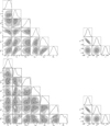Fig. A.1. Method A contour plots from the calibrated Ep–Eiso correlation. Top panels: the best-fit parameters at the dark energy – matter and radiation equivalence. Bottom panels: the best-fit parameters at the dark energy – radiation equivalence. Darker (lighter) areas mark the 1σ (2σ) confidence regions.

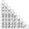Fig. A.2. Method B contour plots, got from the HBR technique, of the best-fit parameters of the Ep–Eiso correlation and the cosmographic approach at the dark energy – matter and radiation equivalence. Darker (lighter) areas mark the 1σ (2σ) confidence regions.

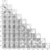Fig. A.3. Method B contour plots, got from the HBR technique, of the best-fit parameters of the Ep–Eiso correlation and the cosmographic approach at the dark energy – radiation equivalence. Darker (lighter) areas mark the 1σ (2σ) confidence regions.

All Tables

All Figures

	Fig. 1. Left: Comparison between the observed Ep, i–Eiso, i sample (Khadka et al. 2021) (gray data) and the simulated Ep, j–Eiso, j sample (green data). Right: Comparison between the distributions of the observed (gray chart) and simulated (green chart) redshifts.
In the text

	Fig. A.1. Method A contour plots from the calibrated Ep–Eiso correlation. Top panels: the best-fit parameters at the dark energy – matter and radiation equivalence. Bottom panels: the best-fit parameters at the dark energy – radiation equivalence. Darker (lighter) areas mark the 1σ (2σ) confidence regions.
In the text

	Fig. A.2. Method B contour plots, got from the HBR technique, of the best-fit parameters of the Ep–Eiso correlation and the cosmographic approach at the dark energy – matter and radiation equivalence. Darker (lighter) areas mark the 1σ (2σ) confidence regions.
In the text

	Fig. A.3. Method B contour plots, got from the HBR technique, of the best-fit parameters of the Ep–Eiso correlation and the cosmographic approach at the dark energy – radiation equivalence. Darker (lighter) areas mark the 1σ (2σ) confidence regions.
In the text

References

- Alfano, A. C., Cafaro, C., Capozziello, S., & Luongo, O. 2023, Phys. Dark Universe, 42, 101298 [NASA ADS] [CrossRef] [Google Scholar]
- Alfano, A. C., Luongo, O., & Muccino, M. 2024a, J. Cosmol. Astropart. Phys., 2024, 055 [Google Scholar]
- Alfano, A. C., Capozziello, S., Luongo, O., & Muccino, M. 2024b, J. High Energy Astrophys., 42, 178 [NASA ADS] [CrossRef] [Google Scholar]
- Alfano, A. C., Luongo, O., & Muccino, M. 2025, J. High Energy Astrophys., 46, 100348 [Google Scholar]
- Amati, L., & Della Valle, M. 2013, Int. J. Mod. Phys. D, 22, 1330028 [NASA ADS] [CrossRef] [Google Scholar]
- Amati, L., Frontera, F., Tavani, M., et al. 2002, A&A, 390, 81 [NASA ADS] [CrossRef] [EDP Sciences] [Google Scholar]
- Amati, L., D’Agostino, R., Luongo, O., Muccino, M., & Tantalo, M. 2019, MNRAS, 486, L46 [CrossRef] [Google Scholar]
- Amati, L., O’Brien, P. T., Götz, D., et al. 2021, Exp. Astron., 52, 183 [NASA ADS] [CrossRef] [Google Scholar]
- Arjona, R., Cardona, W., & Nesseris, S. 2019, Phys. Rev. D, 99, 043516 [NASA ADS] [CrossRef] [Google Scholar]
- Aviles, A., & Cervantes-Cota, J. L. 2011, Phys. Rev. D, 84, 083515; Erratum: Phys. Rev. D, 84, 089905 [Google Scholar]
- Aviles, A., Gruber, C., Luongo, O., & Quevedo, H. 2012, Phys. Rev. D, 86, 123516 [CrossRef] [Google Scholar]
- Aviles, A., Klapp, J., & Luongo, O. 2017, Phys. Dark Univ., 17, 25 [Google Scholar]
- Belfiglio, A., Giambò, R., & Luongo, O. 2023, Classical Quantum Gravity, 40, 105004 [Google Scholar]
- Belfiglio, A., Carloni, Y., & Luongo, O. 2024, Phys. Dark Universe, 44, 101458 [Google Scholar]
- Belfiglio, A., Luongo, O., & Mengoni, T. 2025, Phys. Rev. D, 111, 123512 [Google Scholar]
- Bennett, C. L., Halpern, M., Hinshaw, G., et al. 2003, ApJS, 148, 1 [Google Scholar]
- Bergstrom, L. 2009, New J. Phys., 11, 105006 [CrossRef] [Google Scholar]
- Bridle, S. L., Lahav, O., Ostriker, J. P., & Steinhardt, P. J. 2003, Science, 299, 1532 [Google Scholar]
- Cao, S., Dainotti, M., & Ratra, B. 2022, MNRAS, 512, 439 [NASA ADS] [CrossRef] [Google Scholar]
- Capozziello, S., D’Agostino, R., & Luongo, O. 2019, Int. J. Mod. Phys. D, 28, 1930016 [NASA ADS] [CrossRef] [Google Scholar]
- Capozziello, S., D’Agostino, R., & Luongo, O. 2020, MNRAS, 494, 2576 [NASA ADS] [CrossRef] [Google Scholar]
- Capozziello, S., D’Agostino, R., & Luongo, O. 2022a, Phys. Dark Univ., 36, 101045 [Google Scholar]
- Capozziello, S., Dunsby, P. K. S., & Luongo, O. 2022b, MNRAS, 509, 5399 [Google Scholar]
- Carloni, Y., Luongo, O., & Muccino, M. 2025, Phys. Rev. D, 111, 023512 [Google Scholar]
- Cattoën, C., & Visser, M. 2007, Classical Quantum Gravity, 24, 5985 [Google Scholar]
- Chevallier, M., & Polarski, D. 2001, Int. J. Mod. Phys. D, 10, 213 [Google Scholar]
- Copeland, E. J., Sami, M., & Tsujikawa, S. 2006, Int. J. Mod. Phys. D, 15, 1753 [NASA ADS] [CrossRef] [Google Scholar]
- Cucchiara, A., Levan, A. J., Fox, D. B., et al. 2011, ApJ, 736, 7 [Google Scholar]
- Cuceu, A., Farr, J., Lemos, P., & Font-Ribera, A. 2019, JCAP, 2019, 044 [Google Scholar]
- D’Agostino, R., Luongo, O., & Muccino, M. 2022, Classical Quantum Gravity, 39, 195014 [Google Scholar]
- Dainotti, M. G., Sarracino, G., & Capozziello, S. 2022, PASJ, 74, 1095 [NASA ADS] [CrossRef] [Google Scholar]
- DESI Collaboration (Adame, A. G., et al.) 2025, JCAP, 2025, 021 [Google Scholar]
- Dunsby, P. K. S., & Luongo, O. 2016, Int. J. Geom. Meth. Mod. Phys., 13, 1630002 [NASA ADS] [CrossRef] [Google Scholar]
- Efstathiou, G., & Gratton, S. 2020, MNRAS, 496, L91 [Google Scholar]
- Eisenstein, D. J., Zehavi, I., Hogg, D. W., et al. 2005, ApJ, 633, 560 [Google Scholar]
- Fana Dirirsa, F., Razzaque, S., Piron, F., et al. 2019, ApJ, 887, 13 [Google Scholar]
- Hinshaw, G., Spergel, D. N., Verde, L., et al. 2003, ApJS, 148, 135 [Google Scholar]
- Hu, J.-P., & Wang, F.-Y. 2023, Universe, 9, 94 [CrossRef] [Google Scholar]
- Izzo, L., Luongo, O., & Capozziello, S. 2012, Mem. Soc. Astron. Ital. Suppl., 19, 37 [Google Scholar]
- Jia, X. D., Hu, J. P., Yang, J., Zhang, B. B., & Wang, F. Y. 2022, MNRAS, 516, 2575 [Google Scholar]
- Jimenez, R., & Loeb, A. 2002, ApJ, 573, 37 [NASA ADS] [CrossRef] [Google Scholar]
- Khadka, N., Luongo, O., Muccino, M., & Ratra, B. 2021, JCAP, 2021, 042 [Google Scholar]
- Khetan, N., Izzo, L., Branchesi, M., et al. 2021, A&A, 647, A72 [NASA ADS] [CrossRef] [EDP Sciences] [Google Scholar]
- King, A. L., Davis, T. M., Denney, K. D., Vestergaard, M., & Watson, D. 2014, MNRAS, 441, 3454 [Google Scholar]
- Kodama, Y., Yonetoku, D., Murakami, T., et al. 2008, MNRAS, 391, L1 [NASA ADS] [CrossRef] [Google Scholar]
- Kogut, A., Spergel, D. N., Barnes, C., et al. 2003, ApJS, 148, 161 [NASA ADS] [CrossRef] [Google Scholar]
- Kumar, D., Jain, D., Mahajan, S., Mukherjee, A., & Rana, A. 2023, Int. J. Mod. Phys. D, 32, 2350039 [Google Scholar]
- Li, L.-X. 2007, MNRAS, 379, L55 [Google Scholar]
- Li, M., Li, X.-D., Wang, S., & Wang, Y. 2013, Front. Phys., 8, 828 [Google Scholar]
- Linder, E. V. 2003, Phys. Rev. Lett., 90, 091301 [Google Scholar]
- Lobo, F. S. N., Mimoso, J. P., & Visser, M. 2020, JCAP, 2020, 043 [CrossRef] [Google Scholar]
- Luongo, O. 2025, ArXiv e-prints [arXiv:2504.09987] [Google Scholar]
- Luongo, O., & Muccino, M. 2018, Phys. Rev. D, 98, 103520 [CrossRef] [Google Scholar]
- Luongo, O., & Muccino, M. 2021a, Galaxies, 9, 77 [NASA ADS] [CrossRef] [Google Scholar]
- Luongo, O., & Muccino, M. 2021b, MNRAS, 503, 4581 [NASA ADS] [CrossRef] [Google Scholar]
- Luongo, O., & Muccino, M. 2023, MNRAS, 518, 2247 [Google Scholar]
- Luongo, O., & Muccino, M. 2024, A&A, 690, A40 [NASA ADS] [CrossRef] [EDP Sciences] [Google Scholar]
- Luongo, O., & Quevedo, H. 2014, Phys. Rev. D, 90, 084032 [Google Scholar]
- Luongo, O., Pisani, G. B., & Troisi, A. 2016, Int. J. Mod. Phys. D, 26, 1750015 [Google Scholar]
- Martins, C. J. A. P., & Prat Colomer, M. 2018, A&A, 616, A32 [NASA ADS] [CrossRef] [EDP Sciences] [Google Scholar]
- Melchiorri, A., Pagano, L., & Pandolfi, S. 2007, Phys. Rev. D, 76, 041301 [Google Scholar]
- Montiel, A., Cabrera, J. I., & Hidalgo, J. C. 2021, MNRAS, 501, 3515 [Google Scholar]
- Moresco, M., Jimenez, R., Verde, L., Cimatti, A., & Pozzetti, L. 2020, ApJ, 898, 82 [NASA ADS] [CrossRef] [Google Scholar]
- Moresco, M., Amati, L., Amendola, L., et al. 2022, Living Rev. Relativ., 25, 6 [NASA ADS] [CrossRef] [Google Scholar]
- Muccino, M., Izzo, L., Luongo, O., et al. 2021, ApJ, 908, 181 [Google Scholar]
- Muccino, M., Luongo, O., & Jain, D. 2023, MNRAS, 523, 4938 [NASA ADS] [CrossRef] [Google Scholar]
- Ooba, J., Ratra, B., & Sugiyama, N. 2018, ApJ, 864, 80 [Google Scholar]
- Padmanabhan, T. 2003, Phys. Rep., 380, 235 [Google Scholar]
- Peebles, P. J., & Ratra, B. 2003, Rev. Mod. Phys., 75, 559 [NASA ADS] [CrossRef] [Google Scholar]
- Perivolaropoulos, L., & Skara, F. 2022, New Astron. Rev., 95, 101659 [CrossRef] [Google Scholar]
- Perlmutter, S., Aldering, G., della Valle, M., et al. 1998, Nature, 391, 51 [CrossRef] [Google Scholar]
- Perlmutter, S., Aldering, G., Goldhaber, G., et al. 1999, ApJ, 517, 565 [Google Scholar]
- Planck Collaboration VI. 2020, A&A, 641, A6 [NASA ADS] [CrossRef] [EDP Sciences] [Google Scholar]
- Profumo, S., Giani, L., & Piattella, O. F. 2019, Universe, 5, 213 [Google Scholar]
- Riess, A. G., Filippenko, A. V., Challis, P., et al. 1998, AJ, 116, 1009 [Google Scholar]
- Riess, A. G., Yuan, W., Macri, L. M., et al. 2022, ApJ, 934, L7 [NASA ADS] [CrossRef] [Google Scholar]
- Risaliti, G., & Lusso, E. 2019, Nat. Astron., 3, 272 [Google Scholar]
- Rodney, S. A., Riess, A. G., Scolnic, D. M., et al. 2015, AJ, 150, 156 [NASA ADS] [CrossRef] [Google Scholar]
- Rubano, C., & Scudellaro, P. 2002, ArXiv e-prints [arXiv:astro-ph/0203225] [Google Scholar]
- Sahni, V., & Starobinsky, A. 2000, Int. J. Mod. Phys. D, 9, 373 [Google Scholar]
- Scolnic, D. M., Jones, D. O., Rest, A., et al. 2018, ApJ, 859, 101 [NASA ADS] [CrossRef] [Google Scholar]
- Spergel, D. N., Verde, L., Peiris, H. V., et al. 2003, ApJS, 148, 175 [Google Scholar]
- Tanvir, N. R., Fox, D. B., Levan, A. J., et al. 2009, Nature, 461, 1254 [Google Scholar]
- Tonry, J. L., Schmidt, B. P., Barris, B., et al. 2003, ApJ, 594, 1 [NASA ADS] [CrossRef] [Google Scholar]
- Tsujikawa, S. 2011, in Astrophysics and Space Science Library, eds. S. Matarrese, M. Colpi, V. Gorini, & U. Moschella, 370, 331 [NASA ADS] [CrossRef] [Google Scholar]
- Tucker, R. W., Burton, D. A., & Noble, A. 2005, Gen. Relativ. Gravitation, 37, 1555 [Google Scholar]
- Visser, M. 2005, Gen. Relativ. Gravitation, 37, 1541 [Google Scholar]
- Visser, M., Cattoën, Céline, 2010, in Dark Matter in Astrophysics and Particle Physics, Dark 2009, eds. H. V. Klapdor-Kleingrothaus, & I. V. Krivosheina, 287 [Google Scholar]
- von Marttens, R., Lombriser, L., Kunz, M., et al. 2020, Phys. Dark Univ., 28, 100490 [Google Scholar]
- Wang, J. S., Wang, F. Y., Cheng, K. S., & Dai, Z. G. 2016, A&A, 585, A68 [NASA ADS] [CrossRef] [EDP Sciences] [Google Scholar]