| Issue |
A&A
Volume 700, August 2025
|
|
|---|---|---|
| Article Number | A43 | |
| Number of page(s) | 11 | |
| Section | Atomic, molecular, and nuclear data | |
| DOI | https://doi.org/10.1051/0004-6361/202553949 | |
| Published online | 01 August 2025 | |
X-ray and UV photochemical rates of CO ices
Aix Marseille Univ, CNRS, CINaM,
Marseille,
France
★ Corresponding authors: This email address is being protected from spambots. You need JavaScript enabled to view it.
; This email address is being protected from spambots. You need JavaScript enabled to view it.
Received:
29
January
2025
Accepted:
8
June
2025
Abstract
Context. Compared to UV radiation, X-rays contribute only minimally to the interstellar radiation field, but galactic and stellar objects can produce significant local X-ray fluxes that can impact the chemical composition of nearby gases and icy dust.
Aims. The aim of this study is to provide astrochemists with laboratory data on the X-ray and UV photochemical rates of CO ice, one of the most abundant ices in the universe.
Methods. We used two laboratory sources emitting X-rays (Al Kα, 1486.6 eV) and UV (Lyman-α, 10.2 eV) to measure and compare X-ray and UV photochemical rates of CO ices. We used infrared spectroscopy to probe photodesorption and photodissociation, the two processes being differentiated by covering the CO ice with an argon layer to block photodesorption.
Results. For CO ice at 10 K, we find UV photodesorption rates in line with the existing literature. At 1486.6 eV, X-ray photodesorption rates are an order of magnitude higher than with UV. We show that the X-ray absorption cross section of CO allows astrochemists to scale these X-ray photodesorption rates to the X-ray spectrum of the region of interest. Regarding the CO photodissociation, our measured X-ray rates are two orders of magnitude higher than with UV, and are also proportional to the X-ray absorption cross section. The reformation reaction balances the X-ray destruction of CO, leading to a stable state where only 25% of the initial amount of CO is destroyed, strongly limiting the destruction of CO by X-rays. When this steady state is reached, only X-ray and UV photodesorption need be considered.
Conclusions. This study provides the data needed to model X-ray and UV photochemical processes in CO ices.
Key words: astrochemistry / radiation mechanisms: non-thermal / solid state: volatile / methods: laboratory: solid state / ultraviolet: general / X-rays: general
© The Authors 2025
 Open Access article, published by EDP Sciences, under the terms of the Creative Commons Attribution License (https://creativecommons.org/licenses/by/4.0), which permits unrestricted use, distribution, and reproduction in any medium, provided the original work is properly cited.
This article is published in open access under the Subscribe to Open model. This email address is being protected from spambots. You need JavaScript enabled to view it. to support open access publication.
1 Introduction
The interstellar medium is permeated with electromagnetic radiation that influence the physical and chemical properties of gas and icy dust. Interstellar radiation consists mainly of photons with energies below the hydrogen Lyman-α UV radiation (121.6 nm; 10.2 eV). In comparison, the harder X-ray radiation is six to ten orders of magnitude less intense (Tielens 2005). However, strong X-ray fields can be locally produced by a variety of astrophysical objects, from galaxy clusters to stars, such as X-ray binaries, super soft X-ray sources, or T Tauri stars. Of these sources, the latter are of particular interest for understanding the formation of planets in their protoplanetary disks. T Tauri stars emit an intense X-ray flux in the 0.1-10 keV range (Walsh et al. 2012) that can penetrate their circumstellar environments much more effectively than UV radiation (Notsu et al. 2021; Walsh et al. 2012); disk matter is also exposed to external and background UV and X-ray radiation fields (Walsh et al. 2013; Rab et al. 2018; Ciesla & Sandford 2012) and all these radiations affect the composition of gas and icy dust of pro-toplanetary disks, where CO ices are a significant component of the peripheral regions (Arabhavi et al. 2024; Bruderer et al. 2009; Van Dishoeck 2006; Stäuber et al. 2007; Walsh et al. 2010, 2012, 2015; Boogert et al. 2015).
For decades, numerous laboratory experiments on the photochemistry of interstellar ice analogs have focused on UV light, providing essential data such as photodissociation and photodesorption rates and reaction pathways to form complex molecules from simple ones (Öberg 2016). This focus on UV photochemistry has been facilitated by affordable and powerful UV laboratory sources such as microwave discharge hydrogen flow lamps (Chen et al. 2014). In contrast, X-ray laboratory experiments on ices are rare and even fewer studies compare the effects of X-ray and UV radiation. One reason is that X-ray sources are rarely available on laboratory astrochemistry experiments, and most existing X-ray studies are conducted using synchrotron radiation, whose access is severely time-limited. Pioneering synchrotron work by Parent et al. two decades ago used X-ray absorption spectroscopy (NEXAFS) to study the soft X-ray (100-1500 eV) photochemistry of various ices, including H2O (Laffon et al. 2006), O2:H2O (Lacombe et al. 2006), ammonia NH3 (Parent et al. 2009), CO and methanol CH3OH (Laffon et al. 2010), and H2O:glycine ices (Pernet et al. 2013), also investigated by Tzvetkov & Netzer (2011). Later, Ciaravella et al. conducted a series of synchrotron experiments combining soft X-ray irradiation and infrared (IR) spectroscopy on increasingly complex ices, from CO (Ciaravella et al. 2012, 2016), CH3OH (Chen et al. 2013), CO:H2O (Jiménez-Escobar et al. 2016), and H2O:NH3 (Jiménez-Escobar et al. 2018), to H2O:CO:NH3 (Ciaravella et al. 2019) and H2O:CH4:NH3:CO:CH3OH (Ciaravella et al. 2020). They also reviewed several X-ray and UV photochemical studies on CO, H2O:CO and H2O:CO:NH3 (Munõz Caro et al. 2019), showing that both X-ray and UV excitations produce similar byproducts. This is due to the fact that secondary electrons from the nonradiative decay of X-ray excitations (the Auger effect) deplete the molecular valence shells in a manner similar to ionizing UV excitations, leading to a similar radical chemistry (Laffon et al. 2006). Pilling et al. have conducted further experiments combining soft X-ray irradiation and IR spectroscopy on various ices, such as H2O:CO2:NH3:SO2 (Pilling & Bergantini 2015), SO2 (De Souza Bonfim et al. 2017), methyl formate and acetic acid C2H4O2 (Rachid et al. 2017), N2:CH4 (Vasconcelos et al. 2017), H2O:CO2:CH4:NH3 (Pilling et al. 2019), methanol CH3OH (Freitas & Pilling 2020), acetone CH3COCH3 (Carvalho & Pilling 2020a), acetonitrile CH3CN (Carvalho & Pilling 2020b), hydrogen peroxide H2O2 (Pilling & Freitas 2023) and ethanol CH3CH2OH (Pilling & da Silva 2023). Using photon-stimulated desorption NEXAFS spectroscopy (PSD-NEXAFS), Fillion and co-workers studied and quantified X-ray-induced photodesorption of ices of H2O (Dupuy et al. 2018, 2020), methanol CH3OH (Basalgète et al. 2021a), CH3OH:CO and CH3OH:H2O (Basalgète et al. 2021b), CO (Dupuy et al. 2021), N2:CO (Basalgète et al. 2022), and acetonitrile CH3CN (Basalgète et al. 2023). Finally, recent studies have investigated the role of carbon grains in the energetic irradiation of water ice deposited on their surface, with UV (Potapov et al. 2023) and X-rays (Chuang et al. 2023).
Infrared spectroscopy is widely used to study how laboratory ices evolve under irradiation. By tracking the decrease in intensity of an IR absorption band over the irradiation time, one can determine the rates of photochemical processes and evaluate the stability of a molecule in solid form when it is exposed to space radiation. It also tells us about the role of photodesorption in gasgrain exchanges. The appearance of new bands during irradiation also reveals the formation of byproducts and helps estimate their production rates. However, these seemingly simple experiments are not without challenges. Regarding UV irradiation, significant inaccuracies have been well documented to be caused by experimental bias, particularly in estimating the flux and spectral energy distribution of the UV irradiation source (Ligterink et al. 2015). In addition, it is difficult to distinguish between the various competing processes in irradiated ice (Bulak et al. 2023), such as desorption, dissociation, and structural changes (compaction and amorphization), which all impact the IR intensities of CO. This has resulted in significant discrepancies between different studies, sometimes of several orders of magnitude for measurements as simple as the UV desorption rate of CO ice (Paardekooper et al. 2016). Regarding X-ray studies, experiments using synchrotron radiation also face a number of challenges. One significant issue is the overlap between the area irradiated by the X-ray focused beam and the area probed by the larger IR beam (Chen et al. 2013; Jiménez-Escobar et al. 2016); this does not concern synchrotron experiments, where desorption rates are measured with a mass spectrometer or where byproducts are characterized with a synchrotron technique such as NEXAFS spectroscopy, since the zone probed is also the irradiated zone. To resolve this overlap issue, one has to accurately estimate the ratio of the IR to X-ray beam sizes for a proper quantification of the photochemical rates, which is a difficult task. In the present work, we present a new laboratory setup equipped with a powerful X-ray source delivering a beam of large size combined with IR spectroscopy. It solves at the same time the problem of access time and beam overlap, and is ideal for quantitative X-ray measurement experiments. Furthermore, the addition of a UV source that illuminates the sample at the same point as the X-rays enables a reliable comparison between the effects of the two radiations.
The few previous studies using laboratory X-ray tubes with a carbon anode to investigate the X-ray photolysis of CH3OH (Ciaravella et al. 2010) and CO (Ciaravella et al. 2012) ices were limited by the low efficiency of carbon’s Kα emission line at 277 eV (Krause 1979). This anode delivers a weak flux and is not capable of exciting the 1s electrons of carbon, nitrogen, and oxygen, making it hardly suitable for studying the photochemistry of organic molecules, or molecules such as H2O or NH3. For the present study, we use the intense Kα emission from an aluminum anode at 1486.6 eV, which closely matches the energy maximum of the radiation of T Tauri star (Walsh et al. 2012). These X-ray tubes are commercially available, affordable, and commonly used in X-ray photoelectron spectroscopy (XPS) experiments.
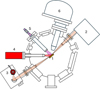 |
Fig. 1 SUMO analysis chamber. (1) Sample position; (2) FTIR spectrometer; (3) FTIR’s MCT detector; (4) X-ray source; (5) UV source; (6) Hemispherical electron analyzer for XPS experiments. |
2 Methods
This article is the first report of our metrological analysis of the UV and X-ray photochemical rates on ice layers. Here we detail the most important aspects of the experimental procedure. Figure 1 shows the analysis chamber of the SUMO ultra-high vacuum (UHV) setup used for this study. It integrates a UV and an X-ray source. The ice layers are deposited onto a 25 × 25 mm gold foil (99.99% purity, Alfa Aesar) in an upper UHV chamber (not shown), which is isolated from the analysis chamber by a gate valve to prevent contamination. Before each experiment, the gold foil is cleaned at room temperature with a 4 keV argon ion beam. The gold foil is mounted on the cold finger of a cryostat cooled by a closed-cycle cryogenerator (SHI Cryogenics DE204B) to maintain the temperature at a minimum of 10±1 K. The sample temperature is measured with a silicon diode clamped near the sample (Lakeshore DT670), and heating can be achieved using a PID-controlled 50 W heater. The upper chamber is equipped with several independent leak valves for multiple gas exposures; two Bayard-Alpert ion gauges and a mass spectrometer (Hiden Hal200) allow the molecular fluxes to be monitored.
After deposition of the ice film in the upper chamber, we transfer the sample to the sample position of the analysis chamber (labeled 1 in Fig. 1) for reflection-absorption IR spectroscopy (RAIRS), carried out at a grazing angle of 6±2° with a Fourier transform IR (FTIR) spectrometer (Jasco 6300V, labeled 2 in Fig. 1). The IR optical path outside the analysis chamber is kept under primary vacuum to prevent contamination from atmospheric CO2 and H2O. A mercury-cadmium-telluride (MCT) detector (labeled 3 in Fig. 1) is used to collect the IR signal. It is housed in a vacuum chamber and its liquid nitrogen Dewar is equipped with an extension (Kadel) allowing up to several days of continuous experiments without needing to refill, which enables us to perform long irradiation studies. The MCT detector is connected to a turbo molecular pump (Pfeiffer HiPace 300) maintaining a dynamic secondary vacuum inside the detector’s Dewar. This ensures that during long experiments, the IR signal is not contaminated by the slow condensation of H2O and CO2 ices on the MCT surface. To measure the photoreaction rates, we monitor the decrease in intensity of the infrared absorption bands of the CO molecule (2142-2138 cm−1) during irradiation. It is therefore crucial to understand the relationship between the IR intensity and the column density (or thickness) of the molecular layer, which is known to be nonlinear in RAIRS. This point is explored in detail in Appendix A.
The X-ray source (PSP Vacuum TX400, labeled 4 in Fig. 1) is positioned at a 45° angle to the sample surface’s normal. It features a magnesium anode (Mg Kα, 1253.6 eV) and an aluminum anode (Al Kα, 1486.6 eV), mainly used in this work. It is cooled by a closed-circuit water chiller and operates at a maximum power of 300 W for Mg and 400 W for Al. A hemispherical electron analyzer (PSP Resolve 120, labeled 6 in Fig. 1) is used for complementary XPS measurements. Calibration with a fluorescent screen confirms that the X-ray beam covers the entire surface of the sample. This is important because the IR beam spreads across the entire sample surface, due to its grazing angle of incidence; the broad size of the X-ray beam guarantees that the area probed by the IR has been irradiated by X-rays. We note that this perfect overlap between the X-ray and IR beams is lost if a monochromatized laboratory X-ray source producing a submillimeter focused beam is used, generating overlap problems as with synchrotron radiation. Furthermore, the infrared RAIRS configuration ensures that only the molecules deposited on the substrate and X-ray irradiated are probed by the IR beam. By contrast, in an infrared transmission geometry, molecules deposited on both sides of the transparent IR window contribute to the infrared signal, but as the X-ray beam is not transmitted through this window, only one side is irradiated and measuring the X-ray photolysis rate is difficult.
The UV source is a microwave-discharge hydrogen lamp (MDHL) (Opthos, labeled 5 in Fig. 1). This lamp emits hydrogen Lyman-α radiation mimicking the interstellar UV field. It is a sealed glass tube with a MgF2 window at one end, filled with a gas mixture of 10% H2 and 90% argon at a pressure of 1 Torr. An Evenson cavity provides microwave excitation at 2450 MHz with a maximum power of 100 W. The light emitted by the lamp is transmitted inside the SUMO analysis chamber through a viewport also equipped with a MgF2 window and is then guided through an aluminum tube to the sample surface.
The flux delivered by both the UV and X-ray sources is calibrated with a photodiode sensitive to UV and X-ray (XUV100C, UDT Sensors) positioned as the sample would be. For UV calibration, the light passing through a quartz window (visible light only) is subtracted from the total flux (visible light + UV), which we found consists of 90% visible light and 10% UV light. The photodiode cannot be used during irradiation experiments as the sample must be positioned in its place. To read the UV flux during irradiations, an electrically insulated copper mesh with 90% transmittance is affixed to the end of the aluminum light guide, providing a photocurrent that has been previously scaled against the photodiode. This photocurrent is continuously recorded using a picoammeter (Keithley Model 617), enabling us to correct for any UV flux variations. Unlike the MDHL, the flux of the X-ray source is stable during irradiation, so realtime monitoring is unnecessary. X-ray irradiations are carried out with a typical power of 350 W for Al Kα and 270 W for Mg Kα, corresponding to X-ray fluxes of 1 × 10¹³ and 6 × 10¹² ph cm−2 s−1, respectively. These fluxes are four orders of magnitude higher than those measured with a laboratory X-ray carbon source (Ciaravella et al. 2012) and are comparable to synchrotron radiation fluxes used in previous X-ray studies, ranging from 5 × 10¹⁰ ph cm−2 s−1 (Chen et al. 2013) to 1 × 10¹⁴ ph cm−2 s−1 (Carvalho & Pilling 2020a). UV irradiations are carried out with a power of 80 W (reflecting power <5 W), corresponding to UV fluxes of 4 × 10¹³ ph cm−2 s−1. The irradiation times are around 20 h for X-rays and 5 h for UV (similar results are obtained for 20 h irradiations with lower UV flux), resulting in a fluence (or cumulated dose) in the range of 7 × 10¹⁷ ph cm−2 s−1.
The systems studied comprise CO ices deposited at 10 K with molecular thicknesses up to 8 monolayers (ML; 1 ML= 1 × 10¹⁵ molec cm−2) to keep the IR signal linear, as explained in Appendix A. The number of molecular layers of CO is calculated from the integrated intensity of the 12CO vibration bands at 2142 and 2138 cm−1 (see Appendix A). The CO layers are deposited either on the bare gold foil or on the gold foil pre-covered with 20 ML of argon. This argon layer serves as a model for an insulating substrate to see whether the metal substrate influences or not the photoprocesses (Menzel 2008).
To distinguish between photodesorption and photodissociation we also add a 16 ML argon buffer layer on top of the CO layers (Bulak et al. 2020). Excited CO molecules formed after photoexcitation have an extremely short trajectory within the ice layer and only those located near the surface can escape in vacuum (Parent & Laffon 2005). These desorbing molecules make the ice thinner, inducing a decrease in intensity of the CO band in a way similar to photodissociation. An argon cap blocks the desorption of CO in the vacuum (Bulak et al. 2020; Gerakines et al. 1996; Loeffler et al. 2005; Öberg et al. 2009), and therefore argon-coated CO layers are devoid of photodesorption while bare CO layers are subject to both photodesorption and photodissociation. By comparing the two cases, we can distinguish between the two processes. We note that the argon buffer undergoes depletion because of X-ray photodesorption. This results in a 7% intensity drop in the argon 2p emission line measured with XPS, corresponding to a loss of approximately 4 ML for the entire dose received. Table 1 summarizes the composition of the studied ices. The relative error on photodesorption and photodissociation rates given in this article is estimated at a rounded value of 30%, as commonly found in similar studies (Paardekooper et al. 2016). This relative error results from the quadratic addition of flux measurement errors, i.e., on the order of 10% for the precision of the calibration diode, 10% for flux variations from the X-ray source and the UV source, and 20% for illumination variations due to the positioning of the sample with respect to the sources. Added to this is a relative error of 10% on the intensity of the infrared bands (integration errors and adjustment errors of the fits).
Summary of the irradiation experiments; numbers are in units of ML.
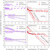 |
Fig. 2 Evolution of the CO column densities (from integrated intensity of the 12CO IR band at 2142 and 2138 cm−1) plotted against exposure to UV and X-rays. (a) UV irradiation of CO:Au and Ar:CO:Au ; (b) UV irradiation of CO:Ar and Ar:CO:Ar; (c) X-ray irradiation of CO:Au and Ar:CO:Au ; (d) X-ray irradiation of CO:Ar and Ar:CO:Ar ; at the equilibrium [CO]eq = α[CO]t=0. |
3 Results
Figure 2 shows the evolution of the column densities of CO on gold and argon substrates during UV irradiation (Figs. 2a and 2b, respectively) and X-ray irradiation (Figs. 2c and 2d, respectively). The labels “dissociation” and “dissociation & desorption” refer to experiments with and without the argon overlayer, as explained previously. In the case of UV irradiation, CO dissociation is negligible and only desorption is observed, hence the simple label “desorption” (Fig. 2, left panel).
3.1 UV irradiations
Figures 2a and 2b show the UV irradiation of approximately 3 and 7 ML of CO deposited on gold (Fig. 2a) and deposited on argon (Fig. 2b). Without the argon cap, the molecular thickness of CO decreases linearly as a result of desorption (open circles). This is a zeroth-order process (Westley et al. 1995; Öberg et al. 2009) and the experimental curves can be fitted by a straight line using Eq. (1):
![Mathematical equation: \rm [CO]_t=[CO]_{t=0}-\sigma\phi t .](/articles/aa/full_html/2025/08/aa53949-25/aa53949-25-eq1.png) (1)
(1)
Here [CO]t=0 and [CO]t are the initial and instantaneous column densities, respectively; σ is the desorption rate, φ is the photon flux, and t is the irradiation time (φt is the fluence). The desorption rates deduced from the linear fits are listed in Table 2. For easier comparison with the literature, these rates are also given in cm2 ph−1 (Cottin et al. 2003; Gerakines et al. 1996). The UV desorption is not significantly influenced by the thickness of the CO layer or the nature of the substrate, whether it is metallic (gold) or insulating (argon).
With the argon cap, the CO column density (filled circles) seems stable, and this is why the UV dissociation of CO is generally deemed negligible; in fact, it imperceptibly decreases. Assuming that the experimental curves can be approximated with a straight line, we can extract faint linear dissociation rates, also listed in Table 2. They are in line with a previous study (Gerakines et al. 1996) that reported <0.8 × 10⁻¹⁹ cm2 ph−1. The low efficiency of the UV dissociation of CO implies that the concentration of photoproducts is low. Our FTIR data (not presented) indicate that few CO2 molecules are primarily formed (≈1% of the initial CO concentration), likely through the Boudouard reaction, where CO reacts with an excited CO* molecule to form CO2 (Laffon et al. 2010):
 (2)
(2)
The other byproducts C3O and C3O2 (Gerakines et al. 1996; Gerakines & Moore 2001) are detected in small amounts with respect to CO2. Despite their significant IR band intensities (Jamieson et al. 2006), other expected byproducts such as C5O2 or C7O2 (Loeffler et al. 2005) remain below our detection limit on these thin layers.
UV desorption and dissociation rates at 10 K. The relative error is estimated at 30%.
3.2 X-ray irradiations
Figs. 2c and 2d show the X-ray (1486.6 eV) irradiation results for CO deposited on gold (approximately 6 ML of CO; for clarity, the 2.8 CO:Au experiment is not presented, but the corresponding rates are listed in Table 3) and for CO deposited on 20 ML of argon (approximately 8 ML of CO).
With the argon cap (filled circles), the decrease in the column density of CO is due to X-ray dissociation only, which is now non-negligible. This decrease starts steeply with an exponential decay slope and then reaches a steady state at a value of [CO]eq. This slope is typical of a first-order reaction where a destruction reaction is balanced by a reformation reaction (Gerakines et al. 2012; Laffon et al. 2010):
 (3)
(3)
The corresponding kinetic equation is (Gerakines et al. 2012; Laffon et al. 2010; Laidler 1987):
![Mathematical equation: \rm [CO]_t=[CO]_{t=0} [(1-\alpha)e^{-\sigma\phi t} + \alpha],](/articles/aa/full_html/2025/08/aa53949-25/aa53949-25-eq4.png) (4)
(4)
where α = [CO]eq/[CO]t=0 is the equilibrium constant and σ is the sum of the destruction and the reformation rates. The experimental curves are well fitted with Eq. (4) (dashed lines), which provides both σ and α (listed in Table 3). Unlike a zero-order process, the dissociation of CO cannot be described solely by a reaction rate σ, because α is a crucial parameter that must be considered. If α =1, the reverse reactions fully balance the forward reactions and the amount of CO will remain at its initial value [CO]t=0, even if the dissociation rate is high. In contrast, if α=0 there is no reverse reaction and all molecules are destroyed. We note that within the argon buffer, the Auger and secondary electrons created after the X-ray photoexcitation of argon might induce dissociation of the CO molecules in the CO layers beneath. It is difficult to estimate the contribution of this effect to the measured rates. If any, it can be likened to an increase in the incident photon flux, which will lead to an apparent increase in the X-ray photodissociation yields listed in Table 3. These values will appear higher than they would be without the argon buffer and are therefore cautiously indicated as upper values.
Without the argon cap (open circles), the decrease in the column density of CO is due to dissociation and desorption. This decrease starts linearly and asymptotically tends to the disappearance of the CO layer. Desorption alone can be estimated by subtracting from these curves those obtained with the argon cap (dissociation alone). This difference gives the black curves (dashed lines) labeled “desorption (estimated)”. After about 1 × 10¹⁷ ph cm−2 the dissociation curve becomes constant and the difference curve becomes linear, indicating a zeroth-order process, as in UV. Therefore, the constant negative slopes of the linear part of these difference curves are fitted with Eq. (1), providing the X-ray desorption rates given in Table 3. At the energy of 1486.6 eV, X-ray desorption rates are typically an order of magnitude higher than those measured with UV (Table 2). However, as discussed below, these X-ray desorption rates highly depend on the irradiation energy.
To keep the article concise, the IR spectra of the X-ray byproducts are not presented here, but are briefly discussed. We observe CO2 and polycarbon CnO species (C2O, C3O, C4O, C6O) and CmO2 species (C3O2 and C5O2), similar to those reported in previous X-ray studies (Ciaravella et al. 2016), and with higher concentrations than in our UV irradiations due to the higher X-ray destruction rates. These species are also observed in UV on thick ices in transmission (Gerakines et al. 1996; Gerakines & Moore 2001; Loeffler et al. 2005), and with ion (Loeffler et al. 2005; Palumbo et al. 2008) and electron irradiations (Jamieson et al. 2006; Huang et al. 2020). The analysis of the IR data on the argon-capped layers shows that the concentration of CO2 increases exponentially and saturates at an equilibrium value [CO2]eq when CO reaches its equilibrium concentration [CO]eq. The column density of CO2 can be derived from the integrated intensity of the ν3 asymmetric stretching mode at 2348 cm−1 with a band strength of 1.4 × 10⁻¹⁶ cm molec−1 (Hudgins et al. 1993). The ratio of [CO2]eq to [CO]eq is about 5% (Table 3). The CO2 concentrations are also higher than with UV because other channels such as CO + O add to the Boudouard reaction to form CO2.
In the case of UV, the substrate does not play a major role in photodesorption (or dissociation) as the rates measured for gold and argon are very similar. In the case of X-rays, the situation may be different because of the electron flow stemming from the X-ray excitation of the substrate. However, unraveling the mechanisms underlying photodesorption requires dedicated experiments and is well beyond the scope of this work. Existing studies indicate that photodesorption of molecularly adsorbed CO on metal surfaces predominantly proceeds through direct photoexcitation of the adsorbed molecules themselves (Franchy & Menzel 1979). In these scenarios, photoinduced electrons generated within the metal substrate appear to play only a minor role, even when CO binds strongly to the surface (Frigo et al. 1998). As a result, the substrate exerts minimal influence on the overall desorption rate. Nevertheless, indirect desorption mechanisms have also been proposed, including those involving secondary and Auger electrons produced by X-ray excitation of the substrate. These electrons can contribute to the desorption of surface molecules via a process known as X-ray-induced electron-stimulated desorption (XESD). On ices the relevance of XESD has been experimentally demonstrated in systems such as CO adsorbed on N2 ice (Basalgète et al. 2022). Because the number of electrons generated under X-ray irradiation depends on the atomic properties of the substrate, materials such as argon, being lighter than gold and possessing a lower X-ray absorption cross section, produce fewer secondary electrons. Consequently, XESD in argon is expected to be less efficient than in gold. This discrepancy might explain the observed difference in X-ray photodesorption yields between the two substrates (1.4 × 10⁻² molec ph−1 for argon vs. 2.3 × 10⁻² molec ph−1 for gold), although the variation falls within the range of experimental uncertainty. To conclusively determine the influence of substrate composition on X-ray photodesorption of CO, further studies are essential, particularly those involving more astrophys-ically relevant materials, such as silicates or analogs of cosmic dust grains, with and without icy coatings.
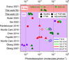 |
Fig. 3 CO desorption rates: X-rays (top area, red) and UV (bottom area, magenta), updated from the review of Paardekooper et al. (2016), with the addition of our UV and X-ray (1486.6 eV) data, and the X-ray data of Dupuy et al. (2021) taken at 600 eV and scaled at 1486.6 eV (see text). The experimental methods are indicated by the shape of the points: LD TOF-MS is for laser desorption time-of-flight mass spectrometry; NEX-AFS/MS is for NEXAFS spectroscopy coupled with Mass Spectrometry (PSD-NEXAFS). |
4 Discussion
4.1 Photodesorption
4.1.1 UV photodesorption
Figure 3 compares our UV photodesorption rates (green triangles) with those from previous works. This figure was derived and updated from the review of Paardekooper et al. (2016). It illustrates how different the UV desorption rates of CO are in the literature. As mentioned above, this can result from differences in the spectral characteristics of the UV sources used since desorption strongly varies in the 8-11 eV range (Fayolle et al. 2011). Other factors can affect the UV desorption rate, such as issues with the calibration of the UV flux or the aging of MgF2 windows that separate the UV source from the vacuum experiment where the ices are deposited (Paardekooper et al. 2016; Sie et al. 2022). Intrinsic parameters also influence the UV desorption rates. For instance, the UV desorption yield decreases with the temperature of the ice film (Öberg et al. 2009; Sie et al. 2022).
The film thickness has not been reported to have an effect on the desorption yield of 2-300 ML (Öberg et al. 2007), which is consistent with the fact that photodesorption is limited to the surface layers. This observation was later contradicted by Sie et al. (2022) who found a strong decrease for CO films with thickness values smaller than 30 ML. In our case, we do not observe significant differences in the UV rates with thickness (between 2 and 8 ML), in agreement with Öberg et al. (2007). Our UV rates are also in agreement with those reported by Öberg et al. (2007, 2009), who used a similar combination of RAIRS and MDHL sources and the same thickness range.
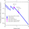 |
Fig. 4 Experimental desorption rates. This work: CO:Ar (blue triangles) at 1486.6 eV (Al Ka) and 1253.6 eV (Mg Ka); Dupuy et al. (2021): Measured at 600 eV (pink star), scaled at 1253.6 eV (pink triangle), scaled at 1486.6 eV (pink circle). Extrapolated rates from the CO X-ray absorption cross section (NIST) (dotted lines) scaled using the desorption rates of CO:Ar at 1486.6 eV (Al Ka). The stripe indicates the margin of error in the NIST data. |
4.1.2 X-ray photodesorption
Our X-ray desorption rates are also reported in the upper part of Fig. 3 (green triangles). They are compared with the data of Dupuy et al. (2021) who measured 0.15 molec ph−1 at 600 eV. As for the UV range (Fayolle et al. 2011), the X-ray photodesorption yield is proportional to the absorption cross section (Parent et al. 2002; Dupuy et al. 2018, 2020, 2021). We can then compare the data obtained at 600 and at 1486.6 eV by accounting for the relative X-ray interaction efficiency between the two energies. For this purpose, we use the X-ray linear attenuation coefficient from the NIST Standard Reference Database 66 (FFAST)1 (Chantler 1995). In the soft X-ray energy range (0.1-10 keV), the attenuation coefficient consists essentially of the photoelectric effect (X-ray absorption), the X-ray scattering being negligible. For CO, the calculated X-ray linear attenuation coefficient μ at 600 eV is 9977 and 912 cm−1 at 1486.6 eV (using a density of 0.8 g cm−3). The absorption efficiency ratio is given by μ(600 eV)/g(1486.6 eV) = 9977/912= 10.9. This makes 0.15 molec ph−1 measured at 600 eV equivalent to 0.15/10.9 = 0.014 molec ph−1 at 1486.6 eV (green star in the upper part of Fig. 3), in perfect agreement with our results.
This proportionality of the photodesorption rates to the X-ray absorption cross section is further illustrated in Figure 4. This figure shows the X-ray linear attenuation coefficient of CO between 0.1 and 10 keV from the NIST database, scaled to match our photodesorption rate obtained at 1486.6 eV on CO deposited on argon (filled blue triangle). The discontinuities in the absorption signal are the carbon K-edge (around 300 eV) and the oxygen K-edge (around 530 eV). Because the X-ray photochemical rate is proportional to the X-ray absorption cross section, the higher the energy, the less efficient the photochemical process (except around absorption thresholds).
We also added in Fig. 4 the photodesorption rate at 1253.6 eV (Mg Kα), which we measured as equal to 2.3 × 10⁻² molec ph−1 (empty blue triangle) on a 7 ML of CO deposited on argon. It is 1.53 times higher than at 1486.6 eV (1.5 × 10⁻² molec ph−1; filled blue triangle), which is in excellent agreement with the predicted value of 1.6 from the NIST database, where μ(1253.6 eV)/μ(1486.6 eV)= 1.6. We have also reported the X-ray desorption rate measured by Dupuy et al. (2021) at 600 eV (pink star) which is scaled at 1253.6 eV using the ratio of X-ray attenuation coefficients μ(600 eV)/μ(1253.6 eV) = 6.8 (empty pink triangle) and at 1486.6 eV using the ratio μ(600 eV)/μ(1486.6 eV) = 10.9 (empty pink circle). The data scaled are also in excellent agreement with our experimental data at 1253.6 and 1486.6‘eV, validating the fact that the desorption rate is proportional to the X-ray attenuation coefficient.
4.2 Photodissociation
4.2.1 UV photodissociation
As said previously, UV dissociation of CO is considered in general negligible, and therefore rate values in UV studies are not given, with the exception of Gerakines et al. (1996) who reported UV dissociation rates <0.8 × 10⁻¹⁹ cm2 ph−1, in good agreement with our values (0.9-2 × 10⁻¹⁹ cm2 ph−1). The production rates of CO2 relative to the initial CO concentration are sometimes quoted (e.g., 0.8% (Gerakines et al. 1996), 1.8% (Loeffler et al. 2005), or 3.5% (Bulak et al. 2020). The low concentrations observed in this work (≈1%) also agree with the 0.8% reported by Gerakines et al. (1996), who measured similar dissociation rates.
4.2.2 X-ray photodissociation
X-ray dissociation of CO has never been quantified and it is impossible to compare our results with those in the literature. However, the X-ray dissociation rates of some other molecules of astrophysical interest have been measured and reviewed by Carvalho & Pilling (2020a), either in the condensed or gas phases. They reported rate values ranging from 1.5 × 10⁻¹⁷ cm2 ph−1 in the case of acetone ice exposed to white beam irradiation (6 eV-2 keV), down to 1 × 10⁻¹⁸ cm2 ph−1 in the case of formic acid gas exposed to monochromatic irradiation at 290 eV. However, as with UV desorption, there are considerable variations in these rates, depending on the technique and irradiation method used. For example, the same authors reported X-ray dissociation rates for acetone ice ranging from 2 × 10⁻¹⁸ cm2 ph−1 to 1.5 × 10⁻¹⁷ cm2 ph−1 (Carvalho & Pilling 2020a). For the present work we measured a dissociation rate of 1.5 × 10⁻¹⁷ cm2 ph−1, which is in the upper range of the X-ray photochemical rates for the molecules reviewed by Carvalho & Pilling (2020a). As for photodesorption, the dissociation yield might also be proportional to the X-ray absorption cross section. To support this hypothesis, we carried out an additional experiment to measure the dissociation rate at 1253.6 eV (Mg Kα) of a 5.5 ML CO:Au ice film covered with argon. We found a dissociation rate of 2.2 × 10⁻¹⁷ cm2 ph−1, which is 1.5 times the value measured at 1486.6 eV (Table 3), close to the expected ratio μ(1253.6 eV)/μ(1486.6 eV)= 1.6 between the two energies.
X-ray photolysis studies have also constantly reported that after a certain time of irradiation an equilibrium is reached and the composition of the ice no longer changes (Carvalho & Pilling 2021). This steady state is a consequence of the reformation reaction. Our study confirms this effect; an equilibrium is reached when about 25% of the CO molecules have been destroyed (α=0.75). This is higher than the 7-10% previously obtained using white-beam synchrotron irradiation (250-1200 eV) of CO at 14 K (Ciaravella et al. 2016). In contrast, it is lower than in our previous study carried out at 20 K with synchrotron white beam irradiation (1-1000 eV) (Laffon et al. 2010) where 40% of the CO was lost, but dissociation and desorption were measured simultaneously. In these works the measurement method, the irradiation energy values, and the ice temperature were not identical, making comparisons difficult. The dissociation values measured at a given energy cannot be compared with those using white-beam irradiation without integration over the whole energy range used for irradiation. In addition, a higher irradiation temperature increases the thermal diffusion of the initial C and O radicals, reducing the yield of the reverse reaction of (3) and favoring the formation of CO + O → CO2, CO + C → C2O and the subsequent reactions leading to polycarbon species. This increases the net destruction of CO and the formation of CO2, C2O, and CnO species.
5 Astrophysical implications
The astrophysical implications are straightforward: in regions of high UV and X-ray radiation, desorption and dissociation rates are needed to estimate both CO ice abundances and nonthermal transfer of CO from the condensed phase to the gas phase. With such photochemical rates measured in the case of H2O ice (Dupuy et al. 2018), it is possible to model the X-ray induced chemistry of water in protostellar envelopes (Notsu et al. 2021), and the same approach can be pursued in the case of CO.
The photochemical evolution of CO ices results from the addition of desorption and dissociation processes, which remove amounts of CO relative to the original quantity [CO]t=0. UV and X-ray photodesorption of CO are two linear processes (Eq. (1)) that add up. The time evolution of the total photodesorption process can be modeled as
![Mathematical equation: \rm [CO]_{t}^{desorption}=[CO]_{t=0}-\sigma_{desorption}^{UV}\phi_{UV} t -\sigma_{desorption}^{RX}\phi_{RX} t .](/articles/aa/full_html/2025/08/aa53949-25/aa53949-25-eq5.png) (5)
(5)
The UV desorption rates  are those measured with UV at 10.2 eV (Table 2), while the X-ray desorption rates
  relevant to the local X-ray spectrum of the considered region can be obtained with the X-ray absorption cross section scaled to our values at 1486.6 eV (Table 3), or from those reported by Dupuy et al. (2021) at 600 eV, as previously explained.
Photodissociation combines a linear process for UV (Eq. (1)) and a second-order process with a reverse reaction for X-rays (Eq. (4)), resulting in a first-order differential equation whose solution is
![Mathematical equation: \begin{eqnarray} \rm &&\!\!\![CO]_{t}^{dissociation} = \rm [CO]_{t=0}e^{-\sigma_{dissociation}^{RX}\phi_{RX} t} \nonumber\\ &&\!\!\! \quad - \left(\frac{\sigma_{dissociation}^{RX}\phi_{RX} \alpha [CO]_{t=0} - \sigma_{dissociation}^{UV}\phi_{UV}}{\sigma_{dissociation}^{RX}\phi_{RX}}\right) e^{-\sigma_{dissociation}^{RX}\phi_{RX} t} \nonumber\\ &&\!\!\! \quad + \frac{\sigma_{dissociation}^{RX}\phi_{RX} \alpha [CO]_{t=0} - \sigma_{dissociation}^{UV}\phi_{UV}}{\sigma_{dissociation}^{RX}\phi_{RX}} . \end{eqnarray}](/articles/aa/full_html/2025/08/aa53949-25/aa53949-25-eq8.png) (6)
(6)
As is the X-ray desorption rate, the X-ray dissociation rate is proportional to the X-ray absorption cross section, and we recommend adjusting our X-ray dissociation values obtained at 1486.6 eV to the energy range of the astrophysical region under consideration.
If we neglect UV dissociation in Eq. (6), we find Eq. (4). We observed that CO destruction stabilizes at an equilibrium value α[CO]t=0 after exposure to X-rays at 1 × 10¹⁷ ph cm−2. When this equilibrium is reached and if we neglect the Lyman-α UV dissociation, Eq. (6) (now Eq. (4)) further simplifies to
![Mathematical equation: \rm [CO]_{t}^{dissociation}=\alpha[CO]_{t=0}.](/articles/aa/full_html/2025/08/aa53949-25/aa53949-25-eq9.png) (7)
(7)
In a region that has long been exposed to radiation (after 1 × 10¹⁷ ph cm−2), X-ray and UV photodissociation lead to a stable value of CO concentration. Therefore, for higher exposures, only X-ray and UV photodesorption need to be considered.
Finally, it is important to note that these data are valid only for cosmic ices whose composition is dominated by CO and not for ices where CO is diluted, such as H2O:CO mixtures. In this case, the desorption and dissociation values might be very different, since the desorption will be reduced by the presence of the H2O matrix and the reaction pathways with OH will strongly modify the photodissociation yields (Laffon et al. 2010).
6 Conclusion
We presented new experiments that combine a UV Lyman-α at 10.2 eV and an X-ray laboratory source at 1486.6 eV (and secondarily at 1253.6 eV). In both cases, the argon overlayer allows the photodesorption and photodissociation to be disentangled, enabling us to measure the UV and X-ray desorption and dissociation rates of CO ice. We have shown that, similarly to UV photodesorption, X-ray photodesorption is a linear zeroth-order process with the irradiation dose, and that the photodesorption rate is proportional to the X-ray absorption cross section. At 1486.6 eV, we measured X-ray desorption rates an order of magnitude higher than with UV. The X-ray photodissociation rate at 1486.6 eV is two orders of magnitude higher than for UV, and, like photodesorption, it is proportional to the X-ray absorption cross section. However, the X-ray photodissociation of CO is rapidly balanced by the reformation reaction, stabilizing the CO concentration at 75% of its initial value. When the X-ray dissociation reaches this steady state, only X-ray and UV photodesorption need be considered.
These measurements are complementary to synchrotron X-ray experiments, whose strengths lie in the ability to irradiate monochromatically over a wide range of energy and to derive quantitative data, provided that no white beam is used. Our laboratory method has the advantage of overcoming the time limitations of synchrotron measurements, enabling longer studies, as well as providing quantitative measurements with X-ray photon fluxes comparable to those of synchrotron radiation. Finally, after correction for excitation energy, our X-ray desorption rates agree with the only existing synchrotron data on CO at 600 eV (Dupuy et al. 2021), which both substantiates our measurements and highlights the proportionality of the X-ray desorption process with the absorption cross section. These experiments pave the way for other laboratory X-ray studies comparing X-ray and UV, such as on polar ices including CO and other molecules of astrophysical interest such as methanol, CO2, and HCN.
Acknowledgements
The authors are grateful to D. Ferry for making these experiments possible and to G. Arthaud for his invaluable experimental and engineering support.
Appendix A RAIRS intensities and CO column densities
In our experiment, we can determine the number of deposited molecular layers based on the number of gas-phase species impinging on a substrate exposed to an isotropic gas flux. For a species with mass m, gas temperature T, and pressure P, the number N of molecules deposited per surface unit is given by integrating the molecular flux over the exposure time t:
 (A.1)
(A.1)
In this equation, S is the sticking coefficient of the species to the substrate. If S = 1, the gas-phase molecules remain on the surface after collision, allowing the ice layer to grow; if S = 0, the species bounce back into the vacuum and no deposition occurs. The S value for CO has been measured as 1 on a gold foil (Stadler et al. 2024). For an argon layer used as a substrate, S for CO has not been directly measured, but our thickness calibration indicates a value of 1 (see below). The number of molecules can be converted in a number of monolayers by dividing N by 1 × 10¹⁵ molec.cm−2, the commonly used density of a monolayer.
For IR-active molecules, a second method for determining the molecular thickness is to calculate the column density from IR intensities, using Eq. A.2,
 (A.2)
(A.2)
where θ is the angle of incidence between the IR beam and the substrate, which in this setup is 6±2°. The Euler number e=2.718 results from the conversion between the experimentally measured IR transmittance into linear absorption. The term 1/2 takes into account the fact that the IR beam travels twice through the layer (entering and exiting after reflection). A is the band strength, an empirical value that converts the experimental IR intensity into the number of molecules in the optical path. dIR can be expressed in a number of monolayers by dividing by 1 × 10¹⁵ molec.cm−2.
Figure A.1a shows the IR spectra of the 12CO stretching band for increasing CO exposures on gold and argon substrates. They result from the addition of 560 individual spectra recorded at a resolution of 1 cm−1. The CO stretching mode splits into two components at 2142 cm−1 and at 2138 cm−1, the latter being barely visible on the Au substrate. These two modes have been observed in CO layers vapor-deposited below 15 K (He et al. 2021; Munõz Caro et al. 2016). Their presence in the interstellar IR spectra highlights the existence of crystalline CO ices (Pontoppidan et al. 2003).
Between 3 K and 15 K vapor-deposited solid CO films are crystalline, showing an X-ray diffraction pattern with a sharp (111) line and several broader lines corresponding to the α-CO crystal phase, indicating positional order with some orientational disorder (Mizuno et al. 2016). This crystal structure allows long-range electrostatic interactions to separate the CO stretching band into optical longitudinal (LO at 2142 cm−1) and transverse (TO at 2138 cm−1) phonon modes (Zumofen 1978; Chang et al. 1988). Due to its symmetry, the TO mode should be silent in RAIRS because metal selection rules imply that the parallel component of the reflected IR beam is almost zero. However, this rule relaxes when a nonmetal coating is present (Lasne et al. 2015), or after the ice film reaches a certain thickness reducing the influence of the metal substrate (Mitlin & Leung 2002), which is why both LO and TO modes are well observed for CO deposited on the argon substrate. The LO and TO bands are also visible for 13CO molecules (Loeffler et al. 2005), even on the Au substrate, because these bands are much weaker, the optical effects mentioned below being less pronounced, making the TO mode well visible.
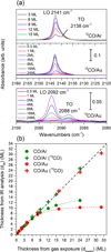 |
Fig. A.1 (a)12CO stretching band for increasing CO exposures (in ML) on Ar (top) and Au (middle); 13CO stretching band on Au (bottom). (b) Number of CO layers (in ML) deduced from the 12CO (circles) and 13CO (crosses) infrared intensities (Eq. A.2), plotted as function of the number of CO layers deduced from the CO gas exposure (Eq. A.1). |
Figure A.1b shows the evolution of IR intensities with gas exposure, calculated using Eq. A.1 with a band strength of A= 1.1 × 1017 cm.molec−1(Jiang et al. 1975; Gerakines et al. 1995; Bouilloud et al. 2015) (uncorrected from the density of the CO ice). Up to 8 ML, the number of CO layers on gold and on argon increases with a linear slope of 1, following the diagonal line. It indicates that the thicknesses calculated from IR intensities match those calculated from gas exposures, i.e., Eq. A.1= Eq. A.2. This confirms the validity of the chosen band strength A in the integration of the LO and TO bands together for estimating the molecular thickness (otherwise the slope would not be 1). This confirms that S = 1 on the argon substrate, otherwise the slope would also not be 1.
Beyond 8 ML, the number of CO layers calculated from IR intensities deviate from linearity (Öberg et al. 2009). This is the result of a combination of reflective and refractive optical effects, which become more important as the layer becomes thicker and the IR absorption increases (Mitlin & Leung 2002; Cholette et al. 2009). This deviation can be empirically modeled with an exponential function (dotted lines in Fig. A.1b), which can be inverted and used as a correction tool. However, this procedure adds an error and more accurate measurements are obtained within the linear range of RAIRS.
The 13CO intensity can also be used for molecular thickness calculations with the same band strength and an isotopic ratio of 12CO/13CO of87 (Bouilloud et al. 2015). The results align well with the diagonal of Fig. A.1b throughout the exposure range, because the optical effects remain negligible for a diluted species which does not absorb much. However, these 13CO bands cannot be used in X-ray irradiation experiments as they overlap with bands from CO byproducts. We then focused our study on CO layers with less than 8 ML of molecular thickness to keep the IR signal of CO linear with thickness.
References
- Arabhavi, A. M., Kamp, I., Henning, T., et al. 2024, Science, 384, 1086 [NASA ADS] [CrossRef] [Google Scholar]
- Basalgète, R., Dupuy, R., Féraud, G., et al. 2021a, A&A, 647, A35 [NASA ADS] [CrossRef] [EDP Sciences] [Google Scholar]
- Basalgète, R., Dupuy, R., Féraud, G., et al. 2021b, A&A, 647, A36 [EDP Sciences] [Google Scholar]
- Basalgète, R., Torres-Diaz, D., Lafosse, A., et al. 2022, J. Chem. Phys., 157, 084308 [CrossRef] [Google Scholar]
- Basalgète, R., Torres-Diaz, D., Lafosse, A., et al. 2023, A&A, 676, A13 [NASA ADS] [CrossRef] [EDP Sciences] [Google Scholar]
- Boogert, A. C., Gerakines, P. A., & Whittet, D. C. 2015, ARA&A, 53, 541 [Google Scholar]
- Bouilloud, M., Fray, N., Bénilan, Y., et al. 2015, MNRAS, 451, 2145 [Google Scholar]
- Bruderer, S., Doty, S. D., & Benz, A. O. 2009, ApJS, 183, 179 [Google Scholar]
- Bulak, M., Paardekooper, D. M., Fedoseev, G., & Linnartz, H. 2020, A&A, 636, A32 [NASA ADS] [CrossRef] [EDP Sciences] [Google Scholar]
- Bulak, M., Paardekooper, D. M., Fedoseev, G., Samarth, P., & Linnartz, H. 2023, A&A, 677, A99 [NASA ADS] [CrossRef] [EDP Sciences] [Google Scholar]
- Carvalho, G. A., & Pilling, S. 2020a, J. Phys. Chem. A, 124, 8574 [Google Scholar]
- Carvalho, G. A., & Pilling, S. 2020b, MNRAS, 498, 689 [Google Scholar]
- Carvalho, G. A., & Pilling, S. 2021, MNRAS, 503, 2973 [Google Scholar]
- Chang, H., Richardson, H. H., Ewing, G. E., et al. 1988, J. Chem. Phys., 89, 7561 [Google Scholar]
- Chantler, C. T. 1995, J. Phys. Chem. Ref. Data, 24, 71 [Google Scholar]
- Chen, Y. J., Ciaravella, A., Muñoz Caro, G. M., et al. 2013, ApJ, 778, 162 [NASA ADS] [CrossRef] [Google Scholar]
- Chen, Y.-J. J., Chuang, K. J., Muñoz Caro, G. M., et al. 2014, ApJ, 781, 15 [Google Scholar]
- Cholette, F., Zubkov, T., Smith, R. S., et al. 2009, J. Phys. Chem. B, 113, 4131 [Google Scholar]
- Chuang, K.-J., Jäger, C., Sie, N.-E., et al. 2023, ApJ, 956, 57 [NASA ADS] [CrossRef] [Google Scholar]
- Ciaravella, A., Muñoz Caro, G., Jiménez Escobar, A., et al. 2010, ApJ, 722, L45 [NASA ADS] [CrossRef] [Google Scholar]
- Ciaravella, A., Jiménez-Escobar, A., Muñoz Caro, G. M., et al. 2012, ApJ, 746, L1 [Google Scholar]
- Ciaravella, A., Chen, Y.-J., Cecchi-Pestellini, C., et al. 2016, ApJ, 819, 38 [Google Scholar]
- Ciaravella, A., Jiménez-Escobar, A., Cecchi-Pestellini, C., et al. 2019, ApJ, 879, 21 [NASA ADS] [CrossRef] [Google Scholar]
- Ciaravella, A., Muñoz Caro, G. M., Jiménez-Escobar, A., et al. 2020, PNAS, 117, 16149 [NASA ADS] [CrossRef] [Google Scholar]
- Ciesla, F. J., & Sandford, S. A. 2012, Science, 336, 452 [NASA ADS] [CrossRef] [Google Scholar]
- Cottin, H., Moore, M. H., & Benilan, Y. 2003, ApJ, 590, 874 [Google Scholar]
- De Souza Bonfim, V., Barbosa De Castilho, R., Baptista, L., & Pilling, S. 2017, Phys. Chem. Chem. Phys., 19, 26906 [Google Scholar]
- Dupuy, R., Bertin, M., Féraud, G., et al. 2018, Nat. Astron., 2, 796 [CrossRef] [Google Scholar]
- Dupuy, R., Féraud, G., Bertin, M., et al. 2020, J. Chem. Phys., 152, 054711 [NASA ADS] [CrossRef] [Google Scholar]
- Dupuy, R., Bertin, M., Féraud, G., et al. 2021, Phys. Chem. Chem. Phys., 23, 15965 [NASA ADS] [CrossRef] [Google Scholar]
- Fayolle, E. C., Bertin, M., Romanzin, C., et al. 2011, ApJ, 739, L36 [Google Scholar]
- Franchy, R., & Menzel, D. 1979, Phys. Rev. Lett., 43, 865 [Google Scholar]
- Freitas, F. M., & Pilling, S. 2020, Quimica Nova, 43, 521 [Google Scholar]
- Frigo, S. P., Feulner, P., Kassühlke, B., Keller, C., & Menzel, D. 1998, Phys. Rev. Lett., 80, 2813 [Google Scholar]
- Gerakines, P. A., & Moore, M. H. 2001, Icarus, 154, 372 [NASA ADS] [CrossRef] [Google Scholar]
- Gerakines, P. A., Schutte, W. A., Greenberg, J. M., & Van Dishoeck, E. F. 1995, A&A, 296, 810 [NASA ADS] [Google Scholar]
- Gerakines, P. A., Schutte, W. A., & Ehrenfreund, P. 1996, A&A, 312, 289 [NASA ADS] [Google Scholar]
- Gerakines, P. A., Hudson, R. L., Moore, M. H., & Bell, J.-L. 2012, Icarus, 220, 647 [Google Scholar]
- He, J. E. T. F., Emtiaz, S. M., Henning, T., & Vidali, G. 2021, ApJ, 915, L23 [NASA ADS] [CrossRef] [Google Scholar]
- Huang, C.-H., Ciaravella, A., Cecchi-Pestellini, C., et al. 2020, ApJ, 889, 57 [NASA ADS] [CrossRef] [Google Scholar]
- Hudgins, D. M., Sandford, S. A., Allamandola, L. J., & Tielens, A. G. 1993, ApJS, 86, 713 [NASA ADS] [CrossRef] [Google Scholar]
- Jamieson, C. S., Mebel, A. M., & Kaiser, R. I. 2006, ApJS, 163, 184 [NASA ADS] [CrossRef] [Google Scholar]
- Jiang, G. J., Person, W. B., & Brown, K. G. 1975, J. Chem. Phys., 62, 1201 [NASA ADS] [CrossRef] [Google Scholar]
- Jiménez-Escobar, A., Chen, Y.-J., Ciaravella, A., et al. 2016, ApJ, 820, 25 [CrossRef] [Google Scholar]
- Jiménez-Escobar, A., Ciaravella, A., Cecchi-Pestellini, C., et al. 2018, ApJ, 868, 73 [Google Scholar]
- Krause, M. 1979, J. Phys. Chem. Ref. Data, 8, 307 [NASA ADS] [CrossRef] [Google Scholar]
- Lacombe, S., Bournel, F., Laffon, C., & Parent, P. 2006, Angew. Chem. Int. Ed., 45, 4159 [Google Scholar]
- Laffon, C., Lacombe, S., Bournel, F., & Parent, P. 2006, J. Chem. Phys., 125, 204714 [Google Scholar]
- Laffon, C., Lasne, J., Bournel, F., et al. 2010, Phys. Chem. Chem. Phys., 12, 10865 [Google Scholar]
- Laidler K. J. 1987, Chemical Kinetics, 3rd edn., ed. Pearson Education (India: Dorling Kindersely (India) Pvt. Ltd.) [Google Scholar]
- Lasne, J., Rosu-finsen, A., Cassidy, A., McCoustra, M. R. S., & Field, D. 2015, Phys. Chem. Chem. Phys., 17, 30177 [Google Scholar]
- Ligterink, N. F., Paardekooper, D. M., Chuang, K. J., et al. 2015, A&A, 584, A56 [NASA ADS] [CrossRef] [EDP Sciences] [Google Scholar]
- Loeffler, M. J., Baratta, G. A., Palumbo, M. E., Strazzulla, G., & Baragiola, R. A. 2005, A&A, 435, 587 [NASA ADS] [CrossRef] [EDP Sciences] [Google Scholar]
- Menzel, D. 2008, Chem. Soc. Rev., 37, 2212 [Google Scholar]
- Mitlin, S., & Leung, K. T. 2002, J. Phys. Chem. B, 106, 6234 [Google Scholar]
- Mizuno, Y., Kofu, M., & Yamamuro, O. 2016, J. Phys. Soc. Jpn., 85, 124602 [Google Scholar]
- Muñoz Caro, G. M., Chen, Y.-J., Aparicio, S., et al. 2016, A&A, 589, A19 [NASA ADS] [CrossRef] [EDP Sciences] [Google Scholar]
- Munõz Caro, G. M., Ciaravella, A., Jiménez-Escobar, A., et al. 2019, ACS Earth Space Chem., 3, 2138 [CrossRef] [Google Scholar]
- Notsu, S., Van Dishoeck, E. F., Walsh, C., Bosman, A. D., & Nomura, H. 2021, A&A, 650, A180 [NASA ADS] [CrossRef] [EDP Sciences] [Google Scholar]
- Öberg, K. I. 2016, Chem. Rev., 116, 9631 [Google Scholar]
- Öberg, K. I., Fuchs, G. W., Awad, Z., et al. 2007, ApJ, 662, L23 [Google Scholar]
- Öberg, K. I., Van Dishoeck, E. F., & Linnartz, H. 2009, A&A, 496, 281 [NASA ADS] [CrossRef] [EDP Sciences] [Google Scholar]
- Paardekooper, D. M., Fedoseev, G., Riedo, A., & Linnartz, H. 2016, A&A, 596, A72 [NASA ADS] [CrossRef] [EDP Sciences] [Google Scholar]
- Palumbo, M. E., Leto, P., Siringo, C., & Trigilio, C. 2008, ApJ, 685, 1033 [NASA ADS] [CrossRef] [Google Scholar]
- Parent, P., & Laffon, C. 2005, J. Phys. Chem. B, 109, 1547 [Google Scholar]
- Parent, P., Laffon, C., Mangeney, C., Bournel, F., & Tronc, M. 2002, J. Chem. Phys., 117, 10842 [Google Scholar]
- Parent, P., Bournel, F., Lasne, J., et al. 2009, J. Chem. Phys., 131, 154308 [NASA ADS] [CrossRef] [Google Scholar]
- Pernet, A., Pilmé, J., Pauzat, F., et al. 2013, A&A, 552, A100 [NASA ADS] [CrossRef] [EDP Sciences] [Google Scholar]
- Pilling, S., & Bergantini, A. 2015, ApJ, 811, 151 [NASA ADS] [CrossRef] [Google Scholar]
- Pilling, S., & da Silva, R. d. C. 2023, Revista Univap, 29, 7 [Google Scholar]
- Pilling, S., & Freitas, F. M. 2023, Revista Univap, 29, 1 [Google Scholar]
- Pilling, S., Rocha, W. R., Freitas, F. M., & Da Silva, P. A. 2019, RSC Adv., 9, 28823 [Google Scholar]
- Pontoppidan, K. M., Fraser, H. J., Dartois, E., et al. 2003, A&A, 408, 981 [NASA ADS] [CrossRef] [EDP Sciences] [Google Scholar]
- Potapov, A., Semenov, D., Jäger, C., & Henning, T. 2023, ApJ, 954, 167 [NASA ADS] [CrossRef] [Google Scholar]
- Rab, C., Güdel, M., Woitke, P., et al. 2018, A&A, 609, A91 [NASA ADS] [CrossRef] [EDP Sciences] [Google Scholar]
- Rachid, M. G., Faquine, K., & Pilling, S. 2017, P&SS, 149, 83 [Google Scholar]
- Sie, N.-E., Cho, Y.-t., Huang, C.-h., et al. 2022, ApJ, 938, 48 [NASA ADS] [CrossRef] [Google Scholar]
- Stadler, C., Laffon, C., & Parent, P. 2024, A&A, 689, A50 [NASA ADS] [CrossRef] [EDP Sciences] [Google Scholar]
- Stäuber, P., Benz, A. O., Jørgensen, J. K., et al. 2007, A&A, 466, 977 [NASA ADS] [CrossRef] [EDP Sciences] [Google Scholar]
- Tielens, A. G. 2005, The Physics and Chemistry of the Interstellar Medium The Physics and Chemistry of the Interstellar Medium (Cambridge: Cambridge University Press), 1 [Google Scholar]
- Tzvetkov, G., & Netzer, F. P. 2011, J. Chem. Phys., 134, 20 [Google Scholar]
- Van Dishoeck, E. F. 2006, PNAS, 103, 12249 [Google Scholar]
- Vasconcelos, F. d. A., Pilling, S., Rocha, W. R. M., Rothard, H., & Boduch, P. 2017, ApJ, 850, 174 [Google Scholar]
- Walsh, C., Millar, T. J., & Nomura, H. 2010, ApJ, 722, 1607 [Google Scholar]
- Walsh, C., Nomura, H., Millar, T. J., & Aikawa, Y. 2012, ApJ, 747, 114 [NASA ADS] [CrossRef] [Google Scholar]
- Walsh, C., Millar, T. J., & Nomura, H. 2013, ApJ, 766, L23 [NASA ADS] [CrossRef] [Google Scholar]
- Walsh, C., Nomura, H., & Van Dishoeck, E. 2015, A&A, 582, A88 [NASA ADS] [CrossRef] [EDP Sciences] [Google Scholar]
- Westley, M. S., Baragiola, R. A., Johnson, R. E., & Barattat, G. A. 1995, Nature, 373, 405 [NASA ADS] [CrossRef] [Google Scholar]
- Zumofen, G. 1978, J. Chem. Phys., 68, 3747 [Google Scholar]
All Tables
UV desorption and dissociation rates at 10 K. The relative error is estimated at 30%.
All Figures
|
Fig. 1 SUMO analysis chamber. (1) Sample position; (2) FTIR spectrometer; (3) FTIR’s MCT detector; (4) X-ray source; (5) UV source; (6) Hemispherical electron analyzer for XPS experiments. |
| In the text | |
|
Fig. 2 Evolution of the CO column densities (from integrated intensity of the 12CO IR band at 2142 and 2138 cm−1) plotted against exposure to UV and X-rays. (a) UV irradiation of CO:Au and Ar:CO:Au ; (b) UV irradiation of CO:Ar and Ar:CO:Ar; (c) X-ray irradiation of CO:Au and Ar:CO:Au ; (d) X-ray irradiation of CO:Ar and Ar:CO:Ar ; at the equilibrium [CO]eq = α[CO]t=0. |
| In the text | |
|
Fig. 3 CO desorption rates: X-rays (top area, red) and UV (bottom area, magenta), updated from the review of Paardekooper et al. (2016), with the addition of our UV and X-ray (1486.6 eV) data, and the X-ray data of Dupuy et al. (2021) taken at 600 eV and scaled at 1486.6 eV (see text). The experimental methods are indicated by the shape of the points: LD TOF-MS is for laser desorption time-of-flight mass spectrometry; NEX-AFS/MS is for NEXAFS spectroscopy coupled with Mass Spectrometry (PSD-NEXAFS). |
| In the text | |
|
Fig. 4 Experimental desorption rates. This work: CO:Ar (blue triangles) at 1486.6 eV (Al Ka) and 1253.6 eV (Mg Ka); Dupuy et al. (2021): Measured at 600 eV (pink star), scaled at 1253.6 eV (pink triangle), scaled at 1486.6 eV (pink circle). Extrapolated rates from the CO X-ray absorption cross section (NIST) (dotted lines) scaled using the desorption rates of CO:Ar at 1486.6 eV (Al Ka). The stripe indicates the margin of error in the NIST data. |
| In the text | |
|
Fig. A.1 (a)12CO stretching band for increasing CO exposures (in ML) on Ar (top) and Au (middle); 13CO stretching band on Au (bottom). (b) Number of CO layers (in ML) deduced from the 12CO (circles) and 13CO (crosses) infrared intensities (Eq. A.2), plotted as function of the number of CO layers deduced from the CO gas exposure (Eq. A.1). |
| In the text | |
Current usage metrics show cumulative count of Article Views (full-text article views including HTML views, PDF and ePub downloads, according to the available data) and Abstracts Views on Vision4Press platform.
Data correspond to usage on the plateform after 2015. The current usage metrics is available 48-96 hours after online publication and is updated daily on week days.
Initial download of the metrics may take a while.