| Issue |
A&A
Volume 700, August 2025
|
|
|---|---|---|
| Article Number | A37 | |
| Number of page(s) | 11 | |
| Section | Astrophysical processes | |
| DOI | https://doi.org/10.1051/0004-6361/202554145 | |
| Published online | 31 July 2025 | |
Supernova remnants in super bubbles acting as cosmic ray accelerators
1
Centro de Investigaciones Energéticas, Medioambientales y Tecnológicas (CIEMAT), E-28040 Madrid, Spain
2
Gran Sasso Science Institute, Via F. Crispi 7, 67100 L’Aquila, Italy
3
INFN-Laboratori Nazionali del Gran Sasso, Via G. Acitelli 22, Assergi, (AQ), Italy
4
Centre for Space Research, North-West University, 2520 Potchefstroom, South Africa
5
Astronomical Observatory of Ivan Franko National University of Lviv, Kyryla i Methodia 8, 79005 Lviv, Ukraine
6
Institute of Physics and Astronomy, University of Potsdam, 14476 Potsdam-Golm, Germany
7
School of Physical Sciences and Centre for Astrophysics & Relativity, Dublin City University, Glasnevin D09 W6Y4, Ireland
⋆ Corresponding author: This email address is being protected from spambots. You need JavaScript enabled to view it.
Received:
14
February
2025
Accepted:
31
May
2025
Abstract
Supernova remnants (SNRs) are often considered the main sites of acceleration of cosmic rays in our Galaxy, possibly up to the ‘knee’. However, their ability to accelerate particles to reach PeV energies is questionable and lacks observational evidence. Theoretical predictions suggest that only a small sub-class of very young SNRs evolving in dense environments could potentially satisfy the necessary conditions to accelerate particles to PeV energies. Most theoretical investigations of this type have been carried out either in the standard interstellar medium or in the wind of the progenitor. Since most core-collapse supernovae (CC SNe) occur in star clusters, it is important to extend such investigations to SNRs taking place within a star cluster. In this work, we focus on an SNR shock propagating in the collective wind of a compact star cluster. We studied the acceleration process as a function of time, with a special emphasis on the maximum energy of accelerated particles. Using both analytic and numerical approaches, we investigated the spectrum of accelerated particles and maximum achievable energy in the case of pre-existing turbulence in the collective wind and self-generated magnetic perturbations. We find that similarly to the case of isolated SNRs, the acceleration to PeV energies is plausible only in extreme conditions that are achievable only for a small sub-set of SNRs.
Key words: acceleration of particles / shock waves / cosmic rays / ISM: supernova remnants / galaxies: star clusters: general
© The Authors 2025
 Open Access article, published by EDP Sciences, under the terms of the Creative Commons Attribution License (https://creativecommons.org/licenses/by/4.0), which permits unrestricted use, distribution, and reproduction in any medium, provided the original work is properly cited.
This article is published in open access under the Subscribe to Open model. This email address is being protected from spambots. You need JavaScript enabled to view it. to support open access publication.
1. Introduction
Supernova remnants (SNRs) have long been considered as the main candidates to be sources of the bulk of Galactic cosmic rays (CRs), mainly on the basis of energetic arguments. Gamma-ray observations provide indirect proof that SNRs can accelerate particles to energies as high as ∼10 − 100 TeV (Ackermann et al. 2013; Giuliani & AGILE Team 2011; Jogler & Funk 2016; Ambrogi et al. 2019; de Oña Wilhelmi et al. 2020), implying that SNRs certainly are important contributors to the CR sea at low energies. However, the shape of the CR spectrum, in particular the distinct ‘knee’ spectral feature at ∼3 PeV, strongly suggests that protons should be accelerated to at least PeV energies within our Galaxy. Moreover, if the transition from Galactic to extragalactic CRs occurs in fact at ∼1017 eV (at the less pronounced ‘second knee’ in the CR spectrum), then Galactic sources should be able to accelerate protons beyond 10 PeV (see Vieu & Reville 2023, and references therein). In addition to the lack of observational evidence for SNRs as PeVatrons, there is also a growing theoretical consensus that only exceptionally energetic SNRs or very young SNRs (tens of years after explosion) in specific environments might accelerate protons to the knee region (Marcowith et al. 2018; Cristofari et al. 2020a,b; Inoue et al. 2021; Brose et al. 2022, 2025; Diesing 2023).
Several other source types have been proposed to take over at PeV energies. Among these, the most promising in the light of recent observations seem to be young compact star clusters (Aharonian et al. 2019, 2022; Abeysekara et al. 2021; LHAASO Collaboration 2024a) and microquasars (H.E.S.S. Collaboration 2024; Alfaro et al. 2024; LHAASO Collaboration 2024b). The former is interesting in the context of the SNR paradigm because one of the scenarios considered for particle acceleration in these objects is the SNR evolving in the bubble generated by the collective wind from the massive stars in the cluster. Vieu et al. (2022a) proposed that the SNR shock expanding into the collective wind with pre-existing magnetic turbulence advected from the cluster could accelerate particles to ∼10 PeV without the need for additional self-generated magnetic field amplification. This scenario is also attractive because it seems to be able to accommodate the composition of CRs which is different from the solar one. In particular, the ratio of 22Ne to 20Ne, which is about five times higher than the solar value (see e.g. Binns et al. 2008) could be explained by the enrichment of the super bubble environment with Wolf-Rayet winds (Gupta et al. 2020). The majority of massive stars reside in clusters, strongly suggesting that most core-collapse supernovae (CC SNe) occur in stellar clusters (Parizot et al. 2004; Portegies Zwart et al. 2010). Unambiguous observational evidence is lacking mainly due to the fact that SNe are not particularly frequent events and the capabilities of instruments to detect star cluster counterparts are limited to nearby galaxies (Portegies Zwart et al. 2010). One of the most prominent associations reported is the type IIp supernova SN2004dj, which is believed to occur in the star cluster Sandage-96 in the spiral galaxy NGC 2403 (Wang et al. 2005). Nevertheless, if this is the case, it is expected that a large fraction of SNRs are evolving in super bubbles with an environment potentially favourable for effective particle acceleration. However, no detailed simulations have been available so far that would quantitatively confirm acceleration of particles to PeV energies in such an environment.
There are several potential sites of particle acceleration and subsequent non-thermal emission in super bubbles (see e.g. Parizot et al. 2004) and existing observations do not offer an unambiguous preference for any of them. Particles can be accelerated inside cores of stellar clusters through shock re-acceleration, shock collisions, and stochastic re-acceleration; however, recent simulations have shown that these processes are ineffective in boosting the maximum energy of accelerated particles (Vieu et al. 2024a). There is also no observational evidence of high-energy emission from the cores. Some clusters, such as Westerlund 1, exhibit a shell-like morphology of the associated gamma-ray emission (Aharonian et al. 2022). For those exhibiting a centrally filled morphology (e.g. Cygnus OB2), the angular resolution of the available instruments does not allow for a firm identification of the emission with the core (Aharonian et al. 2019).
Another potential site of effective particle acceleration which also has some observational support is the termination shock of the collective wind of the stellar cluster. For instance, H.E.S.S. observations of Westerlund 1 show the shell-like morphology of the gamma-ray emission with the radial distance to the peak of the gamma-ray emission of ∼34 pc that shows a good agreement with the estimate of the radius of the termination shock (Aharonian et al. 2022). In this framework, Härer et al. (2023) advocated for a leptonic scenario where most gamma ray emission is due to inverse Compton scattering of high-energy electrons accelerated at the termination shock, whereas the contribution of hadronic interactions was estimated to be negligible under standard assumptions. It remains to be seen whether this scenario is compatible with the absence of radio emission and with the morphology of the gamma-ray emission. From the theoretical point of view, Morlino et al. (2021) showed that acceleration at the termination shock can be efficient, but PeV energies can be reached only for rather bright star clusters with very fast outflows and only for Bohm diffusion, whereas for Kolmogorov and Kraichnan diffusion, the effective maximum energy falls short of the 1 PeV mark.
It is also possible that particles could be accelerated in the super bubble downstream of the termination shock through second-order Fermi acceleration. It has been argued that a high level of turbulence and high Alfvén velocity could significantly speed up this acceleration mechanism; however, similarly to the acceleration at the termination shock even for optimistic considerations, PeV energies are achievable only for Bohm diffusion (Vink 2024), which is a rather unrealistic description of the turbulence in the super bubble.
In the following, we analyse in depth the remaining scenario linked to the evolution of the putative SNR exploded at the edge of the star cluster core and expanding into the turbulent magnetised environment of the star cluster super bubble. The main objective of the study is to critically assess the ability of an SNR evolving in a super bubble to accelerate particles to energies beyond the knee. We consider the most favourable scenario, whereas the putative SNR is the remnant of the first SN explosion in the star cluster and the star cluster is compact enough to produce a collective wind. It is also expected that the most effective acceleration would happen at a relatively young age of an SNR before the forward shock reaches the termination shock and slows down considerably. It should be noted that although a SN explosion in a young massive stellar cluster is unavoidable and its occurrence at the edge of a cluster is quite probable, there is very limited observational evidence of SNRs identified within super bubbles, especially for the cases where efficient particle acceleration is confirmed through X-ray and/or gamma-ray observations. This is partly due to the difficulties of simultaneous detection of both objects and reliable association with each other and partly due to the selection bias linked to the fact that the whole lifetime of an SNR is only a small fraction of the lifespan of the stellar cluster. Nevertheless, in some cases, convincing arguments have been put forward to support the notion that we could indeed be witnessing the evolution of an SNR inside the super bubble generated by the stellar cluster. For example, X-ray emission associated with the super bubble 30 Dor C in the Large Magellanic Cloud requires high shock velocities, which strongly suggests that this emission is generated by an SNR within the super bubble (Bamba et al. 2004; Yamaguchi et al. 2009; H.E.S.S. Collaboration 2015). However, the picture would depict late stages of the evolution of the SNR, when it starts to interact with the outer shell of the super bubble.
The paper is structured as follows. In Section 2.1, we describe the environment in which the remnant evolves, in Section 3 we provide analytic calculations of the maximum energy based on different assumptions for the magnetic turbulence responsible for the confinement of particles at the shock, in Section 4 we describe the numerical set-up and present the results on numerical simulations using the RATPaC software, and in Section 5 we summarise and discuss our findings.
2. The ambient medium
2.1. Collective wind
In the following, we consider a SN exploding at the edge of the core of the young compact stellar cluster, where we assume that no previous explosions occurred (see Fig. 1 for a schematic cartoon depicting the scenario considered). The SNR shock expands into the medium shaped by the collective wind of the stars in the stellar cluster. Typically, stellar clusters contain under 100 SN progenitors (Lingenfelter 2018), while the most massive stellar clusters may contain up to several thousand massive stars (see e.g. Krumholz et al. 2019). The most massive stellar cluster in the Milky Way, Westerlund 1, hosts at least 166 stars with initial masses between ∼25 M⊙ ∼50 M⊙ – out of which 24 are classified as Wolf-Rayet stars (Clark et al. 2020). The first SN explosion takes place at an age of around 3 million years. The average mechanical power of the collective wind of the cluster consisting of 100 stars throughout its evolution is of the order of ∼1038 erg/s (Vieu et al. 2022b). In the following, we consider the total mass-loss rate of Ṁ = 2 × 10⁻⁴ M⊙/yr and wind velocity of vw = 3 × 108 cm/s, which is equivalent to 100 typical Wolf-Rayet or very luminous main-sequence stars and corresponds to the total wind power of  erg/s. The choice of parameters is identical to the Model 4 considered for Cygnus OB2 in Blasi & Morlino (2023). The location of the termination shock can be approximated (Morlino et al. 2021; Blasi & Morlino 2023) via
![Mathematical equation: $$ \begin{aligned} R_\mathrm{TS} \simeq &21 \left[\frac{\dot{M}}{2\times 10^{-4} \,M_\odot /\mathrm{yr} }\right]^{3/10}\left[\frac{n_\mathrm{ISM} }{10\,\mathrm{cm} ^{-3}}\right]^{-3/10}\nonumber \\&\times \left[\frac{v_\mathrm{w} }{3\times 10^8\,\mathrm{cm/s} }\right]^{1/10} \left[\frac{t}{3\times 10^6\,\mathrm{yr}}\right]^{2/5}\,\mathrm{pc} , \end{aligned} $$](/articles/aa/full_html/2025/08/aa54145-25/aa54145-25-eq2.gif) (1)
(1)
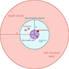 |
Fig. 1. Schematic cartoon illustrating the considered scenario. Note: the ratios of the relevant length scales, i.e. the radius of the core, Rc, the radius of the termination shock, RTS, and the radius of the outer shock, Rb, do not reflect the real proportions. |
which is in agreement within ≲10% with a more accurate Weaver et al. (1977) calculation. The position of the outer shock of the bubble can be approximated by
![Mathematical equation: $$ \begin{aligned} R_\mathrm{b} \simeq &120 \left[\frac{\dot{M}}{2\times 10^{-4}\,M_\odot /\mathrm{yr} }\right]^{1/5}\left[\frac{n_\mathrm{ISM} }{10\,\mathrm{cm} ^{-3}}\right]^{-1/5}\nonumber \\&\times \left[\frac{v_\mathrm{w} }{3\times 10^8\,\mathrm{cm/s} }\right]^{2/5} \left[\frac{t}{3\times 10^6\,\mathrm{yr}}\right]^{3/5}\,\mathrm{pc} . \end{aligned} $$](/articles/aa/full_html/2025/08/aa54145-25/aa54145-25-eq3.gif) (2)
(2)
The gas density in the wind region can be written as
 (3)
(3)
up to the termination shock. Downstream of the shock, the density is assumed to be constant, while the velocity of the shocked wind drops as ∝r−2. These trends are to be considered as valid descriptions of the wind for compact stellar clusters, while non-compact clusters might have a complex outflow that, however, cannot be described in terms of a collective wind. In fact, this might be the case for Cygnus OB2, where 3D hydrodynamic simulations based on the observed stellar population suggest that a collective wind is not actually formed (Vieu et al. 2024b).
2.2. Magnetic field and pre-existing turbulence
A fraction of the kinetic energy of the winds of individual stars is expected to be converted into magnetic turbulence through wind-wind collisions. This turbulence is advected with the collective wind and compressed at the termination shock. It is, however, unclear how much of the total kinetic energy of winds is dissipated and what the level of magnetic turbulence is. Numerical 3D MHD simulations show that the magnetic field in the stellar cluster core is non-uniform, reaching values of 1 μG with the mean value of the magnetic field reaching 200 μG and the median value reaching 35 μG (Härer et al. 2025).
It should be understood that the collective wind parameters set above already account for part of the total kinetic energy being converted into turbulence. Assuming passive transport of the turbulent magnetic field with the flow and ignoring any potential damping, the turbulent field can be written as
 (4)
(4)
where Bc is the generated turbulent field at the edge of the cluster core at the radius of Rc and  is the compression factor at the termination shock. The 3D MHD simulations presented in Härer et al. (2025) confirm that the magnetic field is indeed scaled as approximately 1/r in the collective wind. The magnetic field is assumed to remain constant in the bubble downstream of the termination shock, which should be considered as an optimistic scenario because the turbulent field could be subjected to significant damping. The total energy in the turbulent magnetic field can be estimated as
 (5)
(5)
This can be compared to the total energy in the wind calculated as
![Mathematical equation: $$ \begin{aligned} E_\mathrm{wind} = 5.7\times 10^{52} \left[\frac{L_\mathrm{w} }{6\times 10^{38}\,\mathrm{erg/s} }\right] \left[\frac{t}{3\times 10^6\,\mathrm{yr}}\right]\,\mathrm{erg} . \end{aligned} $$](/articles/aa/full_html/2025/08/aa54145-25/aa54145-25-eq8.gif) (6)
(6)
Setting Eturb = ηE(Ewind + Eturb) and assuming Rc = 1 pc, we can estimate the strength of the turbulent magnetic field at the edge of the core for adopted parameters of the wind as
 (7)
(7)
for ηE = 0.1.
Alternatively, we could constrain Bc by assuming that the magnetic energy density at the edge of the core constitutes a fraction of the wind energy as
 (8)
(8)
For assumed parameters of the collective wind the turbulent magnetic field at the edge of the core for ηw = 0.1 is
 (9)
(9)
Since this magnetic field is assumed to be created through the dissipation of the winds of the many stars in the core, it is expected to be turbulent, on some coherence scale, and it eventually cascades to smaller scales. These estimates are in agreement with the mean values obtained in 3D MHD simulations, but they are higher than the bulk magnetic field strength represented by the median values (Härer et al. 2025). For the radius of the termination shock of ∼20 pc (see Section 2.1), the estimated value of Bc ∼ 200 μG corresponds to ∼10 μG at the termination shock and to ∼30 μG in the super bubble downstream of the termination shock. The available measurements suggest lower values of the magnetic field: B ≈ 3 − 10 μG in Orion-Eridanus (Joubaud et al. 2019) and B ≈ 10 − 20 μG in 30 Dor C (Kavanagh et al. 2019). In this context, by adopting B = 10 μG in the immediate upstream of the termination shock, we can explore the high end of the parameter space, which allows us to reach the highest maximum energies possible.
3. Estimates of the maximum energy
3.1. Pre-existing turbulence
We assume that the turbulence is generated at the coherence scale of L = 1 pc, which corresponds to the assumed radius of the core. Furthermore, we assume that the turbulence evolves following either the Kolmogorov or Kraichnan cascade (hereafter referred to as KOLM and KRAI). The diffusion coefficient for these two cases can be expressed as
 (10)
(10)
 (11)
(11)
where rL = pc/(eB) is the Larmor radius of the particle with a momentum, p, and v is the particle velocity.
The maximum energy that can be achieved in the acceleration process can be estimated, limiting the acceleration time with the age of the remnant. The energy gain rate of the particle can be written as (see e.g. Lagage & Cesarsky 1983):
 (12)
(12)
where  is the energy gain per one acceleration cycle and
  is the cycle time interval. The upstream and downstream regions are denoted by sub-scripts 1 and 2, respectively, with u being the plasma velocity and D the diffusion coefficient. For u1 = vs and assuming a strong shock with the compression ratio of u1/u2 = 4 this can be further rewritten as
 (13)
(13)
For fully isotropic turbulence the magnetic field downstream is compressed by a factor of  , because the radial component of the field is not compressed. Taking into account the dependence of the diffusion coefficient on the magnetic field (see Eqs. (10) and (11)), the relation of the downstream to upstream diffusion coefficient for the two cases of the turbulence spectrum can be estimated as
 (14)
(14)
 (15)
(15)
Then assuming that the evolution of the SNR shock is given by
 (16)
(16)
and
 (17)
(17)
the maximum energy for the two cases can be estimated by integration of Eq. (13) as
![Mathematical equation: $$ \begin{aligned} E_\mathrm{max} ^\mathrm{KOLM} = 23 \left(\frac{j}{5j-3}\right)^3&\left[\frac{t}{t_\mathrm{TS} }\right]^{5j-3} \left[\frac{L}{1\,\mathrm{pc} }\right]^{-2} \left[\frac{R_\mathrm{TS} }{20\,\mathrm{pc} }\right]^3\nonumber \\&\left[\frac{v_\mathrm{TS} }{10^9\,\mathrm{cm/s} }\right]^{3} \left[\frac{B_\mathrm{TS} }{10\,\upmu \mathrm{G} }\right]\,\mathrm{TeV} , \end{aligned} $$](/articles/aa/full_html/2025/08/aa54145-25/aa54145-25-eq23.gif) (18)
(18)
![Mathematical equation: $$ \begin{aligned} E_\mathrm{max} ^\mathrm{KRAI} = 227 \left(\frac{j}{3j-2}\right)^2&\left[\frac{t}{t_\mathrm{TS} }\right]^{3j-2} \left[\frac{L}{1\,\mathrm{pc} }\right]^{-1} \left[\frac{R_\mathrm{TS} }{20\,\mathrm{pc} }\right]^2\nonumber \\&\left[\frac{v_\mathrm{TS} }{10^9\,\mathrm{cm/s} }\right]^{2} \left[\frac{B_\mathrm{TS} }{10\,\upmu \mathrm{G} }\right]\,\mathrm{TeV} , \end{aligned} $$](/articles/aa/full_html/2025/08/aa54145-25/aa54145-25-eq24.gif) (19)
(19)
normalising the parameters to the values at the time, tTS, when the shock reaches the termination shock with RTS and vTS being the shock radius and velocity at that time, while BTS is the magnetic field upstream the termination shock. For a CC SNR evolving in the free wind at the free-expansion stage, j = 6/7 is typically assumed1. After adopting this value, Eqs. (18) and (19) can be rewritten as
![Mathematical equation: $$ \begin{aligned} E_\mathrm{max} ^\mathrm{KOLM}&= 7\,\mathrm{TeV} ,\nonumber \\&\;\;\left[\frac{t}{t_\mathrm{TS} }\right]^{9/7} \left[\frac{L}{1\,\mathrm{pc} }\right]^{-2} \left[\frac{R_\mathrm{TS} }{20\,\mathrm{pc} }\right]^3 \left[\frac{v_\mathrm{TS} }{10^9\,\mathrm{cm/s} }\right]^{3} \left[\frac{B_\mathrm{TS} }{10\,\upmu \mathrm{G} }\right], \end{aligned} $$](/articles/aa/full_html/2025/08/aa54145-25/aa54145-25-eq25.gif) (20)
(20)
![Mathematical equation: $$ \begin{aligned} E_\mathrm{max} ^\mathrm{KRAI}&= 510\,\mathrm{TeV} ,\nonumber \\&\;\;\left[\frac{t}{t_\mathrm{TS} }\right]^{4/7} \left[\frac{L}{1\,\mathrm{pc} }\right]^{-1} \left[\frac{R_\mathrm{TS} }{20\,\mathrm{pc} }\right]^2 \left[\frac{v_\mathrm{TS} }{10^9\,\mathrm{cm/s} }\right]^{2} \left[\frac{B_\mathrm{TS} }{10\,\upmu \mathrm{G} }\right]. \end{aligned} $$](/articles/aa/full_html/2025/08/aa54145-25/aa54145-25-eq26.gif) (21)
(21)
In both cases, the maximum energy increases with time until the SN shock reaches the termination shock. reaching its peak at the termination shock. At this point, although it could be the case that the SN shock is not yet in the Sedov phase at this time, the shock velocity drops considerably due to the higher density downstream of the termination shock, so that eventually the Sedov phase is entered shortly after. Furthermore, the high pressure and temperature of the shocked wind would result in a considerable reduction of the shock Mach number and a correspondingly smaller compression ratio at the SN shock. This combination of events causes a softer spectrum of freshly accelerated particles, so that even if the maximum energy may slightly increase, it does not show in the overall spectrum of accelerated particles.
One last point to keep in mind is that in pre-existing turbulence, the maximum energy is also limited by the largest scale of the turbulence, namely, the coherence scale, L. Particles with a gyroradius larger than L perform a small deflection transport, so that their maximum energy cannot increase further. This additional criterion leads to the following constraint on the maximum energy (Blasi & Morlino 2023):
![Mathematical equation: $$ \begin{aligned} E_\mathrm{max} = eBL = 9.2 \left[\frac{B_\mathrm{TS} }{10\,\upmu \mathrm{G} }\right] \left[\frac{L}{1\,\mathrm{pc} }\right]\,\mathrm{PeV} . \end{aligned} $$](/articles/aa/full_html/2025/08/aa54145-25/aa54145-25-eq27.gif) (22)
(22)
This constraint implies that even when decreasing the coherence scale in Eqs. (20) and (21), this does not necessarily lead to a higher maximum energy.
3.2. Self-generated turbulence
The previous section leads to the conclusion that pre-existing turbulence alone is not sufficient to accelerate particles to PeV energies at the SNR shock. Therefore, here we consider the possibility that the accelerated particles may drive additional self-generated perturbations through excitation of resonant and non-resonant streaming instabilities, which might help reach higher maximum energies.
In the bubble excavated by the wind, it is hard to imagine the existence of any regular magnetic fields, although we could consider a local direction where the field is roughly well behaved on a scale of the order of ∼L, which represents the coherence scale of the turbulent field introduced above. On such scales, local CR gradients can excite the streaming instability. Given the many assumptions adopted here, it is fair to take the results below as some sort of estimate of the effects expected due to the excitation of instabilities.
The diffusion coefficient written in quasi-linear theory is expressed as (Bell 1978):
 (23)
(23)
where ℱ is the energy density of Alfven waves per unit logarithmic bandwidth scaled to the energy density of the background magnetic field. We also introduced a parameter expressed as ηB ≡ 1/ℱ ≥ 1 to characterize the deviations from pure Bohm diffusion. The resonant streaming instability operates on a time scale that is the crossing time of the precursor of particles with a momentum, p, at the shock speed, which results in the following estimate for the ℱ, for the canonical p−4 spectrum of accelerated particles (Amato & Blasi 2006):
 (24)
(24)
where Λ = ln(pmax/mpc)∼10. The corresponding magnetic field strength induced by the instability (Amato & Blasi 2006) is expressed as
 (25)
(25)
where  is the local Alfvén velocity and η is the particle injection efficiency defined as the fraction of the ram pressure, ρvs2, converted to CRs: η = PCR/(ρvs2).
Combining the equations above and using the expression in Eq. (3) for the density in the collective wind, we can write ηB as
 (26)
(26)
and taking into account evolution of the shock and spatial dependence of the magnetic field in the collective wind
 (27)
(27)
For the parameters considered here ηB can be estimated as
![Mathematical equation: $$ \begin{aligned} \eta _\mathrm{B}&= 4.8 \left[\frac{\eta }{0.1}\right]^{-1} \left[\frac{\Lambda }{10}\right] \left[\frac{\dot{M}}{2\times 10^{-4}\,M_\odot /\mathrm{yr} }\right]^{-1/2}\nonumber \\&\left[\frac{v_\mathrm{w} }{3\times 10^8\,\mathrm{cm/s} }\right]^{1/2} \left[\frac{v_\mathrm{TS} }{10^9\,\mathrm{cm/s} }\right]^{-1} \left[\frac{R_\mathrm{TS} }{20\,\mathrm{pc} }\right] \left[\frac{B_\mathrm{TS} }{10\,\upmu \mathrm{G} }\right] \left[\frac{t}{t_\mathrm{TS} }\right]^{1-j}. \end{aligned} $$](/articles/aa/full_html/2025/08/aa54145-25/aa54145-25-eq34.gif) (28)
(28)
A note of caution is in order: although typically ηB ≳ 1, we can see that δB ∼ B, which stretches the validity of this treatment to its limits. The resonant streaming instability is expected to be saturated when δB/B ∼ 1, as a consequence of the requirement that a resonance between waves and particle gyration is fulfilled. When this happens, the most reasonable option is to assume that the diffusion coefficient becomes Bohm-like with δB = B. With these limitations, we can follow the same line of reason outlined above and express the following:
 (29)
(29)
alternatively, if ηB is constant in time,
 (30)
(30)
It should be noted that in contrast to the case of KOLM and KRAI turbulence, the energy gain seen here decreases over time faster than ∝1/t for j < 1, implying that the maximum energy would depend on the time when the particles are injected into the acceleration process. This is a very peculiar situation because of the fast decrease of the magnetic field with the distance from the origin and the rapid (linear) energy increase of the diffusion coefficient. Essentially, this means that the instantaneous maximum energy would decrease with time and particles injected at later stages will not be accelerated to energies as high as those injected at the very beginning. Hence, although the particles injected at the beginning will continue to gain energy, the effective maximum energy will decrease with time.
Integrating Eq. (29) from the injection time, tinj, to t results in a dependence expressed as
 (31)
(31)
where for j < 1 and tinj ≪ t the maximum achievable energy of an injected particle would depend only on the time of injection. For particles injected at a time, tinj ≪ tTS, the maximum achievable energy can be estimated as
![Mathematical equation: $$ \begin{aligned} E_\mathrm{max} \simeq 153 \,\frac{j}{2-2j}&\left[\frac{t_\mathrm{inj} }{t_\mathrm{TS} }\right]^{2j-2}\left[\frac{\eta }{0.1}\right]\left[\frac{\Lambda }{10}\right]^{-1}\left[\frac{\dot{M}}{2\times 10^{-4}\,M_\odot /\mathrm{yr} }\right]^{1/2}\nonumber \\&\left[\frac{v_\mathrm{w} }{3\times 10^8\,\mathrm{cm/s} }\right]^{-1/2} \left[\frac{v_\mathrm{TS} }{10^9\,\mathrm{cm/s} }\right]^{2}\,\mathrm{TeV} \end{aligned} $$](/articles/aa/full_html/2025/08/aa54145-25/aa54145-25-eq38.gif) (32)
(32)
or, for j = 6/7,
![Mathematical equation: $$ \begin{aligned} E_\mathrm{max} \simeq 456\,&\left[\frac{t_\mathrm{inj} }{t_\mathrm{TS} }\right]^{-2/7}\left[\frac{\eta }{0.1}\right]\left[\frac{\Lambda }{10}\right]^{-1}\left[\frac{\dot{M}}{2\times 10^{-4}\,M_\odot /\mathrm{yr} }\right]^{1/2}\nonumber \\&\left[\frac{v_\mathrm{w} }{3\times 10^8\,\mathrm{cm/s} }\right]^{-1/2} \left[\frac{v_\mathrm{TS} }{10^9\,\mathrm{cm/s} }\right]^{2} \,\mathrm{TeV} . \end{aligned} $$](/articles/aa/full_html/2025/08/aa54145-25/aa54145-25-eq39.gif) (33)
(33)
Unfortunately, these expressions are not of much help in that they suggest that the particles that are accelerated to the highest energies are injected at times where the amount of mass processed by the shock is small. Moreover, if the resonant instability regime operates on top of the pre-generated turbulence, the energy gain at later stages could be actually controlled by the KRAI or KOLM diffusion, allowing the maximum energy to keep growing. It is worth stressing that these estimates of the maximum energy apply to individual particles, while the maximum energy that appears in the spectrum of accelerated particles also reflects the amount of mass processed during the acceleration process. Only a numerical calculation such as the one discussed below can purposefully address this issue. It should be noted that these estimates differ considerably from the similar analysis adopted by Vieu & Reville (2023), suggesting that typical SNRs evolving in the wind bubble of the stellar cluster could accelerate particles to ∼4 PeV under the assumption of Bohm diffusion. In addition to a different choice for ηB which they set to unity, a major difference in their treatment is the assumption of constant shock velocity, which essentially implies that the maximum energy would not depend on the injection time.
The situation is going to be somewhat different once the SNR shock reaches the termination shock and starts propagating in the hot bubble of the shocked wind. Assuming that the density and the magnetic field remain constant in the downstream of the termination shock, the energy gain will evolve with time as
 (34)
(34)
If the SNR still remains in the free-expansion stage of its evolution, (i.e. j = 2/3 for expansion in a medium with constant density), the energy gain will decrease with time as ∝1/t and, hence, Emax would stay constant. On the other hand, as soon as the SNR transitions to the Sedov-Taylor stage, the shock starts to slow down faster, with j = 2/5, and the energy gain starts to decrease as ∝t−9/5 leading to saturation of the value of the effective maximum energy. Other effects are also expected to play an important role. In particular, the interaction of the SNR shock with the termination shock results in the formation of a reflected shock which after bouncing off the contact discontinuity inside the remnant would catch up with the forward shock, accelerating it and leading to a slight increase in the maximum energy of the accelerated particles (Sushch et al. 2022). Another important effect is the weakening of the shock due to the high temperature of the medium which results in a softer spectrum of the accelerated particles (Das et al. 2022). At this point, a negligibly small fraction of the accelerated particles can reach very high energies. Both of these effects are further discussed below in the context of numerical simulations.
So far, we have discussed the effects of the excitation of the resonant streaming instability, but in the case of fast SNR shocks, a non-resonant instability is also expected to grow (Bell 2004), provided that the following condition is met:
 (35)
(35)
For fast SNR shocks, the growth of the non-resonant instability is typically faster than the resonant branch. The condition above can be translated into the upper limit on the background magnetic field in the collective wind for the instability to grow:
![Mathematical equation: $$ \begin{aligned} B&< 1.92 \left[\frac{\eta }{0.1}\right]^{1/2}\left[\frac{\Lambda }{10}\right]^{-1/2} \left[\frac{\dot{M}}{2\times 10^{-4}\,M_\odot /\mathrm{yr} }\right]^{1/2}\nonumber \\&\left[\frac{v_\mathrm{w} }{3\times 10^8\,\mathrm{cm/s} }\right]^{-1/2} \left[\frac{v_\mathrm{TS} }{10^9\,\mathrm{cm/s} }\right]^{3/2} \left[\frac{R_\mathrm{TS} }{20\,\mathrm{pc} }\right]^{-1} \left[\frac{t}{t_\mathrm{TS} }\right]^{(j-3)/2}\,\upmu \mathrm{G} . \end{aligned} $$](/articles/aa/full_html/2025/08/aa54145-25/aa54145-25-eq42.gif) (36)
(36)
A comparison with the magnetic fields expected from a ∼10% conversion efficiency from the kinetic energy of the wind (Blasi & Morlino 2023) immediately suggests that in order for this non-resonant instability to grow this efficiency must be appreciably smaller than ∼10%. If this is the case, then the magnetic field produced at saturation of the non-resonant instability is the same as given in the RHS of Eq. (36), due to the way this instability works. Moreover, if the spectrum of accelerated particles is canonical p−4, then the diffusion coefficient is Bohm-like in the amplified magnetic field (Cristofari et al. 2020a, 2021) and it could easily be smaller (faster acceleration) than in the case of resonant instability considered above. A somewhat more stringent condition on the amplified magnetic field is also obtained based on the condition that the non-resonant instability grows fast enough in a given time, t (Schure & Bell 2014). Since we are not considering the case of non-resonant instability below, we do not provide additional details, which can be found in the articles cited above.
Finally, magnetic field amplification can occur because of a sort of kinematic dynamo effect (Drury & Downes 2012; Beresnyak et al. 2009): vorticity can be induced in a plasma where density fluctuations are present, in the presence of a CR pressure gradient. The amplified magnetic field can then be estimated as (Drury & Downes 2012):
 (37)
(37)
and assuming that the instability drives toward density fluctuations of order unity, δρ/ρ ∼ 1, the equation above becomes  , which is typically ∼3 − 30 times larger than the energy density potentially provided by the non-resonant instability. In the following, we consider Bohm diffusion in a magnetic field amplified in this way as the most optimistic case of particle acceleration.
4. Numerical simulations
4.1. Numerical set-up
Numerical simulations of particle acceleration at a SNR shock evolving in the super bubble created by the compact stellar cluster were performed using the Radiation Acceleration Transport Parallel Code (RATPaC). The code is designed for the temporally and spatially dependent treatment of transport of cosmic rays in SNRs. Initially, the code relied on the assumption of Bohm-like diffusion and analytic or pre-calculated numeric treatment of the hydrodynamic evolution (Telezhinsky et al. 2012, 2013), while more recently the modules for solving the transport equation for magnetic turbulence (Brose et al. 2016) and hydrodynamic simulations on-the-fly (Sushch et al. 2018; Brose et al. 2019) were introduced. We summarise the numerical set-up used in this work below.
4.1.1. Hydrodynamics
To describe the evolution of the SNR in the ambient medium, we solved the standard gas-dynamical equations ignoring the feedback of cosmic rays and the magnetic field on the evolution.
 (38)
(38)
 (39)
(39)
where ρ is the density of the thermal gas, v the plasma velocity, m = vρ the momentum density, P is the thermal pressure of the gas, and E the total energy density of the ideal gas with γ = 5/3. This system of equations is solved under the assumption of spherical symmetry in 1D using the PLUTO code (Mignone et al. 2007).
The ejecta profile is initialized by a constant density, ρc, up to the radius, rc, followed by a power-law distribution up to the ejecta-radius Rej,
 (40)
(40)
beyond which the density profile is that of the star cluster super bubble described below. The exponent for the ejecta profile is set to n = 9. The velocity of the ejecta is defined as
 (41)
(41)
where TSN = 1 yr is the initial time set for hydrodynamic simulations. Defining the radius of the ejecta as multiple of rc, Rej = xrc with x = 3, the initial conditions for simulations can be written as
![Mathematical equation: $$ \begin{aligned} r_c&= \left[\frac{10}{3}\frac{E_{\mathrm{ej} }}{M_{\mathrm{ej} }} \left(\frac{n-5}{n-3}\right) \left(\frac{1- \frac{3}{n} x^{3-n}}{1-\frac{5}{n} x^{5-n}}\right)\right]^{1/2} T_{\mathrm{SN} }, \end{aligned} $$](/articles/aa/full_html/2025/08/aa54145-25/aa54145-25-eq49.gif) (42)
(42)
 (43)
(43)
 (44)
(44)
In the following, the ejecta mass is assumed to be Mej = 3 M⊙ and for the explosion energy we consider two cases: ‘classic’ with Eej = 1051 erg and ‘energetic’ with Eej = 1052 erg.
We assume that the SNR explodes right on the edge of the star-cluster core with Rc = 1 pc. We re-define the spatial coordinate as r = r − Rc to have the SNR exploding at r = 0 in our coordinate system. The medium created by the collective wind of the star cluster (see Fig. 2) can be described via:
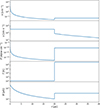 |
Fig. 2. Magnetohydrodynamic radial profiles describing the star cluster bubble. From top to bottom: Number density, plasma velocity, pressure, temperature, and magnetic field. |
 (45)
(45)
 (46)
(46)
 (47)
(47)
 (48)
(48)
as follows from Section 2.1. We set the total mass-loss rate to Ṁ = 2 × 10⁻⁴ M⊙/yr and the wind velocity to vw = 3 × 108 cm/s. The location of the termination shock is assumed to be at RTS = 20 pc in the adopted coordinate system, which corresponds to 21 pc from the centre of the star cluster. We note that here we ignored the outer part of the super bubble, assuming that they are of no importance in the context of maximum reachable energies of particles accelerated at the SNR shock. The spatial grid used in the hydrodynamic simulations extends to r = 60 pc with 524288 linearly spaced grid points. The evolution of the SNR shock throughout 7000 years in the classic case and 6000 years in the energetic case is shown on the left and right panels of Fig. 3, respectively. The abrupt drop of the shock velocity at around 2600 years in the classic case and just before 1000 years in the energetic case is associated with the shock reaching the termination shock. At this moment, a reflected shock is formed, travelling into the interior of the SNR. At some point in time, this type of shock bounces off the contact discontinuity inside the remnant and starts propagating towards the forward shock. At around 4000 years in the classic case and 1500 years in the energetic case, the reflected shock catches up with the forward shock giving it a boost. Once the shock starts propagating inside the downstream of the termination shock, the compression ratio decreases rapidly due to the high temperature of the medium there, leading to a small Mach number of the shock and a correspondingly steep spectrum exhibited by the accelerated particles.
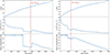 |
Fig. 3. Evolution of the shock radius, along with the velocity and compression ratio for the classic case on the left and energetic case on the right. The red vertical line indicates the time when the swept up by the shock mass becomes equal to the mass of the ejecta. |
4.1.2. Diffusion
For spatial diffusion, we investigated different regimes as described in Section 3. For pre-existing turbulence, we used expressions for the KOLM and KRAI diffusion (Eqs. (10) and (11)), applied to the whole simulation domain. The magnetic field is normalised to 10 μG in the wind at the location of the termination shock, which corresponds to 210 μG at the edge of the core of the stellar cluster. The spatial dependence of the magnetic field follows Eq. (4).
The possibility that a magnetic field can be efficiently self-generated can be studied based on the assumption of Bohm diffusion (BOHM; Eq. (23) with ηB = 1). To maximise the effect on the maximum energy and provide an upper limit to the particle acceleration process, we considered the case of a magnetic field amplified through the kinematic dynamo effect, following Eq. (37). The particle injection efficiency, η, is set at 10% of the ram pressure for this calculation. We note that in the performed simulations, the prescribed injection (see the next section) results in a time-dependent injection efficiency, but for the calculation of the amplified magnetic field, we froze the calculation at η = 0.1 to consider the most optimistic case that provides the highest value of the magnetic field. The amplified field acts only in the immediate upstream of the shock and exponentially decreases to the level of the background field on the length scale Δl = 0.05rs. The choice of 5% of the shock radius is consistent with the precursor length scale, ∼D(E)/vs2, at E ∼ 1 PeV. The background magnetic field in this scenario is assumed to be at the level of 10% of that assumed for the pre-existing turbulence, but this does not have any significant implications for the results. The amplified magnetic field δB upstream of the shock is shown in Fig. 4 as a function of time calculated for the cases of standard and energetic SN events. Initially, δB(t) was the same for both set-ups because δB ∝ vs/rs for the shock propagating in the wind zone of the bubble, but at later times, some differences arise because in the energetic case the SNR shock reaches the termination shock faster than in the standard case. In both cases, the first sharp increase in δB is associated with the SNR shock reaching the termination shock, where the upstream density increases by a factor of 4 and the second one is associated with the reflected shock catching up with the forward shock and giving it a boost. The Bohm-like diffusion is assumed to operate in the precursor, namely, up to 1.05rs, beyond which it transitions exponentially to the KOLM diffusion in the background field at two shock radii.
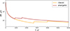 |
Fig. 4. Magnetic field in the immediate upstream of the shock amplified through the kinetic dynamo effect for the classic and energetic hydrodynamic set-ups. In both cases η = 0.1 is assumed. |
4.1.3. Particle acceleration
We used a kinetic approach to model the acceleration of CRs in the test-particle approximation. The time-dependent transport equation for the differential number density of cosmic rays, N(p, r, t), (Skilling 1975) is described by the following equation:
 (49)
(49)
where D denotes the spatial diffusion coefficient, u is the plasma velocity, ṗ represents energy losses, and Q is the source of thermal particles. The energy-loss term is relevant only for electrons, while here we only consider protons as accelerated particles. Equation (49) is solved using the FiPy-library (Guyer et al. 2009) in a frame co-moving with the shock. The radial coordinate is transformed according to (x − 1) = (x* − 1)3, where x = r/rs. This transformation guarantees a very fine resolution close to the shock for an equidistant binning of x*. The outer grid boundary extends to 65 shock radii upstream for xmax* = 5. Thus, all accelerated particles can be kept in the simulation domain.
Particle injection at the shock is described, for the sake of simplicity, through a thermal leakage model (Blasi et al. 2005),
 (50)
(50)
where χ is the injection efficiency parameter, nup and uup are the plasma number density and velocity in the upstream region, and pinj = ξpth is the injection momentum, defined as a multiple of the thermal momentum in the downstream plasma. In the performed simulations, we set ξ = 4 ensuring that the pressure of cosmic rays is always < 10% of the ram pressure, and hence cosmic rays are dynamically unimportant. The injection efficiency for the compression ratio of 4 is determined as
 (51)
(51)
4.2. Results
In Fig. 5, we show the evolution of the proton spectrum for the case of a standard SN explosion and different types of diffusion. Solid lines represent the total spectrum, while dashed and dash-dotted lines correspond to the downstream and upstream spectra, respectively. The vertical purple lines indicate the ‘knee’ energy of 3 PeV. It can be seen that the PeV energies are hard to reach in any of the considered scenarios. In the most optimistic case of Bohm diffusion, the maximum energy reaches at most a couple of hundred TeV. At around 2600 years, the SNR shock hits the termination shock and slows down considerably. Downstream of the termination shock, the gas is hot and the Mach number of the SNR shock decreases significantly. The compression ratio of the shock drops to almost 2.5, resulting in a very soft spectrum of freshly injected and accelerated particles with a spectral index of ∼3. Essentially, this means that the acceleration of freshly injected particles becomes irrelevant for the maximum energy at this stage. However, high-energy particles accelerated in earlier stages become compressed at the slowed down forward shock and may further gain some energy.
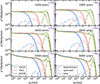 |
Fig. 5. Classic case for different turbulence models and ages. |
Roughly 4000 years after the explosion, the reflected shock reaches the forward shock and slightly energises it. However, this does not cause any visible effect of the spectrum of accelerated particles. Over time, particles injected after crossing the termination shock start dominating over the particles accelerated at earlier stages, which is evident from the soft spectrum at lower energies. It is worth keeping in mind that this conclusion depends on the adopted recipe for injection: for shocks with a Mach number of ∼2.5, the particle acceleration would be expected to shut down (Vink & Yamazaki 2014) and, as a result, this effect would disappear.
The mass of the swept-up material becomes equal to the mass of the ejecta shortly before 4000 years, meaning that at ∼5000−6000 years, the SNR is already deep in the Sedov-Taylor stage of the evolution and we would not expect further increase of the maximum energy.
In the energetic case, the situation is certainly more favourable. A higher shock velocity drives the acceleration of protons to a few hundred TeV, even in the case of the pre-existing turbulence with the Kraichnan diffusion coefficient. In Fig. 6, the evolution in time of the total particle spectrum is shown for such an energetic scenario, for the case of KRAI and BOHM diffusion. The only difference from the models presented in Fig. 5 is the explosion energy of the SN. The forward shock reaches the termination shock shortly before 1000 years, while the interaction with the reflected shock takes place at about 1500 years. The evolution of the spectra is similar to that in the classical case, with the main difference that higher maximum energies could be reached. Also, as a result of a higher shock velocity, the compression ratio of the shock stays high downstream of the termination shock (∼3.7 right after crossing the termination shock) for longer times and eventually drops to ∼3 only ∼5000 years after explosions, when the remnant is already very deep in the Sedov-Taylor stage. This increases the importance of particles injected after crossing the termination shock in the very-high-energy part of the spectrum and essentially prevents the formation of the pile-up feature in the downstream spectrum. It can be seen that in the case of the BOHM diffusion in the amplified field (as inferred for the kinetic dynamo effect), the spectrum of accelerated particles reaches PeV energies with a maximum energy saturating around the ‘knee’ energy of ∼3 PeV. It should be understood, however, that this result can only be achieved for rare, very energetic SN explosions and adopting the most optimistic assumptions on particle diffusion.
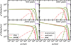 |
Fig. 6. Energetic case for KRAI and BOHM turbulence models for different ages. |
5. Summary and discussion
We numerically investigated the acceleration of cosmic rays at the shock of a SN exploded on the outskirts of a star cluster core, for a standard choice of the parameters of the explosion and an energetic case. The shock expands in the bubble excavated by the collective wind of the cluster and its dynamics is modified by this environment. Our analysis shows that the acceleration history does not differ sensibly from the case of an individual CC SNRs in the stellar wind bubble of the progenitor star and essentially faces the same difficulties when it comes to the acceleration to PeV energies. When the diffusion coefficient is dominated by the pre-existing magnetic turbulence, presumably present in the super bubble due to the interaction of winds of individual stars, it appears to be insufficient to warrant acceleration up to PeV energies. Only for energetic events with an explosion energy of 1052 erg is the pre-existing turbulence sufficient to accelerate particles to a few hundred TeV. The maximum energy for a standard SNR drops to values of a few tens of TeV.
The general conclusion is that acceleration to higher energies requires the self-generation of magnetic turbulence through streaming instabilities or other mechanisms, similarly to the case of isolated SNRs. When the explosion occurs in a super bubble, the conditions are adverse to the development of a non-resonant streaming instability, as previously pointed out by Morlino et al. (2021) and Blasi & Morlino (2023). Meanwhile resonant streaming instability seems insufficient to improve the odds of acceleration to PeV energies.
The most optimistic scenario that we consider here is the amplification of the background magnetic field through the kinetic dynamo effect, which could potentially provide conditions to enhance the magnetic field to larger values and lead to Bohm diffusion (Drury & Downes 2012; Beresnyak et al. 2009). In this borderline case, PeV energies can be reached only for very energetic, rare SNR explosions. This is not very different from the case of an isolated SNR.
Finally, it should be noted that while this manuscript was in revision, a new study was published proposing magnetic mirroring as an efficient mechanism to reach the level of Bohm diffusion in the presence of magnetic fluctuations at scales larger than the gyroradius (Bell et al. 2025). If this mechanism were indeed at work, the maximum energy would be pushed to PeV for pre-generated turbulence that we considered in the collective wind of the young compact stellar cluster. However, a similar environment is also expected for isolated young CC SNRs. So far, the observations do not show any evidence of acceleration to PeV energies in SNRs.
j = (n − 3)/(n − s), where n is the power-law index of the ejecta profile, which is commonly assumed to be 9 for CC SNRs and s is power-law index of the density profile, s = 2 for the wind zone.
Acknowledgments
IS acknowledges funding from Comunidad de Madrid through the Atracción de Talento “César Nombela” grant with reference number 2023-T1/TEC-29126. The work of PB has been partially funded by the European Union – Next Generation EU, through PRIN-MUR 2022TJW4EJ and by the European Union – NextGenerationEU under the MUR National Innovation Ecosystem grant ECS00000041 – VITALITY/ASTRA – CUP D13C21000430001, and by the research project TAsP (Theoretical Astroparticle Physics) funded by the Istituto Nazionale di Fisica Nucleare (INFN).
References
- Abeysekara, A. U., Albert, A., Alfaro, R., et al. 2021, Nat. Astron., 5, 465 [NASA ADS] [CrossRef] [Google Scholar]
- Ackermann, M., Ajello, M., Allafort, A., et al. 2013, Science, 339, 807 [NASA ADS] [CrossRef] [Google Scholar]
- Aharonian, F., Yang, R., & de Oña Wilhelmi, E. 2019, Nat. Astron., 3, 561 [Google Scholar]
- Aharonian, F., Ashkar, H., Backes, M., et al. 2022, A&A, 666, A124 [NASA ADS] [CrossRef] [EDP Sciences] [Google Scholar]
- Alfaro, R., Alvarez, C., Arteaga-Velázquez, J., et al. 2024, Nature, 634, 557 [Google Scholar]
- Amato, E., & Blasi, P. 2006, MNRAS, 371, 1251 [NASA ADS] [CrossRef] [Google Scholar]
- Ambrogi, L., Zanin, R., Casanova, S., et al. 2019, A&A, 623, A86 [NASA ADS] [CrossRef] [EDP Sciences] [Google Scholar]
- Bamba, A., Ueno, M., Nakajima, H., & Koyama, K. 2004, ApJ, 602, 257 [Google Scholar]
- Bell, A. R. 1978, MNRAS, 182, 147 [Google Scholar]
- Bell, A. R. 2004, MNRAS, 353, 550 [Google Scholar]
- Bell, A. R., Matthews, J. H., Taylor, A. M., & Giacinti, G. 2025, MNRAS, 539, 1236 [Google Scholar]
- Beresnyak, A., Jones, T. W., & Lazarian, A. 2009, ApJ, 707, 1541 [NASA ADS] [CrossRef] [Google Scholar]
- Binns, W. R., Wiedenbeck, M. E., Arnould, M., et al. 2008, New Astron. Rev., 52, 427 [CrossRef] [Google Scholar]
- Blasi, P., & Morlino, G. 2023, MNRAS, 523, 4015 [CrossRef] [Google Scholar]
- Blasi, P., Gabici, S., & Vannoni, G. 2005, MNRAS, 361, 907 [NASA ADS] [CrossRef] [Google Scholar]
- Brose, R., Telezhinsky, I., & Pohl, M. 2016, A&A, 593, A20 [NASA ADS] [CrossRef] [EDP Sciences] [Google Scholar]
- Brose, R., Sushch, I., Pohl, M., et al. 2019, A&A, 627, A166 [NASA ADS] [CrossRef] [EDP Sciences] [Google Scholar]
- Brose, R., Sushch, I., & Mackey, J. 2022, MNRAS, 516, 492 [NASA ADS] [CrossRef] [Google Scholar]
- Brose, R., Sushch, I., & Mackey, J. 2025, A&A, 699, A160 [NASA ADS] [CrossRef] [EDP Sciences] [Google Scholar]
- Clark, J. S., Ritchie, B. W., & Negueruela, I. 2020, A&A, 635, A187 [EDP Sciences] [Google Scholar]
- Cristofari, P., Blasi, P., & Amato, E. 2020a, Astropart. Phys., 123, 102492 [Google Scholar]
- Cristofari, P., Renaud, M., Marcowith, A., Dwarkadas, V. V., & Tatischeff, V. 2020b, MNRAS, 494, 2760 [NASA ADS] [CrossRef] [Google Scholar]
- Cristofari, P., Blasi, P., & Caprioli, D. 2021, A&A, 650, A62 [NASA ADS] [CrossRef] [EDP Sciences] [Google Scholar]
- Das, S., Brose, R., Meyer, D. M. A., et al. 2022, A&A, 661, A128 [NASA ADS] [CrossRef] [EDP Sciences] [Google Scholar]
- de Oña Wilhelmi, E., Sushch, I., Brose, R., et al. 2020, MNRAS, 497, 3581 [CrossRef] [Google Scholar]
- Diesing, R. 2023, ApJ, 958, 3 [NASA ADS] [CrossRef] [Google Scholar]
- Drury, L. O., & Downes, T. P. 2012, MNRAS, 427, 2308 [NASA ADS] [CrossRef] [Google Scholar]
- Giuliani, G., & AGILE Team 2011, Mem. Soc. Astron. Ital., 82, 747 [Google Scholar]
- Gupta, S., Nath, B. B., Sharma, P., & Eichler, D. 2020, MNRAS, 493, 3159 [CrossRef] [Google Scholar]
- Guyer, J. E., Wheeler, D., & Warren, J. A. 2009, Comput. Sci. Eng., 11, 6 [NASA ADS] [CrossRef] [Google Scholar]
- H.E.S.S. Collaboration (Abramowski, A., et al.) 2015, Science, 347, 406 [NASA ADS] [CrossRef] [Google Scholar]
- H.E.S.S. Collaboration (Aharonian, F., et al.) 2024, Science, 383, 402 [NASA ADS] [CrossRef] [Google Scholar]
- Härer, L. K., Reville, B., Hinton, J., Mohrmann, L., & Vieu, T. 2023, A&A, 671, A4 [NASA ADS] [CrossRef] [EDP Sciences] [Google Scholar]
- Härer, L., Vieu, T., & Reville, B. 2025, A&A, 698, A6 [NASA ADS] [CrossRef] [EDP Sciences] [Google Scholar]
- Inoue, T., Marcowith, A., Giacinti, G., Jan van Marle, A., & Nishino, S. 2021, ApJ, 922, 7 [NASA ADS] [CrossRef] [Google Scholar]
- Jogler, T., & Funk, S. 2016, ApJ, 816, 100 [Google Scholar]
- Joubaud, T., Grenier, I. A., Ballet, J., & Soler, J. D. 2019, A&A, 631, A52 [NASA ADS] [CrossRef] [EDP Sciences] [Google Scholar]
- Kavanagh, P. J., Vink, J., Sasaki, M., et al. 2019, A&A, 621, A138 [NASA ADS] [CrossRef] [EDP Sciences] [Google Scholar]
- Krumholz, M. R., McKee, C. F., & Bland-Hawthorn, J. 2019, ARA&A, 57, 227 [NASA ADS] [CrossRef] [Google Scholar]
- Lagage, P. O., & Cesarsky, C. J. 1983, A&A, 125, 249 [NASA ADS] [Google Scholar]
- LHAASO Collaboration 2024a, Sci. Bull., 69, 449 [NASA ADS] [CrossRef] [Google Scholar]
- LHAASO Collaboration 2024b, ArXiv e-prints [arXiv:2410.08988] [Google Scholar]
- Lingenfelter, R. E. 2018, Adv. Space Res., 62, 2750 [Google Scholar]
- Marcowith, A., Dwarkadas, V. V., Renaud, M., Tatischeff, V., & Giacinti, G. 2018, MNRAS, 479, 4470 [CrossRef] [Google Scholar]
- Mignone, A., Bodo, G., Massaglia, S., et al. 2007, ApJS, 170, 228 [Google Scholar]
- Morlino, G., Blasi, P., Peretti, E., & Cristofari, P. 2021, MNRAS, 504, 6096 [NASA ADS] [CrossRef] [Google Scholar]
- Parizot, E., Marcowith, A., van der Swaluw, E., Bykov, A. M., & Tatischeff, V. 2004, A&A, 424, 747 [NASA ADS] [CrossRef] [EDP Sciences] [Google Scholar]
- Portegies Zwart, S. F., McMillan, S. L. W., & Gieles, M. 2010, ARA&A, 48, 431 [NASA ADS] [CrossRef] [Google Scholar]
- Schure, K. M., & Bell, A. R. 2014, MNRAS, 437, 2802 [CrossRef] [Google Scholar]
- Skilling, J. 1975, MNRAS, 172, 557 [CrossRef] [Google Scholar]
- Sushch, I., Brose, R., & Pohl, M. 2018, A&A, 618, A155 [NASA ADS] [CrossRef] [EDP Sciences] [Google Scholar]
- Sushch, I., Brose, R., Pohl, M., Plotko, P., & Das, S. 2022, ApJ, 926, 140 [NASA ADS] [CrossRef] [Google Scholar]
- Telezhinsky, I., Dwarkadas, V. V., & Pohl, M. 2012, A&A, 541, A153 [NASA ADS] [CrossRef] [EDP Sciences] [Google Scholar]
- Telezhinsky, I., Dwarkadas, V. V., & Pohl, M. 2013, A&A, 552, A102 [NASA ADS] [CrossRef] [EDP Sciences] [Google Scholar]
- Vieu, T., & Reville, B. 2023, MNRAS, 519, 136 [Google Scholar]
- Vieu, T., Reville, B., & Aharonian, F. 2022a, MNRAS, 515, 2256 [NASA ADS] [CrossRef] [Google Scholar]
- Vieu, T., Gabici, S., Tatischeff, V., & Ravikularaman, S. 2022b, MNRAS, 512, 1275 [NASA ADS] [CrossRef] [Google Scholar]
- Vieu, T., Härer, L., & Reville, B. 2024a, MNRAS, 530, 4747 [Google Scholar]
- Vieu, T., Larkin, C. J. K., Härer, L., et al. 2024b, MNRAS, 532, 2174 [NASA ADS] [CrossRef] [Google Scholar]
- Vink, J. 2024, ArXiv e-prints [arXiv:2406.03555] [Google Scholar]
- Vink, J., & Yamazaki, R. 2014, ApJ, 780, 125 [Google Scholar]
- Wang, X., Yang, Y., Zhang, T., et al. 2005, ApJ, 626, L89 [Google Scholar]
- Weaver, R., McCray, R., Castor, J., Shapiro, P., & Moore, R. 1977, ApJ, 218, 377 [Google Scholar]
- Yamaguchi, H., Bamba, A., & Koyama, K. 2009, PASJ, 61, S175 [Google Scholar]
All Figures
|
Fig. 1. Schematic cartoon illustrating the considered scenario. Note: the ratios of the relevant length scales, i.e. the radius of the core, Rc, the radius of the termination shock, RTS, and the radius of the outer shock, Rb, do not reflect the real proportions. |
| In the text | |
|
Fig. 2. Magnetohydrodynamic radial profiles describing the star cluster bubble. From top to bottom: Number density, plasma velocity, pressure, temperature, and magnetic field. |
| In the text | |
|
Fig. 3. Evolution of the shock radius, along with the velocity and compression ratio for the classic case on the left and energetic case on the right. The red vertical line indicates the time when the swept up by the shock mass becomes equal to the mass of the ejecta. |
| In the text | |
|
Fig. 4. Magnetic field in the immediate upstream of the shock amplified through the kinetic dynamo effect for the classic and energetic hydrodynamic set-ups. In both cases η = 0.1 is assumed. |
| In the text | |
|
Fig. 5. Classic case for different turbulence models and ages. |
| In the text | |
|
Fig. 6. Energetic case for KRAI and BOHM turbulence models for different ages. |
| In the text | |
Current usage metrics show cumulative count of Article Views (full-text article views including HTML views, PDF and ePub downloads, according to the available data) and Abstracts Views on Vision4Press platform.
Data correspond to usage on the plateform after 2015. The current usage metrics is available 48-96 hours after online publication and is updated daily on week days.
Initial download of the metrics may take a while.