| Issue |
A&A
Volume 700, August 2025
|
|
|---|---|---|
| Article Number | A127 | |
| Number of page(s) | 9 | |
| Section | Stellar atmospheres | |
| DOI | https://doi.org/10.1051/0004-6361/202554267 | |
| Published online | 12 August 2025 | |
The peculiar composition of the Sun is not related to giant planets
1
Department of Physics and Astronomy, Uppsala University,
Box 516,
75120
Uppsala,
Sweden
2
Observatório Nacional/MCTIC, R. Gen. José Cristino,
77,
20921-400
Rio de Janeiro,
Brazil
3
Department of Physics and Astronomy, Aarhus University,
Ny Munkegade 120,
8000
Aarhus C,
Denmark
4
Department of Astronomy, Stockholm University,
AlbaNova University Center,
106 91
Stockholm,
Sweden
★ Corresponding authors: This email address is being protected from spambots. You need JavaScript enabled to view it.
Received:
25
February
2025
Accepted:
24
May
2025
Abstract
Highly differential spectroscopic studies have revealed that the Sun is deficient in refractory elements relative to solar twins. To investigate the role of giant planets on this signature, we present a high-precision abundance analysis of HARPS spectra for 50 F- and G-type stars spanning −0.4 ≲[Fe/H] ≲+0.5. There are 29 stars in the sample that host planets of masses ≳ 0.01 MJup.. We derived abundances for 19 elements and applied corrections to 14 of them for systematic errors associated with one dimensional (1D) model atmospheres, the assumption of local thermodynamic equilibrium (LTE), or both. We find that, among the solar twins in our sample, the Sun is Li poor in comparison to other stars at similar age, in agreement to previous studies. The sample shows a variety of trends in elemental abundances as a function of condensation temperature. We find a strong correlation in these trends with [Fe/H], with a marginally significant difference in the gradients for stars with and without giant planets detected, which increases after applying 3D and non-LTE corrections. Our overall results suggest that the peculiar composition of the Sun is primarily related to Galactic chemical evolution rather than the presence of giant planets.
Key words: line: formation / Sun: abundances / stars: abundances / stars: atmospheres / stars: late-type
© The Authors 2025
 Open Access article, published by EDP Sciences, under the terms of the Creative Commons Attribution License (https://creativecommons.org/licenses/by/4.0), which permits unrestricted use, distribution, and reproduction in any medium, provided the original work is properly cited.
This article is published in open access under the Subscribe to Open model. This email address is being protected from spambots. You need JavaScript enabled to view it. to support open access publication.
1 Introduction
The first planet discovered outside our Solar System was found around a pulsar by Wolszczan & Frail (1992); however, it was the discovery by Mayor & Queloz (1995) of a planet orbiting a solar-type star that marked the beginning of modern exoplanet research. Since then, more than 5000 planets have been detected around different types of stars1. A detailed review on the first exoplanets observed, the detection techniques and the stellar properties are shown in one of the first reviews on that topic by Udry & Santos (2007).
Stellar compositions offer a promising way to investigate and understand how those systems were formed. Stars and their planets form from the same cloud, thus, the elemental abundances of host stars put first-order constraints on the chemical composition of their planet (e.g. Thiabaud et al. 2015). Moreover, planet formation processes can cause small differences in stellar compositions relative to the protostellar nebula (e.g. Hühn & Bitsch 2023). Thus, elemental abundances of host stars also have the potential to shed light on how planets form.
Early studies found a positive correlation between stellar iron content [Fe/H]2 and the occurrence of massive planets (Santos et al. 2000; Fischer & Valenti 2005). The reason for these finds are still on debate, but possible explanations are either that a critical disc accretion rate to form planets correlates with metallicity (Liu et al. 2016) or that, instead of a planetary formation cause, we are observing a dynamical galactic effect due to stellar migration (Haywood 2009).
In this context, the study of other elements might shed more light on planetary formation. Works from Delgado Mena et al. (2010) and Adibekyan et al. (2012), among others, studied a large number of hosting planet stars and enriched the field with important material that was crucial to igniting the discussion surrounding planetary formation. Following this, several studies tried to link stellar composition and the occurrence of planets (Liu et al. 2021; Tautvaišienė et al. 2022, and references therein).
Notably, the work of Meléndez et al. (2009) concluded that the Sun is enriched in volatile elements and deficient in refractory elements compared to a sample of 11 solar twins (meaning stars with Δ Teff,☉ ≲ 100 K, Δ log g☉ ≲ 0.1 dex, and Δ[Fe/H]☉ ≲ 0.1 dex), none of which have confirmed planets to date. A similar result was found in the study of Bedell et al. (2018) with a broader sample of solar twins (about 80 stars). One possible explanation is that this material missing from the Sun was used in the formation of terrestrial planets.
In contrast to these results, González Hernández et al. (2010) and González Hernández et al. (2013) presented a similar study with a sample of approximately 100 and 60 F- and G-type stars (in a broader range of stellar parameters in comparison to solar twins: 5600 ≤ Teff(K) ≤ 6400, 4.0 ≤ log g ≤ 4.6 and −0.3 ≤ [Fe/H] ≤+0.5), respectively, and found no evidence correlating the volatile-to-refractory abundance ratio with the presence of rocky planets. More recently, Nibauer et al. (2021) analysed a large sample of 1700 solar-type stars with Δ Teff,☉ ≲ 195 K, Δ log g☉ ≲ 0.1 dex, and Δ[Fe/H]☉ ≲ 0.1 dex, using APOGEE data; they found two groups of stars regarding their content of refractory elements with the majority of the stars, which includes the Sun, belonging to the refractory poor group.
Several studies have suggested that the peculiar composition of the Sun could be related to planets. Booth & Owen (2020) argue that the Sun being refractory poor can be explained by the presence of giant planets, that might trap the dust outside their orbits and potentially cause the host star to be refractory-poor.
On the other hand, other works have highlighted the complications of this method when it comes to finding any signatures of planets around stars. Adibekyan et al. (2014) and Nissen (2015), which analysed solar-type stars, suggested that there is a dependence between the amount of refractory elements and stellar ages. Additionally, Swastik et al. (2022) compiled chemical abundances for planet-hosting stars in distinct evolutionary states and concluded that observed abundance trends with planet mass are a consequence of the chemical evolution of our Galaxy. However, Adibekyan et al. (2016), who also found a correlation of refractory elements with stellar ages, suggested that the signature of the chemical evolution of the Galaxy on the amount of refractory elements in hosting planet stars might be erased for stars with similar ages.
Finally, alternative scenarios involving processes in the protoplanetary disc could also explain these abundance patterns, such as a self-dust cleansing caused by radiation of the protoSun (Gustafsson 2018). Planet engulfments could also cause an excess of refractory elements in the stellar atmosphere (Spina et al. 2021; Liu et al. 2024), as shown in the analysis of wide binary systems presented in Oh et al. (2018) and Nagar et al. (2020), for example.
In an attempt to shed light on this topic, we present a highprecision analysis of 19 elements in high-resolution spectra of 50 F- and G-type stars with and without giant planets (Sect. 2). To improve the accuracy of the analysis, we applied corrections to the 1D LTE abundances for 14 elements. We inspected the resulting trends in abundances with condensation temperature (Sect. 3) and find a strong correlation with [Fe/H], suggesting that giant planets may at most impart only a second-order effect on the stellar compositions (Sect. 4).
2 Method
The sample consists of 50 F- and G-type stars observed with the HARPS spectrograph (Mayor et al. 2003) at the 3.6 m ESO telescope. These objects were previously presented in Nissen et al. (2014) and Amarsi et al. (2019) and can be found in the ESO Science Archive3. The spectra have high resolution and good signal-to-noise ratios (R = 115 000 and S/N ≳ 200). Our study was performed by analysing the red HARPS spectra, which have a wavelength coverage from 5330 to 6910Å. Additionally, the solar HARPS spectrum was obtained by observing the reflected sunlight in the Vesta asteroid. Twenty nine stars in our sample host at least one exoplanet (58% of the sample), and the exoplanet distances go from 0.03 to 13.18 AU with 0.016 ≤ M sin i ≤ 16.64 Mjup..
Photometric effective temperatures (Teff) were calculated by Nissen et al. (2014), while microturbulence velocities (ξturb.) and iron abundance ([Fe/H]) are from Amarsi et al. (2019). With the aid of the q2 code (Ramírez et al. 2014), we updated the surface gravity (log g) values using the updated magnitudes and parallaxes from GAIA DR3 (Gaia Collaboration 2023; Babusiaux et al. 2023) and Yonsei-Yale isochrones (Yi et al. 2001; Kim et al. 2002). We note that the mean difference in log g from the former values is of about −0.01 dex.
The sample consists of stars with Teff from 5450 to 5950 K (with a typical statistical error of 30 K), log g between 3.9 and 4.6 dex (typical statistical error of ± 0.02 dex), −0.4 ≤[Fe/H] ≤ 0.5 (typical statistical error of ± 0.007 dex), and ξturb. between 0.7 and 1.5 km s−1 (typical statistical error of ± 0.06 km s−1). The systematic errors are larger, as discussed in Casagrande et al. (2010) and Nissen et al. (2014), and can be around 65 K for Teff and 0.10 dex for log g.
We calculated the 1D LTE abundances of Na I, Mg I, Al I, Si I, S I, Ca I, Sc I and Sc II, Ti I and Ti II, V I, Cr I and Cr II, Mn I, Co I, Ni I, Cu I, and Zn I, measuring the equivalent widths with IRAF (Tody 1986, 1993) and applying a differential line-by-line analysis (Bedell et al. 2014) using the 2019 version of the 1D radiative transfer code MOOG (Sneden 1973), q2, and the grid of standard MARCS model atmospheres (Gustafsson et al. 2008). The line list used for these measurements was adapted from Bedell et al. (2018), with a hyperfine structure for S I from Civiš et al. (2024), V I, Mn I, Co I from Bedell et al. (2018), and Cu I from Shi et al. (2014). We also determined Li abundances for all stars through spectral synthesis in the same way as in Carlos et al. (2019). We adopted Teff=5772 K and log g=4.44 dex for the Sun. For our 1D LTE and 1D non-LTE results, we took ξturb.= 1.2 km s−1 for the disc-integrated solar flux (Takeda 2022).
We considered 3D non-LTE effects for several elements. First, for Li we adopted the 3D non-LTE versus 1D LTE abundance corrections from Wang et al. (2021). We note that these corrections are strictly based on ξturb. = 1 km s−1, and so we were careful to adopt that value of ξturb. in our 1D LTE analysis of Li. For C and O, we adopted the 3D non-LTE abundances given in Amarsi et al. (2019); for Fe we adopted the 3D LTE ones in that same paper, noting that the iron abundances are based on Fe II lines that show negligible departures from 3D LTE in solar-metallicity FGK-type stars (e.g. Amarsi et al. 2022). For Mg, we adopted the 3D non-LTE abundances given in Matsuno et al. (2024), which are based on 3D non-LTE abundance corrections to the 1D LTE abundances derived in the present study. For Na, we extended the 3D non-LTE grid presented in Canocchi et al. (2024) and determined absolute 3D non-LTE versus 1D LTE corrections. These were interpolated onto our stellar and solar parameters and subtracted to obtain differential 3D non-LTE versus 1D LTE corrections. These calculations will be described fully in a forthcoming work (Canocchi et al., in prep.). All of these 3D non-LTE abundances are based on the code Balder (Amarsi et al. 2018, 2022), which originates from Multi3D (Leenaarts & Carlsson 2009), with several modifications, in particular to the equation of state and background opacities.
For Si, S, and Ca, we calculated new 1D non-LTE corrections with the code Balder. The calculations were performed on a grid of MARCS model atmospheres as described in Amarsi et al. (2020), for five different values of abundance, A(X), and three different values of ξturb.. This allowed us to calculate a grid of abundance corrections, which we then interpolated onto our stellar parameters and 1D LTE abundances using cubic splines. The exact same approach was adopted for the Sun, and thereby differential 1D non-LTE abundance corrections were applied on [X/H]. The model atoms for Si originate from Amarsi & Asplund (2017), with small updates to the hydrogen collisions and complexity as described in Nissen et al. (2024), while the model atom for Ca originates from Asplund et al. (2021) and has been used in Lagae et al. (2023). For S, we updated the model atom recently employed in Kochukhov et al. (2024), in particular to include electron collision data from OpenADAS (Summers & O'Mullane 2011). In any case, our calculations and tests indicate that the differential abundance corrections are negligible, at least for the present sample of stars and for the weak subordinate S lines used in this work. A full description of the model and benchmarking on the Sun will be presented in a forthcoming work (Amarsi et al., in prep.).
In addition, we corrected our abundances of Al, Ti, Cr, Mn, and Co for 1D non-LTE departures. For Al, we employed the scripts provided by Nordlander & Lind (2017). For the other elements we used the MPIA non-LTE database (Kovalev et al. 2018), which are based on older model atoms from Bergemann (2011), Bergemann & Cescutti (2010), Bergemann & Gehren (2008), and Bergemann et al. (2010) that adopt the Drawin recipe for inelastic collisions with neutral hydrogen (Steenbock & Holweger 1984; Lambert 1993). Lines of Sc I, Sc II, V I, Ni I, Cu I, and Zn I were treated in 1D LTE.
To evaluate any systematics from the choice of model atmospheres, we repeated our 1D LTE analysis with ATLAS models (Castelli & Kurucz 2003), for elements from Na to Zn. Ultimately, in a differential analysis the abundance differences between the calculations with MARCS or ATLAS are negligible within the errors. The average difference in abundance is about −0.005 dex, and the maximum difference is about ± 0.01 dex for the most metal-poor stars in our sample ([Fe/H] ≤−0.20). While Delgado Mena et al. (2021) found a significant difference in abundances of C and O when comparing ATLAS and MARCS models, these elements are here adopted from the detailed 3D non-LTE study of Amarsi et al. (2019).
The final abundance errors were estimated by considering the stellar-parameter uncertainties and the statistical error associated with the abundances inferred from line-to-line scatter. For the specific cases of Mg, Cu, and Zn, only one line was available. Then, those individual lines were measured three times repeatedly with slightly different continuum positions so as to estimate a statistical uncertainty. The stellar parameters and planetary information are in Table 1 and LTE and non-LTE abundances and the respective errors are presented in Table 2; both are available at the CDS.
Stellar identification, effective temperature (K), microturbulence velocity (km s−1), surface gravity (dex), [Fe/H], age (Gyr) and respective errors, number of planets detected, and planetary-system mass (Mjup.) adopted in this work.
Stellar identification and stellar abundances in 1D LTE, 1D non-LTE, and 3D non-LTE, when available, and their respective errors.
3 Results
3.1 Lithium
Because Li burns at low temperatures (2.5 × 10⁶ K) below the convective zone of solar-type stars, its abundance is highly sensitive to stellar parameters and age (Carlos et al. 2016). In addition, over the past two decades works in the literature have debated a possible connection between Li depletion and the presence of planets. For instance, the work of Israelian et al. (2009), followed by the more refined analysis of Delgado Mena et al. (2014), concluded that the Li depletion is also related to the presence of planets, even if as a secondary effect. Other studies, such as Ghezzi et al. (2010) and Llorente de Andrés et al. (2024), also discuss the composition of Li on hosting planet stars. On top of that, the work of Spina et al. (2021) claimed that a planet engulfment event can cause an excess of Li in the stellar atmosphere.
With all these considerations, it is hard to assess only the (giant) planet effect on Li abundances in solar type stars with a broader range of stellar parameters, in comparison to, for example, solar twins (Rathsam et al. 2023). Nonetheless, we present our 3D non-LTE Li abundances versus Teff divided into stars with or without giant planets detected in Figure 1; there is no noticeable distinction between the two sub-samples. The typical scatter for a given Teff is of about 0.34 dex, which is the same for 1D LTE abundances and probably caused by other issues (such as age, metallicity, etc.). Moreover, the Sun shows a reasonable Li abundance in comparison to other solar-type stars at given Teff and age; however, if we consider only the solar twins in our sample the Sun is the most Li poor for its age (in agreement with Carlos et al. 2019).
From Figure 1, it is also possible to note two outliers that present a higher Li content for their Teff, namely HD 1237 (Teff= 5507 K and A(Li)=2.03 dex) and HD 114613(Teff=5700 K. and A(Li)=2.53 dex). To assess whether this discrepancy in the Li abundances was a result of their stellar convective envelopes being smaller than expected for their masses and [Fe/H] (hence less Li destruction), we calculated the mass of the convective envelope for all stars in our sample by interpolating the values from the YaPSI grid of isochrones (Spada et al. 2017). From those values we can speculate that the HD 114613 higher content of Li in comparison to stars at similar Teff might be due to its shallower convective envelope in comparison to other stars at similar Teff. On the contrary, HD 1237 has a convective envelope mass comparable to other stars at the same Teff; thus, their higher Li content might be due to planet engulfment (as discussed in Carlos et al. 2019; Spina et al. 2021; Sevilla et al. 2022).
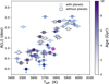 |
Fig. 1 Absolute Li abundance versus Teff. Stars with giant planets are shown in blue circles and stars without giant planets detected are presented by black squares; the Sun is shown by its usual symbol in purple. The data are colour-coded by age. |
3.2 Stellar abundances and comparison with solar twins
In this section, we discuss all the other stellar abundances adopted in this work, and what we call the best possible determination. When available, we first consider 3D non-LTE as the best option, followed by 3D LTE, then 1D non-LTE, and finally 1D LTE.
For details on how the 3D (non-)LTE analyses of C, O, Mg, and Fe affect the data, we refer the reader to Amarsi et al. (2019) and Matsuno et al. (2024). For the remaining elements, the typical solar-differential corrections vary from −0.0248 dex (Mn I) to +0.0155 dex(Cr I). For most elements, the 1D or 3D non-LTE corrections tend to diminish the line-by-line scatter, including for Na I from Canocchi et al. (in prep.); Al I from Nordlander & Lind (2017); and Si I, S I, and Ca I calculated in this work. However, this was not the case for Mn I based on corrections from Bergemann & Gehren (2008). Similarly, the 1D non-LTE corrections for the Ti I and Ti II from Bergemann (2011), worsened the line-by-line scatter and ionisation equilibrium. This may reflect the necessity for full 3D non-LTE analyses, as suggested by Mallinson et al. (2024) via their analysis of Ti in metal poor dwarfs in 1D non-LTE and 3D LTE. Furthermore, 20% of the stars in our sample have their line-by-line scatter increased by as much as 0.035 dex for Cr I, when applying non-LTE corrections from Bergemann & Cescutti (2010), strongly affecting their final uncertainties. The Co I line-by-line scatter in 1D LTE was similar to that after the 1D non-LTE corrections from Bergemann et al. (2010).
Figure 2 shows [C/Fe], [O/Fe], [Na/Fe], [Mg/Fe], [Al/Fe], [Si/Fe], [S/Fe], [Ca/Fe], [Sc/Fe], [Ti/Fe], [V/Fe], [Cr/Fe], [Cu/Fe], and [Zn/Fe] as a function of [Fe/H] for all stars in our sample (with and without giant planets detected) in comparison with the abundances of thin-disc solar twins from Bedell et al. (2018); our method of analysis for a given element is highlighted in the bottom left of each panel, with [Fe/H] always in 3D LTE. The Sc, Ti, and Cr abundances adopted from now on were calculated as the weighted average from Sc I and Sc II, Ti I and Ti II, and Cr I and Cr II, respectively.
The abundances determined in our work are similar to those from Bedell et al. (2018). This good agreement is no surprise since we employed a similar method of analysis and adopted a similar line list. The main difference remains in the fact that Bedell et al. (2018) relied predominantly on a 1D LTE analysis. O is the only exception where they adopted a 1D non-LTE analysis of the OI 777 nm lines with corrections from Ramírez et al. (2013). Here, our O comes from a 3D non-LTE analysis of the same lines as Amarsi et al. (2019). There appears to be a systematic difference between the two studies such that at solar metallicity the mean [O/Fe] is around 0.04 dex higher in Bedell et al. (2018) than in Amarsi et al. (2019). This means that the Sun is slightly oxygen-poor compared to solar twins according to the former study.
It is interesting to note that our [Ca/Fe] decreases with [Fe/H], while that of Bedell et al. (2018) shows a flat distribution with [Fe/H]. Other works, such as Sun et al. (2025) and the GALAH DR4 (Buder et al. 2024), also suggest a tendency of decreasing [Ca/Fe] with [Fe/H].
Moreover, a more careful look at the [Mn/Fe] distributions shows that the Bedell et al. (2018) values increase with [Fe/H], which is not the case for our data. This somewhat flat distribution in our data only appears after the 1D non-LTE correction (as also found in Bergemann & Gehren 2008). Our 1D LTE [Mn/Fe] also increases with [Fe/H]. It is important to note that even after nonLTE corrections the [Mn/Fe] abundances from the GALAH DR3 and GALAH DR4 also increase with [Fe/H] (Amarsi et al. 2020; Buder et al. 2024).
For a detailed comparison between our results and those of Bedell et al. (2018), we analysed the scatter in the [X/Fe] distributions in the metallicity interval from −0.10 to +0.10 dex. The star-to-star scatter was calculated in bins of 0.05 dex in [Fe/H], and the following values are the weighted mean for each element.
Even though our sample has a broader range in Teff, log g, and ξturb., the star-by-star scatter in our sample is comparable with the scatter from Bedell et al. (2018); in some cases, it is smaller. Our typical scatter varies from 0.014 dex ([Si/Fe]) to 0.055 dex ([S/Fe]), while the typical scatter in the Bedell et al. (2018) data goes from 0.013 dex([Cr/Fe]) to 0.045 dex([Cu/Fe]). In general, we present smaller star-by-star scatter for [O/Fe], [Mg/Fe], [Si/Fe], [Co/Fe], and [Cu/Fe]; greater star-by-star scatter for [C/Fe], [Na/Fe], [S/Fe], [Ca/Fe], [Sc/Fe], [Ti/Fe], [V/Fe], [Cr/Fe], [Mn/Fe], and [Zn/Fe]; and similar star-by-star scatter for [Al/Fe] and [Ni/Fe].
3.3 Condensation temperature trends
Figure 3 presents [X/H] as a function of elemental condensation temperatures (Tcond, from Lodders 2003) for two stars in our sample. For comparison, we plot both the 1D LTE (black) and non-LTE (red) 1D or 3D abundances. In order to assess the behaviour of those abundances' distributions for each star, we decided to perform two linear fits: one considering all abundances in 1D LTE, and the other considering the “best” available abundances for a given element, namely 3D non-LTE, 3D LTE, 1D non-LTE, or 1D LTE as applicable. The best linear fit for elements with Tcond ≥ 900 K was retrieved considering the maximum likelihood estimation. The choice to only consider elements with Tcond ≥ 900 K for the linear fits was discussed in detail in Bedell et al. (2018). The uncertainties were estimated via a Markov chain Monte Carlo (MCMC) method using the python package emcee (Foreman-Mackey et al. 2013).
The Tcond slopes derived in this way for each case and their respective errors are present in Table 3 at the CDS. We note that the two linear fit cases (1D LTE and best abundances) are compatible to within one sigma for every star. From now on, the discussion about the Tcond slopes are restricted to those considering the best set of abundances.
In Figure 4, we present the Tcond slopes for stars with and without giant planets, versus stellar parameters Teff (top left), log g (top right), ξturb. (bottom left), and [Fe/H] (bottom right). No evident correlation with Teff, log g, and ξturb. was found. On the other hand, a strong anti-correlation with [Fe/H] is seen in the bottom right panel of Figure 4. Once more, the best linear fits, for hosting giant planets stars (blue dashed line) and stars without detected giant planets (black dot-dashed line), were retrieved considering the maximum likelihood estimation with the uncertainties computed via an MCMC method. This time, we took into account the Tcond slopes and their errors and [Fe/H]. The blue and black dashed area represents the 1.5 σ interval for each linear fit.
Moreover, from the bottom right panel of Figure 4, it is noticeable that the Sun is marginally poorer from a refractory perspective than stars at similar metallicities; that is, a 1.7 standard deviation below the stars distributed within −0.05 ≤ [Fe/H] ≤+0.05. To test if the fact that the Sun being refractorypoor is due to systematic errors in the stellar parameters, we perturbed Teff, log g, and ξturb. until the stars in our sample were shifted down so that the Sun was the middle of the distribution. No significant changes in this distribution were found for Teff and log g when using perturbations of up to 300 K and 0.3 dex. For ξturb., a difference of 1 km s−1 was needed for the Sun to be considered typical in this sample.
The Tcond slopes versus [Fe/H] trend presumably reflects Galactic chemical evolution. To gain a deeper understanding of it, we repeated the steps above, but separated elements into their two major production sites (Nomoto et al. 2013): first, considering only alpha elements (O, Mg, Si, S, Ca, and Ti); second, considering non-alpha elements. Figure 5 presents a comparison between the different Tcond slopes as a function of [Fe/H], for stars both with and without giant planets detected. The alpha and non-alpha slopes typically differ in 0.41 × 10⁻⁴ dex K−1 and 0.93 × 10⁻⁴ dex K−1 for stars with and without giant planets detected, respectively. The slopes for stars with or without giant planets detected differ typically in 0.29 × 10⁻⁴ dex K−1 and −0.07 × 10⁻⁴ dex K−1 when we consider only alpha elements or only non-alpha elements, respectively. Although a variation was found, the difference in the Tcond slopes for alpha or nonalpha elements, and also for stars with or without giant planets detected, are compatible in 1 σ for most [Fe/H] values.
The chemical evolution of our Galaxy may also impart a signature on the behaviour of Tcond slopes versus planetary system mass and planet distance. These are shown in the top left and right panels of Figure 6, respectively. A weak anti-correlation was found for the Tcond slope versus planetary system mass and planet distances (Spearman coefficient equal to −0.60 and −0.58, respectively), where the stellar systems with more massive and distant planets present Tcond slopes lower than 1.0 × 10⁻⁴ dex K−1. This is in agreement with Yun et al. (2024), who analysed thin-disc stars' APOGEE DR17 spectra and also found that for giant planets the Tcond slopes were negative for most of the stars. Interestingly, this anti-correlation goes away in our study in the lower panels of Figure 6, which replace the Tcond slope with the Δ Tcond slope, given by the Tcond,obs slope – the Tcond,fit slope; in other words, this is done by subtracting the linear fit as a function of [Fe/H] (blue dashed line in Figure 4). We also notice that in these plots the Sun is refractory-poor when compared to other solar-like stars.
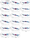 |
Fig. 2 [X/Fe] versus [Fe/H] for stars in our sample with (blue circles) and without (black squares) giant planets detected, in comparison with thin-disc solar twins (pink stars) from Bedell et al. (2018). |
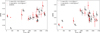 |
Fig. 3 [X/H] as function of elemental condensation temperatures for stars HD 196761 (without detected giant planets, left panel) and HD 82943 (with two giant planets detected, right panel). Black circles represent elemental abundances in 1D LTE, while red circles show 1D non-LTE, 3D LTE, or 3D non-LTE (when available). The best fit including only the refractory elements with Tcond ≥ 900 K are represented by the solid grey (1D non-LTE) and red dashed (1D and 3D non-LTE) lines. |
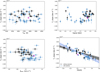 |
Fig. 4 Condensation temperature slopes versus stellar parameters Teff (top left panel), log g (top right panel), ξturb. (bottom left panel), and [Fe/H] (bottom right panel). Stars with giant planets are shown in blue, and stars without giant planets detected are presented by black squares. The Sun is shown by its usual symbol in purple. |
Stellar identification, Tcond slopes (dex K−1) using the ‘best’ set of abundances and the 1D LTE ones, and the respective errors.
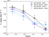 |
Fig. 5 Tcond slopes only considering α-elements (dashed line) or non α-elements (dot-dashed line) as a function of [Fe/H] for stars with (dark and light blue circles) and without (grey and black squares) giant planets. |
4 Discussion and conclusions
There is a strong correlation between the Tcond slopes and [Fe/H] shown in Figure 4. This suggests that studies of abundance trends with condensation temperature are strongly affected by the chemical evolution of our Galaxy. The work of Adibekyan et al. (2014) analysed solar analogues and found a dependence between Tcond slopes and stellar age and suggested that the Tcond slopes are affected by the chemical evolution of our Galaxy, although they were not able to find any relation between the Tcond slope and [Fe/H]. More recently, Sun et al. (2025) found a correlation between the Tcond slope and [Fe/H] for stars with −0.4 ≲ [Fe/H] ≲+0.4, but no significant correlations were found for solar twins. We also found that the corrections to the 1D LTE abundances only lightly affect the Tcond slopes, as discussed in Sect. 3.3. Thus, the Tcond slope versus [Fe/H] plot with only 1D LTE abundances is very similar to the one considering non-LTE corrections, shown in the bottom right panel of Figure 4. This shows that the correlation of the Tcond slopes and [Fe/H] seen is this figure is not related to departures from 1D LTE.
Giant planets may impart a second-order effect on abundance trends with condensation temperature, given the marginally significant differences in the linear correlations of the Tcond slope versus [Fe/H] for the two populations of stars (with and without giant planets); these are overplotted in Figure 4. Increasing the sample of high resolution spectra of stars with and without planets would help us make a stronger statement regarding the differences between the two linear fits in this panel. Moreover, improving the accuracy of abundance analyses appears to be important. The difference between the slopes for stars with and without giant planets is slightly affected by the corrections to 1D LTE abundances. The difference is increased from 1 σ in 1D LTE to 1.5σ when 3D or non-LTE corrections are applied.
Finally, the Sun is slightly refractory-poor when compared to other stars of similar [Fe/H](−0.05 ≲[Fe/H] ≲+0.05), with marginal significance levels. This is in agreement with analyses of solar twins (Meléndez et al. 2009; Bedell et al. 2018) and solar analogues (Rampalli et al. 2024). Nine stars are within this [Fe/H] interval (including the Sun), four of which have had giant planets detected. In this region, there is no obvious difference in the correlation of the Tcond slope versus [Fe/H] (Figure 4) for stars with and without giant planets. This suggests that the Sun is peculiar for some other reason than the presence and influence of giant planets.
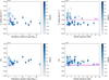 |
Fig. 6 Top panels: Tcond slopes versus planetary system mass (top left) and planet distance (top right). Lower panels: ΔTcond slopes versus planetary system mass (bottom left) and planet distance (bottom right). The Sun is shown by its usual symbol (left panels) or a dashed line (right panels), in purple. |
Data availability
Tables 1–3 are available at the CDS via https://cdsarc.cds.unistra.fr/viz-bin/cat/J/A+A/700/A127
Acknowledgements
MC and GC acknowledges funds from the Knut and Alice Wallenberg foundation. This work is a part of the project “Probing chargeand mass-transfer reactions on the atomic level” supported by the Knut and Alice Wallenberg Foundation (2018.0028). AMA acknowledges support from the Swedish Research Council (VR 2020-03940), the Crafoord Foundation via the Royal Swedish Academy of Sciences (CR 2024-0015), and from the European Union's Horizon Europe research and innovation programme under grant agreement No. 101079231 (EXOHOST). This research was supported by computational resources provided by the Australian Government through the National Computational Infrastructure (NCI) under the National Computational Merit Allocation Scheme and the ANU Merit Allocation Scheme (project y89). This work presents results from the European Space Agency (ESA) space mission Gaia. Gaia data are being processed by the Gaia Data Processing and Analysis Consortium (DPAC). Funding for the DPAC is provided by national institutions, in particular the institutions participating in the Gaia MultiLateral Agreement (MLA). The Gaia mission website is https://www.cosmos.esa.int/gaia. The Gaia archive website is https://archives.esac.esa.int/gaia. This research has made use of the NASA Exoplanet Archive, which is operated by the California Institute of Technology, under contract with the National Aeronautics and Space Administration under the Exoplanet Exploration Program.
References
- Adibekyan, V. Z., Sousa, S. G., Santos, N. C., et al. 2012, A&A, 545, A32 [NASA ADS] [CrossRef] [EDP Sciences] [Google Scholar]
- Adibekyan, V. Z., González Hernández, J. I., Delgado Mena, E., et al. 2014, A&A, 564, L15 [NASA ADS] [CrossRef] [EDP Sciences] [Google Scholar]
- Adibekyan, V., Delgado-Mena, E., Figueira, P., et al. 2016, A&A, 592, A87 [NASA ADS] [CrossRef] [EDP Sciences] [Google Scholar]
- Amarsi, A. M., & Asplund, M., 2017, MNRAS, 464, 264 [Google Scholar]
- Amarsi, A. M., Nordlander, T., Barklem, P. S., et al. 2018, A&A, 615, A139 [NASA ADS] [CrossRef] [EDP Sciences] [Google Scholar]
- Amarsi, A. M., Nissen, P. E., & Skúladóttir, Á. 2019, A&A, 630, A104 [NASA ADS] [CrossRef] [EDP Sciences] [Google Scholar]
- Amarsi, A. M., Lind, K., Osorio, Y., et al. 2020, A&A, 642, A62 [EDP Sciences] [Google Scholar]
- Amarsi, A. M., Liljegren, S., & Nissen, P. E., 2022, A&A, 668, A68 [NASA ADS] [CrossRef] [EDP Sciences] [Google Scholar]
- Asplund, M., Amarsi, A. M., & Grevesse, N., 2021, A&A, 653, A141 [NASA ADS] [CrossRef] [EDP Sciences] [Google Scholar]
- Babusiaux, C., Fabricius, C., Khanna, S., et al. 2023, A&A, 674, A32 [NASA ADS] [CrossRef] [EDP Sciences] [Google Scholar]
- Bedell, M., Meléndez, J., Bean, J. L., et al. 2014, ApJ, 795, 23 [Google Scholar]
- Bedell, M., Bean, J. L., Meléndez, J., et al. 2018, ApJ, 865, 68 [Google Scholar]
- Bergemann, M., 2011, MNRAS, 413, 2184 [NASA ADS] [CrossRef] [Google Scholar]
- Bergemann, M., & Gehren, T., 2008, A&A, 492, 823 [NASA ADS] [CrossRef] [EDP Sciences] [Google Scholar]
- Bergemann, M., & Cescutti, G., 2010, A&A, 522, A9 [NASA ADS] [CrossRef] [EDP Sciences] [Google Scholar]
- Bergemann, M., Pickering, J. C., & Gehren, T., 2010, MNRAS, 401, 1334 [CrossRef] [Google Scholar]
- Booth, R. A., & Owen, J. E., 2020, MNRAS, 493, 5079 [NASA ADS] [CrossRef] [Google Scholar]
- Buder, S., Kos, J., Wang, E. X., et al. 2024, PASA, 42, e051 [Google Scholar]
- Canocchi, G., Morello, G., Lind, K., et al. 2024, A&A, 692, A43 [NASA ADS] [CrossRef] [EDP Sciences] [Google Scholar]
- Carlos, M., Nissen, P. E., & Meléndez, J., 2016, A&A, 587, A100 [NASA ADS] [CrossRef] [EDP Sciences] [Google Scholar]
- Carlos, M., Meléndez, J., Spina, L., et al. 2019, MNRAS, 485, 4052 [Google Scholar]
- Casagrande, L., Ramírez, I., Meléndez, J., Bessell, M., & Asplund, M., 2010, A&A, 512, A54 [NASA ADS] [CrossRef] [EDP Sciences] [Google Scholar]
- Castelli, F., & Kurucz, R. L., 2003, in Modelling of Stellar Atmospheres, 210, eds. N. Piskunov, W. W. Weiss, & D. F. Gray, A20 [NASA ADS] [Google Scholar]
- Civiš, S., Kramida, A., Zanozina, E. M., et al. 2024, ApJS, 274, 32 [Google Scholar]
- Delgado Mena, E., Israelian, G., González Hernández, J. I., et al. 2010, ApJ, 725, 2349 [NASA ADS] [CrossRef] [Google Scholar]
- Delgado Mena, E., Israelian, G., González Hernández, J. I., et al. 2014, A&A, 562, A92 [NASA ADS] [CrossRef] [EDP Sciences] [Google Scholar]
- Delgado Mena, E., Adibekyan, V., Santos, N. C., et al. 2021, A&A, 655, A99 [NASA ADS] [CrossRef] [EDP Sciences] [Google Scholar]
- Fischer, D. A., & Valenti, J., 2005, ApJ, 622, 1102 [NASA ADS] [CrossRef] [Google Scholar]
- Foreman-Mackey, D., Hogg, D. W., Lang, D., & Goodman, J., 2013, PASP, 125, 306 [Google Scholar]
- Gaia Collaboration (Vallenari, A., et al.,) 2023, A&A, 674, A1 [NASA ADS] [CrossRef] [EDP Sciences] [Google Scholar]
- Ghezzi, L., Cunha, K., Smith, V. V., & de la Reza, R., 2010, ApJ, 724, 154 [NASA ADS] [CrossRef] [Google Scholar]
- González Hernández, J. I., Israelian, G., Santos, N. C., et al. 2010, ApJ, 720, 1592 [CrossRef] [Google Scholar]
- González Hernández, J. I., Delgado-Mena, E., Sousa, S. G., et al. 2013, A&A, 552, A6 [NASA ADS] [CrossRef] [EDP Sciences] [Google Scholar]
- Gustafsson, B., 2018, A&A, 620, A53 [NASA ADS] [CrossRef] [EDP Sciences] [Google Scholar]
- Gustafsson, B., Edvardsson, B., Eriksson, K., et al. 2008, A&A, 486, 951 [NASA ADS] [CrossRef] [EDP Sciences] [Google Scholar]
- Haywood, M., 2009, ApJ, 698, L1 [NASA ADS] [CrossRef] [Google Scholar]
- Hühn, L. A., & Bitsch, B., 2023, A&A, 676, A87 [NASA ADS] [CrossRef] [EDP Sciences] [Google Scholar]
- Israelian, G., Delgado Mena, E., Santos, N. C., et al. 2009, Nature, 462, 189 [NASA ADS] [CrossRef] [Google Scholar]
- Kim, Y.-C., Demarque, P., Yi, S. K., & Alexander, D. R., 2002, ApJS, 143, 499 [Google Scholar]
- Kochukhov, O., Amarsi, A. M., Lavail, A., et al. 2024, A&A, 689, A36 [NASA ADS] [CrossRef] [EDP Sciences] [Google Scholar]
- Kovalev, M., Brinkmann, S., Bergemann, M., & MPIA IT-department 2018 [Google Scholar]
- NLTE MPIA web server, [Online]. Available: http://nlte.mpia.de [Google Scholar]
- Lagae, C., Amarsi, A. M., Rodríguez Díaz, L. F.,, et al. 2023, A&A, 672, A90 [NASA ADS] [CrossRef] [EDP Sciences] [Google Scholar]
- Lambert, D. L., 1993, Physica Scripta Vol. T, 47, 186 [Google Scholar]
- Leenaarts, J., & Carlsson, M., 2009, in The Second Hinode Science Meeting: Beyond Discovery-Toward Understanding, eds. B. Lites, M. Cheung, T. Magara, J. Mariska, & K. Reeves, Astronomical Society of the Pacific Conference Series, 415, 87 [Google Scholar]
- Liu, B., Zhang, X., & Lin, D. N. C., 2016, ApJ, 823, 162 [Google Scholar]
- Liu, F., Bitsch, B., Asplund, M., et al. 2021, MNRAS, 508, 1227 [NASA ADS] [CrossRef] [Google Scholar]
- Liu, F., Ting, Y.-S., Yong, D., et al. 2024, Nature, 627, 501 [NASA ADS] [CrossRef] [Google Scholar]
- Llorente de Andrés, F., de la Reza, R., Cruz, P., et al. 2024, A&A, 684, A28 [NASA ADS] [CrossRef] [EDP Sciences] [Google Scholar]
- Lodders, K., 2003, ApJ, 591, 1220 [Google Scholar]
- Mallinson, J. W. E., Lind, K., Amarsi, A. M., & Youakim, K., 2024, A&A, 687, A5 [NASA ADS] [CrossRef] [EDP Sciences] [Google Scholar]
- Matsuno, T., Amarsi, A. M., Carlos, M., & Nissen, P. E., 2024, A&A, 688, A72 [NASA ADS] [CrossRef] [EDP Sciences] [Google Scholar]
- Mayor, M., & Queloz, D., 1995, Nature, 378, 355 [Google Scholar]
- Mayor, M., Pepe, F., Queloz, D., et al. 2003, The Messenger, 114, 20 [NASA ADS] [Google Scholar]
- Meléndez, J., Asplund, M., Gustafsson, B., & Yong, D., 2009, ApJ, 704, L66 [Google Scholar]
- Nagar, T., Spina, L., & Karakas, A. I., 2020, ApJ, 888, L9 [Google Scholar]
- Nibauer, J., Baxter, E. J., Jain, B., et al. 2021, ApJ, 907, 116 [Google Scholar]
- Nissen, P. E., 2015, A&A, 579, A52 [NASA ADS] [CrossRef] [EDP Sciences] [Google Scholar]
- Nissen, P. E., Chen, Y. Q., Carigi, L., Schuster, W. J., & Zhao, G., 2014, A&A, 568, A25 [NASA ADS] [CrossRef] [EDP Sciences] [Google Scholar]
- Nissen, P. E., Amarsi, A. M., Skúladóttir, Á., & Schuster, W. J. 2024, A&A, 682, A116 [NASA ADS] [CrossRef] [EDP Sciences] [Google Scholar]
- Nomoto, K., Kobayashi, C., & Tominaga, N., 2013, ARA&A, 51, 457 [CrossRef] [Google Scholar]
- Nordlander, T., & Lind, K., 2017, A&A, 607, A75 [NASA ADS] [CrossRef] [EDP Sciences] [Google Scholar]
- Oh, S., Price-Whelan, A. M., Brewer, J. M., et al. 2018, ApJ, 854, 138 [NASA ADS] [CrossRef] [Google Scholar]
- Ramírez, I., Allende Prieto, C., & Lambert, D. L., 2013, ApJ, 764, 78 [CrossRef] [Google Scholar]
- Ramírez, I., Meléndez, J., Bean, J., et al. 2014, A&A, 572, A48 [Google Scholar]
- Rampalli, R., Ness, M. K., Edwards, G. H., Newton, E. R., & Bedell, M., 2024, ApJ, 965, 176 [Google Scholar]
- Rathsam, A., Meléndez, J., & Carvalho Silva, G., 2023, MNRAS, 525, 4642 [CrossRef] [Google Scholar]
- Santos, N. C., Israelian, G., & Mayor, M., 2000, A&A, 363, 228 [NASA ADS] [Google Scholar]
- Sevilla, J., Behmard, A., & Fuller, J., 2022, MNRAS, 516, 3354 [NASA ADS] [CrossRef] [Google Scholar]
- Shi, J. R., Gehren, T., Zeng, J. L., Mashonkina, L., & Zhao, G., 2014, ApJ, 782, 80 [Google Scholar]
- Sneden, C. A., 1973, PhD thesis, The University of Texas, Austin, USA [Google Scholar]
- Spada, F., Demarque, P., Kim, Y. C., Boyajian, T. S., & Brewer, J. M., 2017, ApJ, 838, 161 [NASA ADS] [CrossRef] [Google Scholar]
- Spina, L., Sharma, P., Meléndez, J., et al. 2021, Nat. Astron., 5, 1163 [NASA ADS] [CrossRef] [Google Scholar]
- Steenbock, W., & Holweger, H., 1984, A&A, 130, 319 [NASA ADS] [Google Scholar]
- Summers, H. P., & O'Mullane, M. G., 2011, in 7th International Conference on Atomic and Molecular Data and Their Applications – ICAMDATA-2010, eds. A. Bernotas, R. Karazija, & Z. Rudzikas (AIP), American Institute of Physics Conference Series, 1344, 179 [Google Scholar]
- Sun, Q., Wang, S. X., Gan, T., et al. 2025, ApJ, 980, 179 [Google Scholar]
- Swastik, C., Banyal, R. K., Narang, M., et al. 2022, AJ, 164, 60 [CrossRef] [Google Scholar]
- Takeda, Y., 2022, Sol. Phys., 297, 4 [Google Scholar]
- Tautvaišienė, G., Mikolaitis, S., Drazdauskas, A., et al. 2022, ApJS, 259, 45 [CrossRef] [Google Scholar]
- Thiabaud, A., Marboeuf, U., Alibert, Y., Leya, I., & Mezger, K., 2015, A&A, 580, A30 [NASA ADS] [CrossRef] [EDP Sciences] [Google Scholar]
- Tody, D., 1986, in Instrumentation in astronomy VI, ed. D. L. Crawford, Society of Photo-Optical Instrumentation Engineers (SPIE) Conference Series, 627, 733 [NASA ADS] [Google Scholar]
- Tody, D., 1993, in Astronomical Society of the Pacific Conference Series, 52, Astronomical Data Analysis Software and Systems II, eds. R. J. Hanisch, R. J. V. Brissenden, & J. Barnes, 173 [Google Scholar]
- Udry, S., & Santos, N. C., 2007, ARA&A, 45, 397 [NASA ADS] [CrossRef] [Google Scholar]
- Wang, E. X., Nordlander, T., Asplund, M., et al. 2021, MNRAS, 500, 2159 [Google Scholar]
- Wolszczan, A., & Frail, D. A., 1992, Nature, 355, 145 [CrossRef] [Google Scholar]
- Yi, S., Demarque, P., Kim, Y., et al.-C., 2001, ApJS, 136, 417 [Google Scholar]
- Yun, S., Lee, Y. S., Kim, Y. K., et al. 2024, ApJ, 971, 35 [Google Scholar]
[Fe/H]=A(Fe)*−A(Fe)☉ and A(Fe)=log (Fe)=log (NFe/NH)+ 12, where NFe and NH are the number densities of iron and hydrogen, respectively.
All Tables
Stellar identification, effective temperature (K), microturbulence velocity (km s−1), surface gravity (dex), [Fe/H], age (Gyr) and respective errors, number of planets detected, and planetary-system mass (Mjup.) adopted in this work.
Stellar identification and stellar abundances in 1D LTE, 1D non-LTE, and 3D non-LTE, when available, and their respective errors.
Stellar identification, Tcond slopes (dex K−1) using the ‘best’ set of abundances and the 1D LTE ones, and the respective errors.
All Figures
|
Fig. 1 Absolute Li abundance versus Teff. Stars with giant planets are shown in blue circles and stars without giant planets detected are presented by black squares; the Sun is shown by its usual symbol in purple. The data are colour-coded by age. |
| In the text | |
|
Fig. 2 [X/Fe] versus [Fe/H] for stars in our sample with (blue circles) and without (black squares) giant planets detected, in comparison with thin-disc solar twins (pink stars) from Bedell et al. (2018). |
| In the text | |
|
Fig. 3 [X/H] as function of elemental condensation temperatures for stars HD 196761 (without detected giant planets, left panel) and HD 82943 (with two giant planets detected, right panel). Black circles represent elemental abundances in 1D LTE, while red circles show 1D non-LTE, 3D LTE, or 3D non-LTE (when available). The best fit including only the refractory elements with Tcond ≥ 900 K are represented by the solid grey (1D non-LTE) and red dashed (1D and 3D non-LTE) lines. |
| In the text | |
|
Fig. 4 Condensation temperature slopes versus stellar parameters Teff (top left panel), log g (top right panel), ξturb. (bottom left panel), and [Fe/H] (bottom right panel). Stars with giant planets are shown in blue, and stars without giant planets detected are presented by black squares. The Sun is shown by its usual symbol in purple. |
| In the text | |
|
Fig. 5 Tcond slopes only considering α-elements (dashed line) or non α-elements (dot-dashed line) as a function of [Fe/H] for stars with (dark and light blue circles) and without (grey and black squares) giant planets. |
| In the text | |
|
Fig. 6 Top panels: Tcond slopes versus planetary system mass (top left) and planet distance (top right). Lower panels: ΔTcond slopes versus planetary system mass (bottom left) and planet distance (bottom right). The Sun is shown by its usual symbol (left panels) or a dashed line (right panels), in purple. |
| In the text | |
Current usage metrics show cumulative count of Article Views (full-text article views including HTML views, PDF and ePub downloads, according to the available data) and Abstracts Views on Vision4Press platform.
Data correspond to usage on the plateform after 2015. The current usage metrics is available 48-96 hours after online publication and is updated daily on week days.
Initial download of the metrics may take a while.