| Issue |
A&A
Volume 700, August 2025
|
|
|---|---|---|
| Article Number | L5 | |
| Number of page(s) | 10 | |
| Section | Letters to the Editor | |
| DOI | https://doi.org/10.1051/0004-6361/202554853 | |
| Published online | 05 August 2025 | |
Letter to the Editor
Edge-On Disk Study (EODS)
I. Thermal structure of the Flying Saucer disk
1
Univ. Bordeaux, CNRS, Laboratoire d’Astrophysique de Bordeaux (LAB), UMR 5804, F-33600 Pessac, France
2
Departamento de Física, Facultad de Ciencias, Universidad de Chile, Av. Las Palmeras 3425, Ñuñoa, Santiago, Chile
3
Dipartimento di Fisica e Astronomia “Augusto Righi”, ALMA Mater Studiorum – Universiti. Bologna, Via Gobetti 93/2, I-40190 Bologna, Italy
4
Max-Planck-Institut für Astronomie (MPIA), Königstuhl 17, D-69117 Heidelberg, Germany
5
Department of Chemistry, Ludwig-Maximilians-Universität, Butenandtstr. 5-13, D-81377 München, Germany
6
IRAM, 300 Rue de la Piscine, F-38406 Saint Martin d’Hères, France
7
Institut des Sciences Moléculaires d’Orsay, CNRS, Univ. Paris-Saclay, Orsay, France
8
RIKEN Cluster for Pioneering Research, 2-1 Hirosawa, Wako-shi, Saitama 351-0198, Japan
9
Carl Sagan Center, SETI Institute, Mountain View, CA, USA
10
Aix-Marseille Univ, CNRS, CNES, LAM, Marseille, France
11
Konkoly Observatory, Research Centre for Astronomy and Earth Sciences, Konkoly-Thege Miklós út 15-17, 1121 Budapest, Hungary
12
LUX, Observatoire de Paris, PSL Research University, CNRS, Sorbonne Universités, 92190 Meudon, France
13
Exoplanets and Planetary Formation Group, School of Earth and Planetary Sciences, National Institute of Science Education and Research, Jatni, 752050 Odisha, India
14
National Astronomical Observatory of Japan, Division of Science, 2-21-1 Osawa, Mitaka, Tokyo 181-8588 Kanto, Japan
15
Vietnam National Space Center, Vietnam Academy of Science and Technology, 18, Hoang Quoc Viet, Nghia Do, Cau Giay, Ha Noi, Vietnam
16
Academia Sinica Institute of Astronomy and Astrophysics, 11F of AS/NTU Astronomy-Mathematics Building, No.1, Sec.4,Roosevelt Rd, Taipei 106319, Taiwan, R.O.C.
17
Institut für Theoretische Physik und Astrophysik, Christian-Albrechts-Universität zu Kiel, Leibnizstraße 15, 24118 Kiel, Germany
⋆ Corresponding author: This email address is being protected from spambots. You need JavaScript enabled to view it.
Received:
29
March
2025
Accepted:
3
July
2025
Abstract
Context. The dust and gas temperature in protoplanetary disks play critical roles in determining their chemical evolution and influencing planet formation processes.
Aims. We attempted an accurate measurement of the dust and CO temperature profile in the edge-on disk of the Flying Saucer.
Methods. We used the unique properties of the Flying Saucer – its edge-on geometry and its fortunate position in front of CO clouds with different brightness temperatures – to provide independent constraints on the dust temperature. We compared it with the dust temperature derived using the radiative transfer code DISKFIT and the CO gas temperature.
Results. We find clear evidence of a substantial gas temperature vertical gradient, with a cold (10 K) disk mid-plane and a warmer CO layer where T(r)≈27 (r/100 au)−0.3 K. Direct evidence of CO depletion in the mid-plane, below about 1 scale height, is also found. At this height, the gas temperature is 15–20 K, consistent with the expected CO freeze-out temperature. The dust disk appears optically thin at 345 GHz, and exhibits moderate settling.
Key words: protoplanetary disks
© The Authors 2025
 Open Access article, published by EDP Sciences, under the terms of the Creative Commons Attribution License (https://creativecommons.org/licenses/by/4.0), which permits unrestricted use, distribution, and reproduction in any medium, provided the original work is properly cited.
This article is published in open access under the Subscribe to Open model. This email address is being protected from spambots. You need JavaScript enabled to view it. to support open access publication.
1. Introduction
Even if dust only represents ∼1% of the total mass of molecular clouds, it is a key component in protoplanetary disks where planets form. Grain growth and dust coagulation is an important process to built planetary embryos and planets (Birnstiel 2024), while gas-grain interactions in the cold part of protoplanetary disks allow a rich chemistry (Öberg et al. 2023; Gavino et al. 2021). Hence, understanding grain composition, grain size, density, and thermal structures of dust disks is necessary to constrain planet formation.
In this domain, ALMA has revolutionized our views of planet formation, thanks to its resolving power and sensitivity. Nowadays, observers are beginning to unveil the disk physics and chemistry at the proper scale to constrain planetary formation. This is particularly true for dust disks orbiting around T Tauri stars. ALMA has shown how dust disks can be disturbed under the action of planet formation that generates gaps, rings, and spirals gravitationally linked to young embedded planets (e.g., ALMA large program DSHARP; Andrews et al. 2018). Our understanding of the dust evolution has also improved, with NOEMA, ALMA, and VLA observations revealing evidence of grain size variations with radius (Guilloteau et al. 2011; Pérez et al. 2012; Tazzari et al. 2016, 2021; Guidi et al. 2022). High angular images of dust disks have also shown that large grains in Class II disks have already settled onto disk mid-planes (e.g., Guilloteau et al. 2016; Villenave et al. 2020, 2022), as was expected from hydrodynamical simulations (Fromang & Nelson 2009). Infrared observations obtained with JWST are currently unveiling the vertical dust stratification (Duchêne et al. 2024).
This paper focuses on the thermal structure. Determining the thermal distribution in dust disks remains difficult, even taking into account the improvements mentioned above, because it requires dedicated sensitive multiwavelength observations and detailed models (Ueda et al. 2023). We use a completely different approach based on dust and CO observations of the edge-on disk of the Flying Saucer (Grosso et al. 2003), which is seen in silhouette against several bright molecular clouds. The method was originally developed by Guilloteau et al. (2016), who applied it to 0.5″ angular resolution data of the Flying Saucer disk to estimate the dust temperature of the mid-plane. Here, we use ALMA project 2023.1.00907.S to improve this study at a higher angular resolution, 22 au at the ρ Oph distance of 120 pc, compared to 70 au for the previous dataset. We measure the CO gas temperature inside the whole disk using the CO 2–1 emission line. We also introduce another direct method to measure both the CO gas and dust temperature. We then compare these direct methods with simple classic modeling performed using the radiative transfer code DISKFIT.
2. Observations and imaging
The ALMA project 2023.1.00907.S was observed in 2024. It covers two spectral setups, one in Band 6 and one in Band 7, to observe a maximum number of spectral lines at a spatial resolution as high as 0.18″ and spectral resolutions ranging from 40 m/s to 0.2 km/s, depending on the spectral line. We focus here on the study of the thermal structure using CO and dust. Dutrey et al (in prep.) present the analysis of the spectral lines and discuss evidence of a common molecular layer. We also used archival data from Projects 2013.1.00387.S (P.I. S. Guilloteau) and ALMA 2013.2.00163.S (P.I. M. Simon) that offered continuum images at slightly different frequencies but with a lower angular resolution of about 0.5″ (Guilloteau et al. 2016; Dutrey et al. 2017; Simon et al. 2019). Data reduction, which requires accurate proper motion corrections to allow a common analysis, is presented in Appendix A. Figure A.1 shows the total flux as a function of frequencies derived from all continuum images.
The new continuum images are shown in Fig. 1. The angular resolution is 0.173 × 0.114″ at position angle (PA) 98° at 230 GHz, and 0.165 × 0.122″ at PA 91° at 345 GHz, respectively. Figure A.2 shows the brightness profile along the disk mid-plane at the two frequencies. The new high-angular-resolution 12CO 2–1 channel maps are shown in Fig. A.3.
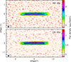 |
Fig. 1. High-resolution images of the continuum emission from the Flying Saucer disk at 230 and 345 GHz. Contour levels are in steps of 4σ (0.16 and 0.13 K, respectively). The images were rotated by 3.1° clockwise to align the disk major axis along the X axis. |
3. Analysis and modeling
3.1. Direct analysis of dust emission
Figure A.1 reveals an apparent spectral index below 2. This is suggestive of a relatively low kinetic temperature, for which the deviations from the Rayleigh Jeans regime are larger at 345 GHz than at 230 GHz. In the uniform slab approximation, we find a Tb(230)/Tb(345) brightness ratio of 1.25 in the 0–140 au range (see Fig. A.2). Although such a ratio can be obtained from blackbody emission at 13 K, with the moderate dust opacities (0.2–0.5) lower temperatures are required because for all reasonable dust properties the opacity is larger at 345 GHz than at 230 GHz (see Appendix B).
3.2. The dust disk shadow onto the CO extended emission
The Flying Saucer lies in front of several molecular clouds that emit in CO at different velocities and with different intensities (Guilloteau et al. 2016), creating a disk shadow clearly seen in the new high-angular-resolution 12CO 2–1 channel maps (Fig. A.3). We used the “shadow” method developed by Guilloteau et al. (2016) (see details in our Appendix D) to repeat their analysis at our much improved angular resolution. A nearly constant temperature of ∼5.5 K is obtained across the disk, except toward the disk center, where it rises up to 10 K in the inner 20 au.
Another way to derive the temperature is to note that when the dust brightness matches that of the background at a specific velocity, v, Jν(Tdust) = Jcloud(v)+Jbg, the leftover signal, Jline(v), vanishes. From the position-velocity map in Fig. B.1, we computed the average spectra from the disk mid-plane between 24 and 180 au, and –24 and –180 au, displayed in Fig. 2 (in blue and red, respectively) with the background CO spectrum from the 30-m (in black). Whenever the computed spectra are 0, the dust (brightness) temperature is directly given by the CO spectrum intensity. Using the parts of the spectra that are not contaminated by CO emission from the disk (low velocities of the red spectrum, and high velocities of the blue one), and after correction for the cosmic background and Rayleigh Jeans deviation, we find dust temperatures of 5.2 K and 5.4 K. These meantemperatures are quite consistent with the median value derived before. From these shadow methods, we thus conservatively estimate that the dust temperature is roughly constant between 20 au and the disk edge, 180 au, with a mean value of 5.5 ± 0.5 K.
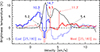 |
Fig. 2. Dust and CO temperature derivation. Numbers indicate the intrinsic temperatures corresponding to the CO cloud brightness temperature at the positions of nulls in the east (blue) and west (red) average mid-plane spectra. The black values are the ones obtained for the dust. |
3.3. Gas temperature determined from the background
There are (four) other zeros in the two disk mid-plane spectra of Fig. 2, at velocities at which CO emission from the disk occurs. In principle, this can provide a measurement of the CO gas temperature. However, this cannot be done in the same way as for dust because of a lack of an external reference (CO without any background). The analysis, whose details and limitations are presented in Appendix B.3, indicates that the absorption of the CO background happens in gas with (mean) temperatures in the range of 10–15 K, since CO is likely to be thermalized.
3.4. Dust temperature from disk model fitting
To obtain an independent estimate of the dust temperature, we fit the continuum emission using a simple inclined disk model, using the ray tracing DiskFit tool (Piétu et al. 2007). We followed the method explained in Guilloteau et al. (2011), using a simple power law distribution for the dust surface density and temperature, radially truncated at an inner and outer radii. The disk is flared, with a Gaussian distribution in density as a function of distance to the mid-plane, and its scale height is a power law of the radius. The dust temperature only depends on the radius.
We simultaneously fit the 230 and 345 GHz data, assuming that the dust opacity is given by κ(ν) = κ0(ν/ν0)β(r) with the exponent following the prescription of Guilloteau et al. (2011), β(r) = β0 + βrlog(r/R0), with κ(230 GHz) = 3.5 cm2 per gram of dust. We derived the H2 surface density assuming a dust to gas ratio of 100. We used a modified Levenberg-Marquardt minimization method, with several starting parameter sets to avoid local minima. Error bars were derived from the covariance matrix. Model parameters, best fit results, and errors are given in Table 1 (see also Appendix D). Most parameters are well constrained, although only an upper limit for the inner radius could be found. Using this best-fit model yields a typical optical depth of 0.1–0.5 across the disk (see Appendix C).
Dust and CO disk modeling results.
With only two observing frequencies, the error bar on the temperature remains significant because of the degeneracy with the opacity law (Boehler et al. 2013). With our adopted opacity, the total disk mass is about 0.009 M⊙.
3.5. Gas temperature from CO disk model fitting
To represent the CO emission, we assume a disk model that has a vertical temperature gradient (Dartois et al. 2003), following the prescription from Dutrey et al. (2017), Foucher (2025) (see Appendix D). The scale height is assumed to be a power law, H(r) = H0(r/R0)−h, and to represent the lack of CO emission in the mid-plane (see Figs. A.3 and B.1) we assume that CO is not present below some depletion scale, zd, i.e., for z < zd = ZdH(r). The CO surface density follows a power law. The disk is truncated at inner and outer radii, Rint and Rout.
The radiative transfer was solved by the DISKFIT code, using the 30-m CO spectrum from Guilloteau et al. (2016), shown in Fig. 2, as a background for ray-tracing as a function of velocities. Parameters were adjusted by a minimization based on a visibility comparison in the uv plane to propagate noise-induced error bars (see Piétu et al. 2007). Results are given in Table 1. The surface density law has little impact on the other results (except for the outer radius, which weakly depends on it) because the core of the CO line remains optically thick in most of the emitting region.
4. Discussion and perspectives
4.1. Mid-plane temperature
Although based on a totally independent high-resolution dataset, the dust temperatures derived through the “disk shadow” are consistent with the ones of Guilloteau et al. (2016), with a dust temperature of 5–6 K. However, DISKFIT yields a higher value, around 9 K, with slightly larger errors due to the coupling between the assumed dust emissivity profiles (function of r and ν) and temperature.
The discrepancy may have several origins. On the one hand, since the single dish spectrum is the same, the absolute temperature scale in the shadow methods remains affected by the same calibration uncertainty. Also, these shadow methods assume no scattering, while self-scattering by dust may reduce the apparent disk brightness (Kataoka et al. 2015); however, the low derived optical depth (∼0.3; see Appendix C) seems to exclude this effect. Finally, the shadow methods also assume that the 30-m spectrum represents uniform emission behind the dust disk. Since the residuals from the best CO model clearly reveal significant structures at scales of 2–10″ (see Fig. A.4), these inhomogeneities may bias the derived dust temperature, especially if combined with spatial structures in the dust disk.
On the other hand, the DISKFIT results for dust are independent of the CO background, but rely on a prescription for the dust emissivity spatial distribution. Given the limited frequency span, this assumption should have little impact on the derived temperature. We thus consider the DISKFIT results to be more reliable, and our observations and analysis indicate low temperatures for the dust, around 9 K, throughout most of the disk. This value agrees remarkably well with the estimated gas temperature in the disk mid-plane. This is to be expected because at the mid-plane densities (given by  from Table 1, 1 to a few 108 cm−3), the dust imposes the gas temperature (Chiang & Goldreich 1997).
Concerning the flat temperature profile of the mid-plane (except within the inner 20 au), we note that non-monotonic temperature profiles may result from the frequency dependence of dust opacity that is controlled by optical properties of grains and grain growth (e.g., Isella et al. 2009, their Fig. 7). These profiles may lead to an apparently flat mid-plane temperature when fit by a simple power law. Such hidden gradients could play a role in explaining the discrepancy found between DISKFIT results and the analysis based on the CO background.
4.2. Gas disk and CO depletion
The CO data indicate a substantial temperature gradient between the mid-plane, with a roughly constant temperature of 10 K, and the upper layers where CO reaches temperatures decreasing from ∼35 K near a radius of 50 au to 15 K at the disk edge. Note, however, that because CO appears depleted in the mid-plane, the mid-plane temperature is essentially a result of the extrapolation of the prescribed shape of the vertical temperature gradient. While there is plenty of evidence of temperature gradients based on the CO isotopologs (e.g., Rosenfeld et al. 2013), measurements of the mid-plane temperature remain rare. Dullemond et al. (2020) measured a mid-plane temperature of 17 K in HD 163296 (based on optically thick CO), but were unable to reach a conclusion about CO depletion in this warmer source.
In previous studies, evidence of CO depletion came from observations of the optically thin emission from isotopologs that allowed one to radially locate the CO “snowline”. The morphology of CO emission in IM Lup (Pinte et al. 2018) is also suggestive of partial CO freeze-out near the mid-plane. Our study of the colder, edge-on disk of the Flying Saucer provides a first quantitative estimate of the thickness of the depleted layer. The best-fit model indicates strong CO depletion below about 0.7 H(r) (at least a factor of 500 to ensure a low optical depth for the 2-1 transition in the mid-plane). Using the derived temperature profile, the temperature at this height varies between 19 K at 100 au to 15 K at 300 au. This is in good agreement with the freeze-out temperature of CO on pure ice (Bisschop et al. 2006; Minissale et al. 2022), although we used a prescribed shape for the depleted layer that did not incorporate any a priori temperature information (see Appendix D). It seems to exclude significant CO to CO2 conversion on grains, which could raise the apparent freeze-out temperature up to 35 K (e.g., Reboussin et al. 2015; Bosman et al. 2018; Ruaud et al. 2022). This latter mechanism may contribute to explaining the higher freeze-out temperatures derived for DM Tau by Qi et al. (2019) and TW Hya by Zhang et al. (2017).
4.3. Dust settling
Boehler et al. (2013) showed that settling may be diagnosed even by fitting a non-settled disk model as was done in Sect. 3.4. In such a case, ignoring settling may affect the disk parameters derived – for example, the surface density profile – or the flaring exponent, −h, which is underestimated. The only strong indicator is the apparent scale height. In our case, the dust scale height (9 au) is not significantly lower than the predicted gas scale height (11 au) if the mid-plane temperature is 10 K (at 100 au). However, the flaring index is −h = 0.9 for dust compared to the expected value of 1.5 for the gas under hydrostatic equilibrium at a constant mid-plane temperature, suggesting larger settling in the less dense outer regions.
Instead of settling, the low flaring index from dust may suggest a self-shadowed disk, leading to low mid-plane temperatures (e.g., Woitke et al. 2016). However, a simple shadowing would result in a steep radial temperature gradient as in GG Tau Dutrey et al. (2014), in contrast to our flat temperature profile. Furthermore, the NIR images from Grosso et al. (2003) indicate a flared morphology consistent with a flaring index of 1.25. Note here that the flaring index derived from CO only reflects the location of the bulk of CO emission, and not necessarily the underlying (H2 and He) gas distribution.
The relatively moderate settling may suggest that the Flying Saucer host star is still relatively young, as settling is less efficient in Class I sources (e.g., Villenave et al. 2023). Unfortunately, the stellar properties are not sufficiently known to constrain the system age.
In summary, our study, based on high-angular-resolution data, clearly shows the presence of an important vertical temperature gradient, the gas and dust mid-plane temperature being of the same order of 10 K, while the molecular layer (at about 1.5–2 hydrostatic scale heights) has a temperature derived from CO DISKFIT modeling of 17–23 K. These data also reveal direct evidence of strong CO depletion in the disk mid-plane, up to 0.7 CO scale heights where the temperature reaches 16–18 K. This is consistent with CO freeze-out on grains, but not with significant conversion of CO to CO2 on grain surfaces.
Acknowledgments
This work was supported by “Programme National de Physique Stellaire” (PNPS) and “Programme National de Physique Chimie du Milieu Interstellaire” (PCMI) from INSU/CNRS. This work was partly supported by the Italian Ministero dell Istruzione, Università e Ricerca through the grant Progetti Premiali 2012 – iALMA (CUP C52I13000140001). This project has received funding from the European Union’s Horizon 2020 research and innovation programme via the European Research Council (ERC) Synergy Grant ECOGAL (grant 855130). Y.W.T. acknowledges support through NSTC grant 111-2112-M-001-064- and 112-2112-M-001-066-. This work was also supported by the NKFIH NKKP grant ADVANCED 149943 and the NKFIH excellence grant TKP2021-NKTA-64. This paper makes use of the following ALMA data: ADS/JAO.ALMA#2013.1.00163.S, ADS/JAO.ALMA#2013.1.00387.S and ADS/JAO.ALMA#2023.1.00907.S. ALMA is a partnership of ESO (representing its member states), NSF (USA) and NINS (Japan), together with NRC (Canada), NSTC and ASIAA (Taiwan), and KASI (Republic of Korea), in cooperation with the Republic of Chile. The Joint ALMA Observatory is operated by ESO, AUI/NRAO and NAOJ.
References
- Andrews, S. M., Huang, J., Pérez, L. M., et al. 2018, ApJ, 869, L41 [NASA ADS] [CrossRef] [Google Scholar]
- Birnstiel, T. 2024, ARA&A, 62, 157 [NASA ADS] [CrossRef] [Google Scholar]
- Bisschop, S. E., Fraser, H. J., Öberg, K. I., van Dishoeck, E. F., & Schlemmer, S. 2006, A&A, 449, 1297 [NASA ADS] [CrossRef] [EDP Sciences] [Google Scholar]
- Boehler, Y., Dutrey, A., Guilloteau, S., & Piétu, V. 2013, MNRAS, 431, 1573 [Google Scholar]
- Bosman, A. D., Walsh, C., & van Dishoeck, E. F. 2018, A&A, 618, A182 [NASA ADS] [CrossRef] [EDP Sciences] [Google Scholar]
- Chiang, E. I., & Goldreich, P. 1997, ApJ, 490, 368 [Google Scholar]
- Dartois, E., Dutrey, A., & Guilloteau, S. 2003, A&A, 399, 773 [CrossRef] [EDP Sciences] [Google Scholar]
- Duchêne, G., Ménard, F., Stapelfeldt, K. R., et al. 2024, AJ, 167, 77 [CrossRef] [Google Scholar]
- Dullemond, C. P., Isella, A., Andrews, S. M., Skobleva, I., & Dzyurkevich, N. 2020, A&A, 633, A137 [EDP Sciences] [Google Scholar]
- Dutrey, A., di Folco, E., Guilloteau, S., et al. 2014, Nature, 514, 600 [NASA ADS] [CrossRef] [Google Scholar]
- Dutrey, A., Guilloteau, S., Piétu, V., et al. 2017, A&A, 607, A130 [CrossRef] [EDP Sciences] [Google Scholar]
- Foucher, C., Dutrey, A., Piétu, V., et al. 2025, A&A, Submitted [Google Scholar]
- Fromang, S., & Nelson, R. P. 2009, A&A, 496, 597 [NASA ADS] [CrossRef] [EDP Sciences] [Google Scholar]
- Gaia Collaboration (Vallenari, A., et al.) 2023, A&A, 674, A1 [NASA ADS] [CrossRef] [EDP Sciences] [Google Scholar]
- Gavino, S., Dutrey, A., Wakelam, V., et al. 2021, A&A, 654, A65 [NASA ADS] [CrossRef] [EDP Sciences] [Google Scholar]
- Grosso, N., Alves, J., Wood, K., et al. 2003, ApJ, 586, 296 [Google Scholar]
- Guidi, G., Isella, A., Testi, L., et al. 2022, A&A, 664, A137 [NASA ADS] [CrossRef] [EDP Sciences] [Google Scholar]
- Guilloteau, S., Dutrey, A., Piétu, V., & Boehler, Y. 2011, A&A, 529, A105 [NASA ADS] [CrossRef] [EDP Sciences] [Google Scholar]
- Guilloteau, S., Piétu, V., Chapillon, E., et al. 2016, A&A, 586, L1 [NASA ADS] [CrossRef] [EDP Sciences] [Google Scholar]
- Isella, A., Carpenter, J. M., & Sargent, A. I. 2009, ApJ, 701, 260 [Google Scholar]
- Kataoka, A., Muto, T., Momose, M., et al. 2015, ApJ, 809, 78 [Google Scholar]
- Minissale, M., Aikawa, Y., Bergin, E., et al. 2022, ACS Earth Space Chem., 6, 597 [NASA ADS] [CrossRef] [Google Scholar]
- Öberg, K. I., Facchini, S., & Anderson, D. E. 2023, ARA&A, 61, 287 [CrossRef] [Google Scholar]
- Pérez, L. M., Carpenter, J. M., Chandler, C. J., et al. 2012, ApJ, 760, L17 [CrossRef] [Google Scholar]
- Piétu, V., Dutrey, A., & Guilloteau, S. 2007, A&A, 467, 163 [Google Scholar]
- Pinte, C., Ménard, F., Duchêne, G., et al. 2018, A&A, 609, A47 [NASA ADS] [CrossRef] [EDP Sciences] [Google Scholar]
- Qi, C., Öberg, K. I., Espaillat, C. C., et al. 2019, ApJ, 882, 160 [Google Scholar]
- Reboussin, L., Wakelam, V., Guilloteau, S., Hersant, F., & Dutrey, A. 2015, A&A, 579, A82 [NASA ADS] [CrossRef] [EDP Sciences] [Google Scholar]
- Rosenfeld, K. A., Andrews, S. M., Hughes, A. M., Wilner, D. J., & Qi, C. 2013, ApJ, 774, 16 [Google Scholar]
- Ruaud, M., Gorti, U., & Hollenbach, D. J. 2022, ApJ, 925, 49 [NASA ADS] [CrossRef] [Google Scholar]
- Simon, M., Guilloteau, S., Beck, T. L., et al. 2019, ApJ, 884, 42 [NASA ADS] [CrossRef] [Google Scholar]
- Tazzari, M., Testi, L., Ercolano, B., et al. 2016, A&A, 588, A53 [NASA ADS] [CrossRef] [EDP Sciences] [Google Scholar]
- Tazzari, M., Clarke, C. J., Testi, L., et al. 2021, MNRAS, 506, 2804 [NASA ADS] [CrossRef] [Google Scholar]
- Ueda, T., Okuzumi, S., Kataoka, A., & Flock, M. 2023, A&A, 675, A176 [NASA ADS] [CrossRef] [EDP Sciences] [Google Scholar]
- Villenave, M., Ménard, F., Dent, W. R. F., et al. 2020, A&A, 642, A164 [EDP Sciences] [Google Scholar]
- Villenave, M., Stapelfeldt, K. R., Duchêne, G., et al. 2022, ApJ, 930, 11 [NASA ADS] [CrossRef] [Google Scholar]
- Villenave, M., Podio, L., Duchêne, G., et al. 2023, ApJ, 946, 70 [NASA ADS] [CrossRef] [Google Scholar]
- Woitke, P., Min, M., Pinte, C., et al. 2016, A&A, 586, A103 [NASA ADS] [CrossRef] [EDP Sciences] [Google Scholar]
- Zhang, K., Bergin, E. A., Blake, G. A., Cleeves, L. I., & Schwarz, K. R. 2017, Nat. Astron., 1, 0130 [NASA ADS] [CrossRef] [Google Scholar]
Appendix A: Data reduction
Data were calibrated using the CASA calibration scripts provided by the ALMA observatory. Calibrated visibilities were then exported into UVFITS data format for imaging and further analysis, using the IMAGER package1. Spectral resampling and conversion to the LSR velocity frame were done withing CASA prior to exportation to UVFITS format.
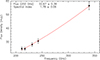 |
Fig. A.1. SED of the Flying Saucer disk in the 200-350 GHz range, with a power law fit superimposed. |
Proper motions: Having different epochs of observations spanning about 10 years, we were able to derive the proper motion of the source by comparing the apparent positions as a function of time, using the continuum data obtained for each dataset. Our proper motion values, μα = −8.4 ± 2.0 and μδ = −27.4 ± 1.5 mas/yr, are consistent with those derived for stars close to the Flying Saucer in ρ Oph (Elias 2-27, YLW 58, and YLW 18) using Gaia (Gaia Collaboration 2023). The distance of the Flying Saucer is unfortunately not known. From Gaia, Elias 2-27 is at 110 pc, while YLW 58 and 18 lie at 135 and 137 pc respectively. Since the Flying Saucer appears in front of molecular clouds, we adopt a distance of 120 pc in this work.
All observations were then registered to Epoch 2016.0 using the derived proper motion, the nominal position of the source being then RA 16:28:13.6979 and declination -24:31:39.491. Self-calibration using the continuum data was performed on the most compact configurations, but not for the most extended ones because the source structure (to first order a bar of apparent size 3 × 0.3″) is heavily resolved and does not leave enough flux on most baselines for this purpose.
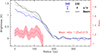 |
Fig. A.2. Radial distribution of the brightness at 235 and 345 GHz along the disk mid-plane (solid black and blue curves). Dashed lines indicate the best-fit model prediction. The brightness ratio is given by the red curve, with the ±1σ confidence interval in pink. |
Flux calibration: Observations at different frequencies and epochs allowed us to derive the apparent spectral index of the continuum emission and check calibration consistency. The two configurations observed in each of Band 6 and Band 7 gave very consistent flux measurements (within < 2 %). However, the older observations from May 2015 (2013.1.00387.S and 2013.2.00163.S) were found to be too bright by about 5 and 7 % respectively, and were rescaled accordingly in flux before being merged with the newer data for imaging and analysis.
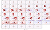 |
Fig. A.3. Channel maps of CO emission. Contour levels are in steps of 4.1 K (≃5σ). Negative signal is in blue and positive in red, with the color scale spanning -23 to 23 K. Panels are labeled by the velocity, in the range -0.95 to 8.42 km s−1. |
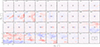 |
Fig. A.4. 12″ field channel maps of the residual emission after model fitting. The color scale spans -23 to 23 K, as in Fig. A.3, but data values in the residual only span the -9 to 9 K range. The box in the bottom-right panel shows the area displayed in Fig. A.3. Note the slightly different velocities compared to Fig. A.3 |
Spectral and continuum imaging: Once the astrometric and flux calibration issues were solved, data from different configurations were combined together. All data was then imaged using a common grid, with a pixel size of 0.025″. Various choices of robust weighting parameters were used in order to offer an adequate compromise between angular resolution, sensitivity and dirty beam shape (to minimize in particular the plateau of near sidelobes that occurs when combining two ALMA array configurations). A field of view of 25.6″ was used for CO to best handle the extended background clouds (although the selected field of view had minor impact on the reconstructed image of the disk itself). The CO synthesized beam is 0.217 × 0.144″ at PA 104°, and the noise level is ∼0.1 K at 0.23 km s−1 spectral resolution.
The continuum images were produced after filtering the spectral line emission using the UV_FILTER command of IMAGER. Bandwidth synthesis was used to obtain the images. The resolution is 0.172 × 0.113″ at PA 100° at 230 GHz, and 0.166 × 0.121″ at PA 90° at 345 GHz. We tested several deconvolution methods, all giving consistent results within the expected noise level for the spectral line observations. The continuum data is however dynamic range limited, with actual noise level 1.5 to 2 times larger than the thermal noise, and dynamic range about 60 at high resolution. All spectral and continuum images were finally rotated by 3.1° clockwise to align the disk major axis along the X axis. Figure A.3 presents the CO channel maps.
Appendix B: Temperature derivation
B.1. Direct analysis of dust emission
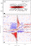 |
Fig. B.1. (a): Integrated CO line flux. Contour spacing is 10 mJy/beam.km/s (7 K.km/s), overlaid on the continuum image (peak brightness is 2 K). (b): Position-velocity diagram across the disk plane. Contour spacing is 2 K, about 2.4 σ. The black curve is the Keplerian velocity for a 0.6 M⊙ star. Negative signal is in blue, positive in red. |
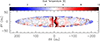 |
Fig. B.2. Mean dust temperature distribution across the disk. Contour steps are 1 K. |
In a uniform slab, the brightness Tb is given by
 (B.1)
(B.1)
where Jν is the radiation temperature, i.e., the Planck function multiplied by c2/2kν2:
 (B.2)
(B.2)
Td the dust temperature, Tbg = 2.7 K the cosmic background temperature, τ the optical depth, and f a beam filling factor < 1. The brightness ratio S23 = Tb(235 GHz)/Tb(345 GHz) can be used to obtain an estimate to Td. Given the similar geometrical thickness and spatial resolution at both frequencies (see Fig. C.1), a common beam filling factor can be used. The uniform slab approximation is reasonable, since S23 is approximately constant at 1.25 between 20 and 120 au (Fig. A.2). In the optically thick limit, or when opacities are equal at both frequencies, this S23 value corresponds to Td = 13 K. However, since for all reasonable dust properties the opacity is larger at 345 GHz than at 230 GHz (their ratio being 1.3 using β from Table 1), this value is an upper limit: a partially optically thin medium would need to be colder.
B.2. The shadow method for dust
As discussed by Guilloteau et al. (2016), the Flying Saucer lies in front of several molecular clouds, which emits in CO at different velocities and with different intensities. The dust disk appears in shadow against this bright, frequency variable background, providing a (so far unique) opportunity to measure the dust temperature in a totally independent way compared to usual methods. The disk shadow can be clearly seen in the high angular resolution 12CO 2-1 channel map shown in Fig. A.3.
The shadow method derives from the basic radiative transfer equation (Eq. B.1) that gives the flux (expressed in brightness), Jm, emerging from a medium of temperature, Tm, as a function of velocity, v:
 (B.3)
(B.3)
Here Jback is the brightness temperature of any spatially extended background, that is removed by the On-Off observing technique with single-dish, or filtered out by interferometers.
Far from the cloud velocities, Jback = Jbg = Jν(Tbg) = 0.19 K at 230 GHz is due to the cosmological background. At velocity v, the dust disk is in front of an extended CO cloud whose apparent brightness, as measured by the IRAM 30-m telescope, is thus
 (B.4)
(B.4)
so that of the dust disk brightness temperature at velocity v becomes
 (B.5)
(B.5)
We call Jdisk the disk continuum brightness temperature away from the cloud velocities. Subtracting the Jdisk and Jline yields the optical depth and beam filling factor product,
 (B.6)
(B.6)
that we use to eliminate from Eq. B.5, and after some re-arrangement we obtain
 (B.7)
(B.7)
A position-velocity map showing Jline(v) across the disk mid-plane is displayed in Fig. B.1. The method can be applied to any line of sight to recover the dust temperature across the disk. The cloud emission being velocity dependent provides several independent estimates for each direction, and we take the median value to obtain the dust temperature map displayed in Fig. B.2. Compared to the Guilloteau et al. (2016) data, the current data improve the spatial resolution by a factor of 2 along the radius and 3 in the vertical direction. A nearly constant temperature of ∼5.5 K is obtained across the disk, except toward the disk center where it rises up to 10 K in the inner 20 au.
Another derivation is possible when Jline(v) = 0 in Eq. B.5, but this only occurs at two velocities, (2.7 and 7.3 km s−1; Fig. 2) providing less redundancy in the determination of Tdust.
B.3. The shadow method for gas
Gas around the disk mid-plane also appears in absorption against the CO clouds. However, contrary to dust, there is no reference emission flux (Jdisk) that we can use to eliminate the f(1 − exp(−τ)) factor. So we are left with the methods relying only on the zero values of Eq. B.5 found at some velocities in Fig. 2, where neither f nor τ matters. This method has a number of limitations, however.
First, the spectrum in Fig. 2 being an average over the disk radii, at velocity offsets dV larger than 1.7 km s−1 from the systemic velocity (3.70 km s−1) emission only comes from regions smaller than r(dV) = (G M*)/dV2 = 100 (2.3/dV)2 au due to the Keplerian rotation (see Fig. B.1). Therefore, the mean CO brightness temperature is only valid up to this radius. Fortunately, all zeros are within the [2.0,5.4] km s−1 velocity range and do not need to be corrected. Strictly speaking, a similar correction is also needed for emission near the systemic velocity, since it only extends up to 80-100 au because of the velocity projection, but this does not affect the position (in velocity) of the zero.
Second, the disk may (or may not) be optically thick in CO, hiding (part of) the dust emission. However, this is a small effect on the apparent brightness (only 0.2 K) that we can neglect.
Third, Eq. B.5 is for a homogeneous medium. In practice, we only measure the average brightness temperature, and its value can be interpreted as being due to either cold gas filling the beam, or warmer gas with a smaller filling factor. Assuming f = 1, we get temperatures ranging from 9.5 K to 14.7 K. The temperature of 9.5 K appearing in Fig. 2 at 3.7 km s−1 does not account for the apparent disk extent (caused by the velocity gradient) at this velocity. Using a more appropriate beam filling factor of 0.5 for this case raises the temperature to 14.2 K.
Appendix C: Dust optical depth
Direct determination: We can estimate the dust optical depth by comparing the apparent brightness of the continuum to the temperature derived from the shadow, but this requires an estimate of the beam filling factor f. Since the disk is well resolved in radius, f is controlled by the thickness. The intrinsic thickness is derived (to first order) by deconvolving the apparent thickness from the effective resolution, here the beam minor axis, as the beams are essentially elongated parallel to the radius. Apparent sizes were derived by Gaussian fit to the observed (vertical) profile. Apparent and corrected sizes are displayed as a function of radius in Fig. C.1. The mean filling factor is 0.83. It should be noted that this correction is an underestimate of the required one, because the images are dynamic range limited due to significant phase noise remaining on the long baselines. This results in a seeing effect that should be combined in quadrature with the beam size. This may bring down the beam filling factor to 0.7, for which the peak brightness still only reaches 2.2 K from Fig. A.2. When compared to the estimated dust temperature, 9 K, this indicates dust opacities of order 0.25.
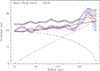 |
Fig. C.1. Apparent (black) and intrinsic (red) thickness of the continuum emission at 230 GHz as a function of radius. In blue, we show the intrinsic thickness at 345 GHz. The dash-dotted line indicates the width due to the best-fit scale height, the dashed line the expected width due to the disk inclination of ∼86°, and the solid line the resulting total width. |
From the model: While the DISKFIT tool can produce optical depth maps for the best fit model parameters, a simple analytical verification is possible because, for dust, the best fit model is essentially one of an isothermal, uniform surface density disk. In this vertically isothermal dust disk, the mid-plane density is given by
 (C.1)
(C.1)
since −p + h ≈ −1 (see Table 1), R0 = 100 au being the reference radius at which Σg is given.
Assuming edge-on geometry, at an impact parameter R, the line of sight optical depth in the midplane is approximately given by
 (C.2)
(C.2)
(provided R remains reasonably small compared to Rout, which allows us to ignore the incidence angle at each radius, an approximation that is valid up to about 120 au), i.e.,
 (C.3)
(C.3)
 (C.4)
(C.4)
which gives τ(R, 235 GHz)≈0.2log(Rout/R) using numbers from Table 1, yielding τ(70 au, 235 GHz) = 0.2 in the mid-plane. The disk becomes optically thick only for radii smaller than 2 au, consistent with an inner radius upper limit found in the minimization process. In this edge-on assumption, the opacity decreases with the dust scale height. The small tilt from edge-on view will slightly smear out the opacity distribution.
Appendix D: Disk model
In our disk model, the density distribution is assumed to be a Gaussian as a function of height z above the mid-plane, n(r, z) = n0exp(−(z/H(r))2), with a scale height being a power law, H(r) = H0(r/R0)−h, and the gas temperature distribution is
 (D.1)
(D.1)
for z < zq, and Tatm(r) above, with the “atmosphere” temperature given by
 (D.2)
(D.2)
and the mid-plane temperature by
 (D.3)
(D.3)
Here zq indicates the start of the (isothermal) atmosphere, δ the gradient steepness. For δ ≃ 1 the steepest gradient is in the transition zone between mid-plane and atmosphere at zqH(r)/2. We do not impose the scale height to be related to the mid-plane temperature. Instead, it is determined to represent the distribution of the CO molecules that best fit the observed data, with the further assumption that no CO is present below a depletion height zd = ZdH(r), where Zd is another fit parameter in the model.
To reproduce the velocity pattern, we also account for the geometric and kinematics parameters: orientation (PA = 3.1 ± 0.2°), inclination (i = 86.3 ± 0.2°), systemic velocity (VLSR = 3.71 ± 0.01 km s−1), stellar mass (M* = 0.59 ± 0.01 M⊙), and local line width (δV = 0.20 ± 0.01 km s−1, assumed constant across the disk). These parameters are not significantly coupled to any of the others. With power laws for surface density and scale heights, our model cannot represent the disk edge shape, and only yields results relevant to the 50 au to 250 au radius range.
Significant coupling exists between Tmid, Zd, H0 and δ. To alleviate this problem, we performed fits fixing one parameter and solving for the others. We also explored an alternate functional shape, that is equivalent to Eq. D.1 only if δ = 1, namely
 (D.4)
(D.4)
All explored cases yielded low Tmid, and the temperature at z = zd was always around 17 K.
All Tables
All Figures
|
Fig. 1. High-resolution images of the continuum emission from the Flying Saucer disk at 230 and 345 GHz. Contour levels are in steps of 4σ (0.16 and 0.13 K, respectively). The images were rotated by 3.1° clockwise to align the disk major axis along the X axis. |
| In the text | |
|
Fig. 2. Dust and CO temperature derivation. Numbers indicate the intrinsic temperatures corresponding to the CO cloud brightness temperature at the positions of nulls in the east (blue) and west (red) average mid-plane spectra. The black values are the ones obtained for the dust. |
| In the text | |
|
Fig. A.1. SED of the Flying Saucer disk in the 200-350 GHz range, with a power law fit superimposed. |
| In the text | |
|
Fig. A.2. Radial distribution of the brightness at 235 and 345 GHz along the disk mid-plane (solid black and blue curves). Dashed lines indicate the best-fit model prediction. The brightness ratio is given by the red curve, with the ±1σ confidence interval in pink. |
| In the text | |
|
Fig. A.3. Channel maps of CO emission. Contour levels are in steps of 4.1 K (≃5σ). Negative signal is in blue and positive in red, with the color scale spanning -23 to 23 K. Panels are labeled by the velocity, in the range -0.95 to 8.42 km s−1. |
| In the text | |
|
Fig. A.4. 12″ field channel maps of the residual emission after model fitting. The color scale spans -23 to 23 K, as in Fig. A.3, but data values in the residual only span the -9 to 9 K range. The box in the bottom-right panel shows the area displayed in Fig. A.3. Note the slightly different velocities compared to Fig. A.3 |
| In the text | |
|
Fig. B.1. (a): Integrated CO line flux. Contour spacing is 10 mJy/beam.km/s (7 K.km/s), overlaid on the continuum image (peak brightness is 2 K). (b): Position-velocity diagram across the disk plane. Contour spacing is 2 K, about 2.4 σ. The black curve is the Keplerian velocity for a 0.6 M⊙ star. Negative signal is in blue, positive in red. |
| In the text | |
|
Fig. B.2. Mean dust temperature distribution across the disk. Contour steps are 1 K. |
| In the text | |
|
Fig. C.1. Apparent (black) and intrinsic (red) thickness of the continuum emission at 230 GHz as a function of radius. In blue, we show the intrinsic thickness at 345 GHz. The dash-dotted line indicates the width due to the best-fit scale height, the dashed line the expected width due to the disk inclination of ∼86°, and the solid line the resulting total width. |
| In the text | |
Current usage metrics show cumulative count of Article Views (full-text article views including HTML views, PDF and ePub downloads, according to the available data) and Abstracts Views on Vision4Press platform.
Data correspond to usage on the plateform after 2015. The current usage metrics is available 48-96 hours after online publication and is updated daily on week days.
Initial download of the metrics may take a while.