© The Authors 2025

1. Introduction

Relativistic jets produced by active galactic nuclei (AGNs) represent ideal laboratories for addressing several topics related to black hole physics, particle acceleration, and high-energy (and possible multi-messenger) emission (e.g., Blandford et al. 2019). Jets are best studied in blazars, where a favorable geometrical alignment leads to the relativistic amplification of the nonthermal radiation produced in the jet by relativistic particles (Romero et al. 2017). Blazars are characterized by a double-humped spectral energy distribution (SED), with the first hump peaking in the IR-soft-X-ray band and the high-energy hump peaking at gamma-ray energies (e.g., Fossati et al. 1998). There is general consensus that the first hump is produced by leptons (electrons or pairs) through synchrotron emission. According to the standard framework (e.g., Sikora et al. 1994; Ghisellini et al. 1998), the same particles up-scatter soft radiation, forming the high-energy hump through the inverse Compton (IC) mechanism. A competing scenario assumes instead that the high-energy hump is produced by relativistic hadrons, either through direct proton-synchrotron emission or through synchrotron emission by the by-products of hadronic reactions (see Sol & Zech 2022 for a review). The hadronic scenario is supported by the potential association of some blazars with high-energy neutrinos (e.g., Böttcher 2019).

The Imaging X-ray Polarimetry Explorer (IXPE) satellite (Weisskopf et al. 2022) enables multifrequency polarimetric observations of blazars that, in principle, can offer unique clues as to the physical processes acting in these sources. In particular, it has been anticipated that the polarimetric properties of the X-ray emission of blazars can be used to determine the emission mechanism responsible for the high-energy hump (e.g., Zhang 2017; Peirson et al. 2022). This can be done in low- and intermediate-synchrotron-peaked (LSP and ISP) blazars (Abdo et al. 2010), where the X-rays trace the rising portion of the high-energy hump. The general idea is that in single-zone models with nearly uniform fields, hadronic processes lead to a high polarization of the radiation in this band because X-rays are produced through synchrotron emission, either by high-energy protons or by the by-products of hadronic reactions (Zhang & Böttcher 2013). On the other hand, leptonic models lead to a lower polarization because the X-rays are produced through IC emission. The IC radiation would be unpolarized when the seed photons are thermal and isotropic, such as photons produced in the central regions of the AGN (Bonometto & Saggion 1973), and would have a low degree of polarization (≲50% of the degree of polarization of the seed photons) when it is produced through the synchrotron self-Compton (SSC) mechanism (Poutanen 1994; Krawczynski 2012). The comparison between the polarization in the optical band (produced through synchrotron radiation by high-energy electrons) and in the X-ray band would therefore be a powerful diagnostic of the emission mechanism at work.

Agudo et al. (2025) report multifrequency polarimetric observations of BL Lac, a well-studied LSP/ISP-type blazar. The optical emission, which belongs to the soft tail of the low-energy SED component, showed an exceptionally high (and variable) degree of polarization (average of 25%, reaching 45%). IXPE obtained a quite constraining upper limit of ∼7% for the degree of polarization in the X-ray band, which tracks the rising part of the high-energy SED peak. Agudo et al. (2025) conclude that these measurements strongly support the leptonic scenario, in which the X-rays are produced through IC scattering by the same electrons that produce the radio-to-optical component through synchrotron emission. This result strengthens previous similar results by IXPE for BL Lac (Middei et al. 2023; Peirson et al. 2023) and other sources of the LSP class (Marshall et al. 2024). A follow-up modeling of the source was carried out by Liodakis et al. (2025), who conclude that, regardless of the jet composition and the assumed emission model, IC scattering from relativistic electrons dominates the X-ray regime. Their study considered four scenarios for the high-energy spectral component: a pure SSC model, a SSC + external Compton leptonic model, a hybrid model involving SSC and hadronic processes, and a purely hadronic model.

Given the relevance of the topic, it is important to more thoroughly investigate the hadronic scenarios, which are disfavored by the studies of Agudo et al. (2025) and Liodakis et al. (2025). Here we discuss a scenario in which the high-energy component is produced by high-energy hadrons (protons in the following) through synchrotron emission (e.g., Aharonian 2000; Zech et al. 2017; Liodakis & Petropoulou 2020). We determined the jet magnetic fields from a magnetohydrodynamic model of magnetically dominated stationary axisymmetric outflows (e.g., Vlahakis 2004; Lyubarsky 2009). The degree of polarization of synchrotron radiation depends on the shape of the jet, the size of the emission region, and the slope of the energy distribution of the emitting particles (Bolis et al. 2024a). We emphasize that the dependence on the slope of the particle distribution is stronger than in the textbook case of a uniform field. The low degree of polarization in the X-ray band is naturally produced by the joint effect of (i) the hard slope of the underlying proton energy distribution and (ii) the larger region encompassed by the slow-cooling protons with respect to the fast-cooling electrons responsible for the optical emission.

The paper is organized as follows. In Sect. 2 we present the model and the calculation of the polarization, and in Sect. 3 we discuss the results. Throughout the paper, the following cosmological parameters are assumed: H₀ = 70 km s⁻¹ Mpc⁻¹, Ω_M = 0.3, and Ω_Λ = 0.7.

2. The model

2.1. Model set-up

Our aim is to show that multifrequency polarization observations of BL Lac can be explained by a model where the X-rays are produced through the proton-synchrotron mechanism. Our model follows the work of Bolis et al. (2024a), which discusses the polarization of synchrotron radiation from magnetically dominated jets. The main result of that work is the following. The degree of polarization has a strong dependence on the slope of the energy distribution of the emitting particles (see also Bolis et al. 2024b). This feature can be important to explain the strong chromaticity of the observed degree of polarization in high-synchrotron peaked blazars. Here, we extend the model of Bolis et al. (2024a), including the emission from a population of high-energy protons that fill a region of non-negligible thickness.

Our scenario is sketched in Fig. 1. The transverse radius of the jet, R₀, and the distance from the central black hole, z₀, are related by R₀ ∝ z₀^q. The jet carries a helical magnetic field (see below for more details). At some distance z₀ ∼ 10¹⁷ cm from the black hole, particles (electrons and protons) are accelerated to relativistic energies by an unspecified acceleration mechanism and subsequently cool, emitting synchrotron radiation. We assumed that the first component of the SED is produced by the electrons and the second component by synchrotron radiation from protons. To produce photons at the peak of the high-energy hump, which is located around E ∼ 100 MeV, protons have energies on the order of (Aharonian 2000)¹

$$\begin{array}{c}\hfill {\gamma }_{\mathrm{p},\max }^{\prime }\simeq {\left(\frac{4\pi m_{p}cE}{3eh{B}^{\prime }\delta }\right)}^{1/2}\simeq 3\times {10}^8{B}_1^{\prime -1/2}{\delta }_1^{-1/2},\end{array}$$(1)

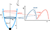Fig. 1. Sketch of the scenario discussed in the text. The jet has a parabolic shape and carries a helical magnetic field. Particles are accelerated at some distance (z0) from the black hole. Electrons, which have a very short cooling time, produce the optical emission in a thin shell close to the acceleration zone. Protons, instead, are in the slow-cooling regime and are advected by the flow up to a distance Δz ∼ z0 (determined by the adiabatic energy losses). Protons produce the high-energy component of the SED, including the X-rays.

where e is the electron charge, h is the Planck constant, c the speed of light, and m_p the protons mass. We use the standard notation B′ = 10 B′₁ G and δ = 10 δ₁, where B′ is the magnetic field and δ is the Doppler factor. In the following, we assume fiducial values B′ = 10 G and δ = 10. We also assume a viewing angle θ_obs = 0.1 rad, which implies a bulk Lorentz factor Γ = 10.

The magnetic field is sufficient to confine the protons up to the energy required to produce the high-energy peak, which is $E{\prime }_{\mathrm{p},\max }=\gamma {\prime }_{\mathrm{p},\max }{m}_{\mathrm{p}}{c}^2=3\times {10}^{17}\mathrm{eV}$ (assuming a jet transverse radius R ∼ 10¹⁶ cm, the classical Hillas limit (Hillas 1984) gives $E_{\mathrm{p}}^{\prime }\lesssim e{B}^{\prime }R\sim {10}^{19}\mathrm{eV}$). Moreover, one can easily check that the strong magnetic field suppresses the SSC emission, which provides a negligible contribution to the observed emission (see Appendix A). Finally, photomeson and Bethe-Heitler losses of protons are also negligible with respect to synchrotron².

For the adopted strength of the magnetic field, the protons that produce the X-ray emission (at 5 keV, the center of the IXPE band) have a Lorentz factor $\gamma {\prime }_{\mathrm{p}}\simeq 4\times {10}^6$ (given by Eq. (1) with E = 5 keV), while the electrons responsible for the optical emission have a Lorentz factor $\gamma {\prime }_{\mathrm{e}}\simeq {10}^3$. The cooling length of the emitting electrons and protons is an important quantity in our model. Electrons are characterized by very efficient radiative losses and, therefore, by a very short cooling length (l_e, cool):

$$\begin{array}{c}\hfill l_{\mathrm{e},\mathrm{cool}}=c\frac{{\gamma }_{\mathrm{e}}^{\prime }}{\dot{{\gamma }_{\mathrm{e}}^{\prime }}}\mathrm{\Gamma }=\frac{6\pi m_{\mathrm{e}}{c}^2}{{\sigma }_{\mathrm{T}}{B^{\prime }}^2{\gamma }_{\mathrm{e}}^{\prime }}\mathrm{\Gamma }\simeq 3\times {10}^{15}\mathrm{cm}\ll z_0,\end{array}$$(2)

where σ_T is the Thomson cross section and m_e the electron mass. On the other hand, protons are in the slow-cooling regime and, therefore, their energy losses (even at the highest energies) are dominated by adiabatic expansion. The typical length scale of adiabatic cooling, l_p, cool = Δz ≃ 3z₀/2q, is on the order of a few z₀ (see Appendix B). Therefore, while electrons emit optical radiation in a very thin slice, coincident with the acceleration region, the X-ray emission is produced by protons, advected by the plasma, that fill a much larger volume (see Fig. 1). As we show below, this is important to further reduce the polarization of the X-ray emission.

For the jet parameters assumed above, the energy flux associated with the protons is on the order of P_p = 3 × 10⁴⁵ erg s⁻¹ (see Appendix C). The magnetic field carries an energy flux about ten times larger, P_B = 3 × 10⁴⁶ erg s⁻¹. The jet is thus dominated by the Poynting flux, consistent with our assumptions. The total jet power is close but below the Eddington luminosity of the central supermassive black hole, which is L_Edd = 6.5 × 10⁴⁶ erg s⁻¹ for a black hole mass M_BH ≃ 5 × 10⁸ M_⊙ (Capetti et al. 2010).

2.2. Polarization

In the following, we sketch the polarization degree calculation, which is presented in detail by Bolis et al. (2024a,b). We determined the magnetic fields of the jet from a magnetohydrodynamic model of magnetically dominated stationary axisymmetric outflows confined by an external medium (Lyubarsky 2009). We assumed that the pressure profile of the external medium decreases as a power law, 𝒫_ext ∝ z₀^−κ, where z₀ is the distance from the black hole. In this case, the transverse radius of the jet, R₀, scales as R₀ ∝ z₀^q. The parameter q depends on the external pressure profile. The jet has a parabolic shape for a wind-like medium (κ = 2), with 1/2 < q < 1.

Adopting cylindrical coordinates, the electromagnetic fields in the observer frame can be written as

$$\begin{array}{cc}\hfill \mathbf{E}& =E_R\widehat{\mathbf{R}}+E_z\widehat{\mathbf{z}}\hfill \end{array}$$(3)

$$\begin{array}{cc}\hfill \mathbf{B}& =B_R\widehat{\mathbf{R}}+B_{\varphi }\widehat{\mathit{\varphi }}+B_z\widehat{\mathbf{z}},\hfill \end{array}$$(4)

where

$$\begin{array}{cccc}\hfill E_R& =\mathrm{\Omega }R{B}_{\mathrm{p}}cos\mathrm{\Theta },\hfill & \hfill E_z& =-\mathrm{\Omega }R{B}_{\mathrm{p}}sin\mathrm{\Theta }\hfill \end{array}$$(5)

$$\begin{array}{cccc}\hfill B_R& =B_{\mathrm{p}}sin\mathrm{\Theta },\hfill & \hfill B_z& =B_{\mathrm{p}}cos\mathrm{\Theta }.\hfill \end{array}$$(6)

In this section the speed of light was set to c = 1. The angular velocity, Ω, and the poloidal magnetic field, B_p, are independent of R. The transverse radius of the jet is given by ΩR₀ = 3^1/4(Ωz₀)^q. The jet opening angle, Θ, and the toroidal magnetic field are given by (Lyubarsky 2009; Bolis et al. 2024a)

$$\begin{array}{cc}\hfill \mathrm{\Theta }& =q\frac{R}{R_0}\frac{3^{1/4q}}{{\left(\mathrm{\Omega }{R}_0\right)}^{(1-q)/q}}\hfill \end{array}$$(7)

$$\begin{array}{cc}\hfill \frac{B_{\varphi }^2-E^2}{B_{\mathrm{p}}^2}& =3^{-1+1/2q}q(1-q)\frac{{\left(\mathrm{\Omega }R\right)}^4}{{\left(\mathrm{\Omega }{R}_0\right)}^{2/q}}.\hfill \end{array}$$(8)

We assumed that the bulk velocity of the fluid, v, coincides with the drift velocity, as appropriate for Poynting-dominated outflows: v = E × B/B². The corresponding bulk Lorentz factor is Γ = (1 − v²)^−1/2 = (1 − E²/B²)^−1/2. The value of ΩR₀ was determined from the condition Γ(R₀) = 10, which corresponds to the typical Lorentz factor of AGN jets.

We assumed that the distribution of the emitting particles (electrons and protons) in the fluid proper frame is isotropic in momentum. We also assumed that the distribution is a power law in energy, $N_{\mathrm{e},\mathrm{p}}\prime ({\gamma }_{\mathrm{e},\mathrm{p}}\prime )=K_{\mathrm{e},\mathrm{p}}{\gamma }_{\mathrm{e},\mathrm{p}}^{\prime -p}$, where K_e, p(R, z) is the proper particle number density and ${\gamma }_{\mathrm{e},\mathrm{p}}\prime$ is the particle Lorentz factor.

The linear degree of polarization, Π, and the electric vector position angle, Ψ, of the synchrotron radiation from the entire emission region (assumed to be unresolved), are respectively given by³

$$\begin{array}{cc}\hfill \mathrm{\Pi }& =\frac{\sqrt{Q^2+U^2}}{I}\hfill \end{array}$$(9)

$$\begin{array}{cc}\hfill tan2\mathrm{\Psi }& =\frac{U}{Q},\mathrm{where}0<\mathrm{\Psi }<\pi .\hfill \end{array}$$(10)

The Stokes parameters I, Q, and U are calculated in Appendix D. We had to define the particle number density of electrons and protons, K_e, p. As in Bolis et al. (2024a), we considered two scenarios: K_e, p = K₀, which corresponds to a constant number density in the proper frame of the fluid, and K_e, p ∝ B^′2 = B²/Γ², which corresponds to constant magnetization.

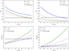Fig. 2. X-ray polarization degree, ΠX (top panels) and chromaticity, ΠO/ΠX (bottom panels) as a function of the width of the proton emission region, Δz. In the left panels, the proper number density is assumed to be constant, whereas in the right panels, the magnetization is assumed to be constant. The X-ray polarization degree is ΠX = Πpp = 2.3, and the optical polarization degree is ΠO = Πpe = 4.6. The viewing angle is assumed to be θobs = 0.1 rad.

2.3. Results

The optical emission is due to synchrotron radiation from nonthermal electrons, whereas we assumed that the X-ray emission is produced through the proton-synchrotron mechanism. As discussed above, in order to calculate the polarization of synchrotron radiation, we assumed that the emitting electrons are confined within an infinitely thin shell (i.e., Δz → 0), whereas the protons propagate to large distances, filling a volume with 0 < Δz < 4z₀. We assumed that the electrons emitting in the optical band have a slope p_e = 4.6 and that the protons emitting in the X-ray band have p_p = 2.3 (Agudo et al. 2025).

Our results are summarized in Table 1 and Fig. 2. In the top panels of Fig. 3 we show the observed degree of polarization in the X-ray band as a function of the length of the emission region in units of the distance from the black hole, Δz/z₀. We consider different jet shapes, described by the parameter q. In the left panel, we assume that the density in the proper frame is constant, whereas in the right panel we assume that the magnetization is constant. In the bottom panels, we show the ratio between the degree of polarization in optical and X-rays. The observed degree of polarization (average Π_O ∼ 25 − 30% and Π_X < 7%) can be reproduced in both cases (constant number density or constant magnetization) for q = 0.6 − 0.7 and Δz ≳ 3. In general, the case of constant number density leads to higher values of Π_O, and the case of constant magnetization leads to smaller Π_X. The electric vector position angle, which is the same for X-ray and optical emission (consistent with the observations), is aligned with the jet axis.

In Appendix E we show the degree of polarization in the X-rays (for a fixed Δz/z₀ = 3) and in the optical band as a function of the viewing angle θ_obs. Generally, the degree of polarization is proportional to θ_obs² (Bolis et al. 2024b). We emphasize that, in the case of constant magnetization, a larger Π_O can be obtained for θ_obs ≳ 0.1 rad, while Π_X is safely below the IXPE limit.

3. Discussion

Multifrequency polarimetric observations of BL Lac show different degrees of polarization in the optical band and in the X-rays, which is interpreted as evidence that the origin of the X-rays is leptonic (Agudo et al. 2025; Liodakis et al. 2025). We have shown that these observations can also be explained by a hadronic model, where optical radiation is produced through synchrotron emission by relativistic electrons (or, more generally, leptons) and X-rays are produced through the proton-synchrotron mechanism.

The significant difference between the polarization of the synchrotron radiation from the two species is due to the following effects: (i) the different slopes of the underlying particle energy distributions (with slopes p_e = 4.6 and p_p = 2.3 for electrons and protons, respectively), and (ii) the larger emission volume of the protons, which have a longer cooling length. In our model we assumed a globally ordered magnetic field. The introduction of turbulence at intermediate spatial scales would likely further reduce the degree of polarization in the X-ray band (Bandiera & Petruk 2016, 2024).

In our scenario, synchrotron emission is the main radiative channel for protons. Photomeson production, considering only the photons internally produced in the jet, provides a negligible contribution⁴. However, as commonly found in hadronic scenarios, the radiative cooling times are very long and the proton energy losses are dictated by adiabatic expansion, resulting in a cooling length comparable to the distance of the emitting region from the central black hole. Despite the low radiative efficiency, a recognized problem for hadronic models (e.g., Zdziarski & Bottcher 2015), in our model the jet energy flux required to power the observed emission is below the Eddington luminosity of the associated black hole.

Liodakis et al. (2025) explored a hybrid leptonic-hadronic (SSC+hadronic) scenario and a purely hadronic model to interpret the observed variability and polarization signatures of BL Lac. They conclude that their hadronic scenarios cannot reproduce observations due to the long proton cooling time (only radiative losses were considered, and therefore the predicted variability timescale at X-ray/gamma-ray energies is on the order of several years) and the degree of polarization being significantly higher than the IXPE upper limit. Both problems are solved in our model, where the cooling time is dictated by adiabatic losses (which are much more effective than radiative losses) and the polarization is intrinsically low.

In this work we considered a stationary model suitable for reproducing the average polarimetric quantities reported by Agudo et al. (2025). One striking result of the monitoring is the large variability observed in the optical band for both the flux and the degree of polarization (accompanied by moderate activity in the X-ray band). In particular, the degree of polarization displayed a symmetric “flare” of about 10 days with variations of 10–45%. In the framework of our model, this behavior could be reproduced by a small emission region (possibly caused by magnetic reconnection) moving on a helical path with the drift velocity (e.g., Di Gesu et al. 2023; Pacciani et al. 2025). This scheme naturally predicts an intensity flare accompanied by a large increase in the degree of polarization (approaching values corresponding to a uniform field) when the beamed emission of the moving feature is directed toward the observer. The detailed model will be reported elsewhere (Bolis et al. in prep.).

In this work we focused on the optical and X-ray bands. As is usual for blazar models, the radio data span a spectral region where synchrotron self-absorption is expected to be important. In this particular case, the very hard spectrum reported in Table 4 of Agudo et al. (2025) implies that the emission is already partly self-absorbed at frequencies around 10¹² Hz. The radio emission comes from a region of the jet that is located farther downstream with respect to the region where the optical and X-ray emission is produced. Therefore, our scheme does not allow us to estimate the polarimetric properties of radio emission.

In view of future missions with polarimetric capabilities in the MeV (and possibly GeV) bands, for example the Compton Spectrometer and Imager (COSI; Tomsick & COSI Collaboration 2022), it is useful to look at the expected polarimetric properties in these bands. The high-energy spectrum of BL Lac (and of LSP blazars in general) approximately maintains the same slope up to the peak around 100 MeV. Since the cooling length of protons is determined by the adiabatic losses, which are independent of energy, we expect a similar low degree of polarization in the MeV and X-ray bands. On the other hand, after the high-energy SED peak (E > 100 MeV), the softening of the spectrum determines the increase in the degree of polarization, which could reach 15–20% in the scenario with constant density.

Acknowledgments

We thank the referee for useful comments. We acknowledge financial support from an INAF Theory Grant 2022 (PI F. Tavecchio) and from a Rita Levi Montalcini fellowship (PI E. Sobacchi). This work has been funded by the European Union-Next Generation EU, PRIN 2022 RFF M4C21.1 (2022C9TNNX). This work has been funded by ASI under contract 2024-11-HH.0.

References

Appendix A: Limit on SSC emission

For a source with observed synchrotron luminosity L_s (for BL Lac, one has L_s ∼ 10⁴⁵ erg s⁻¹), the luminosity of the SSC emission can be estimated as

$$\begin{array}{c}\hfill L_{\mathrm{SSC}}=\frac{U_{\mathrm{s}}^{\prime }}{U_{\mathrm{B}}^{\prime }}{L}_{\mathrm{s}}.\end{array}$$(A.1)

Here $U{\prime }_{\mathrm{s}}$ is the energy density of the synchrotron radiation in the source frame:

$$\begin{array}{c}\hfill U_{\mathrm{s}}^{\prime }=\frac{L_{\mathrm{s}}}{4\pi R^{2}c{\delta }^4},\end{array}$$(A.2)

where R is the source size, and $U{\prime }_{\mathrm{B}}=B^{\prime 2}/8\pi$ is the magnetic field energy density in the source frame. Assuming B′ = 10 G, R ≃ 3 × 10¹⁶ cm, δ = 10, we find L_SSC ≃ 5 × 10⁴¹ erg s⁻¹, a negligible fraction of the observed luminosity in the high-energy band (X-rays and gamma-rays).

Appendix B: Adiabatic cooling time

The general expression for the adiabatic cooling time of relativistic particles in an expanding flow, in the frame of the fluid, is (e.g., Webb 1989)

$$\begin{array}{c}\hfill t_{\mathrm{adiab}}^{\prime }=\frac{3}{{\mathrm{\nabla }}_{\mu }{u}^{\mu }},\end{array}$$(B.1)

where ∇_μu^μ is the four-divergence of the fluid four-velocity. Assuming that the flow is stationary and axisymmetric, in cylindrical coordinates the four-divergence can then be written as

$$\begin{array}{c}\hfill {\mathrm{\nabla }}_{\mu }{u}^{\mu }=\frac{1}{R}\frac{\partial (\mathrm{\Gamma }R{v}_R)}{\partial R}+\frac{\partial (\mathrm{\Gamma }{v}_z)}{\partial z}.\end{array}$$(B.2)

The radial expansion speed can be approximated as v_R ≃ cΘ(R), where Θ(R) is the angle between the jet axis and the flow speed at radius R, given by Eq. (7).

In the radial derivative, we assumed that Γ is approximately constant and use ΩR₀ = 3^1/4(Ωz₀)^q (see Sect. 2.2). Thus, we obtain

$$\begin{array}{c}\hfill \frac{1}{R}\frac{\partial (\mathrm{\Gamma }R{v}_R)}{\partial R}\approx \frac{2cq\mathrm{\Gamma }}{z}.\end{array}$$(B.3)

For the derivative along z we can write

$$\begin{array}{c}\hfill \frac{\partial (\mathrm{\Gamma }{v}_z)}{\partial z}\simeq c\frac{\partial \mathrm{\Gamma }}{\partial z}.\end{array}$$(B.4)

Using Eq. (29) of Bolis et al. (2024b) to calculate Γ, Eq. (B.4) can be approximated as

$$\begin{array}{c}\hfill c\frac{\partial \mathrm{\Gamma }}{\partial z}\simeq A(q)\mathrm{\Omega }{\left(\frac{\mathrm{\Omega }}{c}z\right)}^{-q},\end{array}$$(B.5)

where A(q) is a factor of order unity. One can check that for values of R and z suitable for blazars (R = 3 × 10¹⁶ cm, z = 10¹⁷ cm) this term can be neglected. Therefore, the adiabatic cooling time is given by

$$\begin{array}{c}\hfill t_{\mathrm{adiab}}^{\prime }=\frac{3z}{2qc\mathrm{\Gamma }}.\end{array}$$(B.6)

The corresponding cooling length in the observer frame is

$$\begin{array}{c}\hfill l_{\mathrm{adiab}}=c{t}_{\mathrm{adiab}}^{\prime }\mathrm{\Gamma }=\frac{3}{2}\frac{z}{q}.\end{array}$$(B.7)

For q = 1, we recover the standard expression for a conical jet (e.g., Tavecchio et al. 2003).

Appendix C: Jet energy flux

The jet energy flux associated with protons can be estimated as follows. The total synchrotron luminosity produced by protons can be written as

$$\begin{array}{c}\hfill L_{\mathrm{s},\mathrm{p}}\simeq \frac{4}{3}{\sigma }_{\mathrm{T}}c{\left(\frac{m_{\mathrm{e}}}{m_{\mathrm{p}}}\right)}^2\frac{B^{\prime 2}}{8\pi }\mathcal{V}{\delta }^4{\displaystyle \int n_{\mathrm{p}}}({\gamma }_{\mathrm{p}}){\gamma }_{\mathrm{p}}^{2}d{\gamma }_{\mathrm{p}},\end{array}$$(C.1)

where n_p(γ_p) is the proton energy distribution and the volume is 𝒱 ≃ πR₀²Δz.

Assuming $n_{\mathrm{p}}({\gamma }_{\mathrm{p}})=k{\gamma }_{\mathrm{p}}^{-2}$ in the range γ_p, 1 < γ_p < γ_p, 2, the integral in Eq. (C.1) is

$$\begin{array}{c}\hfill {\displaystyle {\int }_{{\gamma }_{\mathrm{p},1}}^{{\gamma }_{\mathrm{p},2}}}{n}_{\mathrm{p}}({\gamma }_{\mathrm{p}}){\gamma }_{\mathrm{p}}^{2}d{\gamma }_{\mathrm{p}}\simeq k{\gamma }_{\mathrm{p},2}.\end{array}$$(C.2)

It is now possible to express the normalization of the energy distribution as

$$\begin{array}{c}\hfill k=\frac{6\pi L_{\mathrm{s},\mathrm{p}}}{{\sigma }_{\mathrm{T}}c{B}^{\prime 2}{\gamma }_{\mathrm{p},2}{\delta }^4\mathcal{V}}{\left(\frac{m_{\mathrm{p}}}{m_{\mathrm{e}}}\right)}^2.\end{array}$$(C.3)

The energy flux carried by protons is

$$\begin{array}{c}\hfill P_{\mathrm{p}}=\pi R_0^2{U}_{\mathrm{p}}^{\prime }{\mathrm{\Gamma }}^{2}c,\end{array}$$(C.4)

where the proton energy density is

$$\begin{array}{c}\hfill U_{\mathrm{p}}^{\prime }=m_{\mathrm{p}}{c}^2{\displaystyle {\int }_{{\gamma }_{\mathrm{p},1}}^{{\gamma }_{\mathrm{p},2}}}{n}_{\mathrm{p}}({\gamma }_{\mathrm{p}}){\gamma }_{\mathrm{p}}d{\gamma }_{\mathrm{p}}=k{m}_{\mathrm{p}}{c}^{2}ln\frac{{\gamma }_{\mathrm{p},2}}{{\gamma }_{\mathrm{p},1}}.\end{array}$$(C.5)

Inserting Eq. (C.5) in Eq. (C.4) and using Eq. (C.3), one can calculate P_p. Assuming B′ = 10 G, Δz = 3 × 10¹⁷ cm, γ_p, 1 = 1 γ_p, 2 = 3 × 10⁸, δ = 10, L_s, p ∼ 10⁴⁵ erg s⁻¹, we derive P_p = 3 × 10⁴⁵ erg s⁻¹.

Appendix D: Stokes parameters

The Stokes parameters of a stationary jet can be presented as (Lyutikov et al. 2003; Del Zanna et al. 2006)

$$\begin{array}{cc}\hfill I& =\frac{p+7/3}{p+1}{\kappa }_{\mathrm{s}}{\displaystyle \int \mathrm{d}V}{K}_{\mathrm{e},\mathrm{p}}{\delta }^{(3+p)/2}{|{\mathbf{B}}^{\prime }\times {\widehat{\mathbf{n}}}^{\prime }|}^{(p+1)/2}\hfill \\ \hfill Q& ={\kappa }_{\mathrm{s}}{\displaystyle \int \mathrm{d}V}{K}_{\mathrm{e},\mathrm{p}}{\delta }^{(3+p)/2}{|{\mathbf{B}}^{\prime }\times {\widehat{\mathbf{n}}}^{\prime }|}^{(p+1)/2}cos2\chi \hfill \\ \hfill U& ={\kappa }_{\mathrm{s}}{\displaystyle \int \mathrm{d}V}{K}_{\mathrm{e},\mathrm{p}}{\delta }^{(3+p)/2}{|{\mathbf{B}}^{\prime }\times {\widehat{\mathbf{n}}}^{\prime }|}^{(p+1)/2}sin2\chi ,\hfill \end{array}$$(D.1)

where δ is the Doppler factor, $|\mathbf{B}\prime \times \widehat{\mathbf{n}}\prime |$ is the strength of the magnetic field component perpendicular to the line of sight in the source frame, and χ is the angle between the polarization vector of a volume element and the projection of the jet axis on the plane of the sky. The constant κ_s, which does not affect the polarimetric observables, is defined by Eqs. (12) and (13) of Bolis et al. (2024a).

The integration volume is dV = dz R dR dϕ, where 0 < ϕ < 2π, 0 < R < R₀(z) and z₀ < z < z₀ + Δz. The value of ΩR₀ is determined from the condition Γ(R₀) = 10. The value of Ωz₀ is determined from the equation for the shape of the jet, which is ΩR₀(z₀) = 3^1/4(Ωz₀)^q. Finally, the parameter Δz corresponds to the width of the emission region.

Appendix E: Viewing angles

In Fig. E.1 we show the dependence of the degree of polarization on the viewing angle.

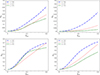Fig. E.1. X-ray polarization degree, ΠX = Πpp = 2.3 (top panels) and optical polarization degree, ΠO = Πpe = 4.6 (bottom panels) as a function of the viewing angle, θobs, which is expressed in radians. In the left panels the proper number density is assumed to be constant, whereas in the right panels the magnetization is assumed to be constant. The width of the proton emission region is assumed to be Δz = 3z0.

All Tables

All Figures

Fig. 1. Sketch of the scenario discussed in the text. The jet has a parabolic shape and carries a helical magnetic field. Particles are accelerated at some distance (z0) from the black hole. Electrons, which have a very short cooling time, produce the optical emission in a thin shell close to the acceleration zone. Protons, instead, are in the slow-cooling regime and are advected by the flow up to a distance Δz ∼ z0 (determined by the adiabatic energy losses). Protons produce the high-energy component of the SED, including the X-rays.

In the text

Fig. 2. X-ray polarization degree, ΠX (top panels) and chromaticity, ΠO/ΠX (bottom panels) as a function of the width of the proton emission region, Δz. In the left panels, the proper number density is assumed to be constant, whereas in the right panels, the magnetization is assumed to be constant. The X-ray polarization degree is ΠX = Πpp = 2.3, and the optical polarization degree is ΠO = Πpe = 4.6. The viewing angle is assumed to be θobs = 0.1 rad.

In the text

Fig. E.1. X-ray polarization degree, ΠX = Πpp = 2.3 (top panels) and optical polarization degree, ΠO = Πpe = 4.6 (bottom panels) as a function of the viewing angle, θobs, which is expressed in radians. In the left panels the proper number density is assumed to be constant, whereas in the right panels the magnetization is assumed to be constant. The width of the proton emission region is assumed to be Δz = 3z0.

In the text

References

- Abdo, A. A., Ackermann, M., Agudo, I., et al. 2010, ApJ, 716, 30 [NASA ADS] [CrossRef] [Google Scholar]
- Agudo, I., Liodakis, I., Otero-Santos, J., et al. 2025, ArXiv e-prints [arXiv:2505.01832] [Google Scholar]
- Aharonian, F. A. 2000, New Astron., 5, 377 [NASA ADS] [CrossRef] [Google Scholar]
- Bandiera, R., & Petruk, O. 2016, MNRAS, 459, 178 [NASA ADS] [CrossRef] [Google Scholar]
- Bandiera, R., & Petruk, O. 2024, A&A, 689, A137 [NASA ADS] [CrossRef] [EDP Sciences] [Google Scholar]
- Blandford, R., Meier, D., & Readhead, A. 2019, ARA&A, 57, 467 [NASA ADS] [CrossRef] [Google Scholar]
- Bolis, F., Sobacchi, E., & Tavecchio, F. 2024a, A&A, 690, A14 [NASA ADS] [CrossRef] [EDP Sciences] [Google Scholar]
- Bolis, F., Sobacchi, E., & Tavecchio, F. 2024b, Phys. Rev. D, 110, 123032 [Google Scholar]
- Bonometto, S., & Saggion, A. 1973, A&A, 23, 9 [Google Scholar]
- Böttcher, M. 2019, Galaxies, 7, 20 [Google Scholar]
- Capetti, A., Raiteri, C. M., & Buttiglione, S. 2010, A&A, 516, A59 [NASA ADS] [CrossRef] [EDP Sciences] [Google Scholar]
- Del Zanna, L., Volpi, D., Amato, E., & Bucciantini, N. 2006, A&A, 453, 621 [NASA ADS] [CrossRef] [EDP Sciences] [Google Scholar]
- Di Gesu, L., Marshall, H. L., Ehlert, S. R., et al. 2023, Nat. Astron., 7, 1245 [NASA ADS] [CrossRef] [Google Scholar]
- Fossati, G., Maraschi, L., Celotti, A., Comastri, A., & Ghisellini, G. 1998, MNRAS, 299, 433 [Google Scholar]
- Ghisellini, G., Celotti, A., Fossati, G., Maraschi, L., & Comastri, A. 1998, MNRAS, 301, 451 [NASA ADS] [CrossRef] [Google Scholar]
- Hillas, A. M. 1984, ARA&A, 22, 425 [Google Scholar]
- Krawczynski, H. 2012, ApJ, 744, 30 [NASA ADS] [CrossRef] [Google Scholar]
- Liodakis, I., & Petropoulou, M. 2020, ApJ, 893, L20 [Google Scholar]
- Liodakis, I., Zhang, H., Boula, S., et al. 2025, ArXiv e-prints [arXiv:2505.13603] [Google Scholar]
- Lyubarsky, Y. 2009, ApJ, 698, 1570 [NASA ADS] [CrossRef] [Google Scholar]
- Lyutikov, M., Pariev, V. I., & Blandford, R. D. 2003, ApJ, 597, 998 [Google Scholar]
- Marshall, H. L., Liodakis, I., Marscher, A. P., et al. 2024, ApJ, 972, 74 [NASA ADS] [CrossRef] [Google Scholar]
- Middei, R., Liodakis, I., Perri, M., et al. 2023, ApJ, 942, L10 [NASA ADS] [CrossRef] [Google Scholar]
- Murase, K., Dermer, C. D., Takami, H., & Migliori, G. 2012, ApJ, 749, 63 [Google Scholar]
- Pacciani, L., Kim, D. E., Middei, R., et al. 2025, ApJ, 983, 78 [Google Scholar]
- Peirson, A. L., Liodakis, I., & Romani, R. W. 2022, ApJ, 931, 59 [CrossRef] [Google Scholar]
- Peirson, A. L., Negro, M., Liodakis, I., et al. 2023, ApJ, 948, L25 [NASA ADS] [CrossRef] [Google Scholar]
- Poutanen, J. 1994, ApJS, 92, 607 [NASA ADS] [CrossRef] [Google Scholar]
- Romero, G. E., Boettcher, M., Markoff, S., & Tavecchio, F. 2017, Space Sci. Rev., 207, 5 [NASA ADS] [CrossRef] [Google Scholar]
- Sikora, M., Begelman, M. C., & Rees, M. J. 1994, ApJ, 421, 153 [Google Scholar]
- Sol, H., & Zech, A. 2022, Galaxies, 10, 105 [NASA ADS] [CrossRef] [Google Scholar]
- Tavecchio, F., Ghisellini, G., & Celotti, A. 2003, A&A, 403, 83 [NASA ADS] [CrossRef] [EDP Sciences] [Google Scholar]
- Tomsick, J., & COSI Collaboration 2022, in 37th International Cosmic Ray Conference, 652 [Google Scholar]
- Vlahakis, N. 2004, ApJ, 600, 324 [NASA ADS] [CrossRef] [Google Scholar]
- Webb, G. M. 1989, ApJ, 340, 1112 [Google Scholar]
- Weisskopf, M. C., Soffitta, P., Baldini, L., et al. 2022, J. Astron. Telescopes Instrum. Syst., 8, 026002 [NASA ADS] [Google Scholar]
- Zdziarski, A. A., & Bottcher, M. 2015, MNRAS, 450, L21 [NASA ADS] [CrossRef] [Google Scholar]
- Zech, A., Cerruti, M., & Mazin, D. 2017, A&A, 602, A25 [NASA ADS] [CrossRef] [EDP Sciences] [Google Scholar]
- Zhang, H. 2017, Galaxies, 5, 32 [Google Scholar]
- Zhang, H., & Böttcher, M. 2013, ApJ, 774, 18 [NASA ADS] [CrossRef] [Google Scholar]