| Issue |
A&A
Volume 701, September 2025
|
|
|---|---|---|
| Article Number | A220 | |
| Number of page(s) | 8 | |
| Section | Cosmology (including clusters of galaxies) | |
| DOI | https://doi.org/10.1051/0004-6361/202553824 | |
| Published online | 17 September 2025 | |
Determining H0 from a distance sum rule that combines gamma-ray bursts with observational Hubble data and strong gravitational lensing
1
Università di Camerino, Divisione di Fisica, Via Madonna delle Carceri 9, 62032 Camerino, Italy
2
SUNY Polytechnic Institute, 13502 Utica, New York, USA
3
INAF – Osservatorio Astronomico di Brera, Milano, Italy
4
INFN, Sezione di Perugia, Perugia, 06123
Italy
5
Al-Farabi Kazakh National University, Al-Farabi Av. 71, 050040 Almaty, Kazakhstan
6
ICRANet, Piazza della Repubblica 10, Pescara, 65122
Italy
⋆ Corresponding authors: This email address is being protected from spambots. You need JavaScript enabled to view it.
; This email address is being protected from spambots. You need JavaScript enabled to view it.
Received:
20
January
2025
Accepted:
5
May
2025
Abstract
Context. Model-independent bounds on the Hubble constant H0 are important for gaining insight into cosmological tensions.
Aims. We work out a model-independent analysis based on the sum rule, which is applied to late- and early-time data catalogs to determine H0.
Methods. Through the model-independent Bézier interpolation of the observational Hubble data and assuming a flat universe, we reconstructed the dimensionless distances of the sum rule and applied them to strong lensing data to derive constraints on H0. We then extended this method to the high-redshift domain, and in two separate analyses, we included gamma-ray burst (GRB) data sets from the well-established Amati and Combo correlations.
Results. In all three analyses, our findings agree at the 1σ level with the H0 determined from type Ia supernovae (SNe Ia), and at the 2σ level, our findings agree with the measurement derived from the cosmic microwave background (CMB) radiation.
Conclusions. Our method evidences that the bounds on H0 are significantly affected by strong lensing data, which favor the local measurement from SNe Ia. Including GRBs causes only a negligible decrease in the value of H0. This may indicate that GRBs can be used to trace the expansion history, and in conjunction with CMB measurements, GRBs may reconcile the Hubble tension and accommodate the flat ΛCDM paradigm purported by CMB data.
Key words: cosmological parameters / cosmology: miscellaneous / cosmology: observations / cosmology: theory / dark energy / large-scale structure of Universe
© The Authors 2025
 Open Access article, published by EDP Sciences, under the terms of the Creative Commons Attribution License (https://creativecommons.org/licenses/by/4.0), which permits unrestricted use, distribution, and reproduction in any medium, provided the original work is properly cited.
This article is published in open access under the Subscribe to Open model. This email address is being protected from spambots. You need JavaScript enabled to view it. to support open access publication.
1. Introduction
The Hubble constant H0 defines the current expansion rate of the Universe and is one of the most crucial cosmological parameters to measure. It represents the zeroth term in any cosmographic expansion (see, e.g., Aviles et al. 2012, 2017; Dunsby & Luongo 2016) and, in fact, cosmology was primarily focused on determining H0 and q0, the deceleration parameter (Sandage 1970), albeit the need of extending the analysis to higher orders has become increasingly evident (see, e.g., Neben & Turner 2013; Luongo 2013).
Despite its critical role in cosmology, current H0 bounds differ significantly, highlighting a persistent and still unresolved tension, possibly related to the emergence of new physics (Hu et al. 2024) or to some unexpected physical process and/or mechanism (Vagnozzi 2020). Nevertheless, the standard ΛCDM cosmological model, based on a bare cosmological constant Λ that describes dark energy, is currently criticized since recent results from DESI Collaboration (2025) may favor a mildly evolving scalar field, even at the level of background cosmology, thus pushing up the Universe to accelerate through a repulsive effect over standard gravity (Luongo & Quevedo 2014, 2018). However, several criticisms have been raised immediately after the release of their preliminary results (see, e.g., Ó Colgáin et al. 2026; Luongo & Muccino 2024; Carloni et al. 2025).
Using the ΛCDM model, bounds on H0 seem to agree with those from the Planck satellite; that is, they are deeply in tension with those found from type Ia supernovae (SNe Ia)1. In view of such results, better understanding of the ΛCDM drawbacks and inferring new strategies to constrain H0 appear extremely necessary in precision cosmology (Capozziello et al. 2022; Wolf et al. 2025; Adil et al. 2024; Ó Colgáin et al. 2022b, 2024, 2022a; Luongo et al. 2015), and consequently, fixing the spatial geometry density parameter, Ωk, may lead to unexpected inconsistency, for example, a higher lensing amplitude in the cosmic microwave background (CMB) power spectra (Planck Collaboration VI 2020).
The Hubble constant can be determined from time delay measurements of gravitationally lensed supernovae (Refsdal 1964), and such a data set can be expanded to include lensed quasars since their brightness and variable nature can be used to measure the so-called time-delay distance (Kelly et al. 2015; Goobar et al. 2017). This distance represents a combination of three angular diameter distances among the observer, lens, and source, but it suffers from the unsolved issue of “strong model dependence”2. Relaxing dark energy so that it does not behave as a constant would in fact imply severe departures from measuring H0, and in general, the role of spatial curvature significantly influences every background theory different from general relativity (see, e.g., Capozziello et al. 2018, 2019).
Fully model-independent treatments to determine H0 and/or Ωk are thus still the object of impressive efforts, and in this respect, the “distance sum rule” offers an effective method to determine the spatial curvature and the Hubble constant without relying on a specific cosmological model (Rasanen et al. 2015). Within this framework, significant efforts have been made in recent studies to constrain the cosmic curvature (Qi et al. 2019a; Wang et al. 2020; Xia et al. 2017; Li et al. 2018; Zhou & Li 2020). These studies utilized precise measurements of the source-lens/observer distance ratio in strong gravitational lensing (SGL) systems (Cao et al. 2015; Chen et al. 2019) as well as luminosity distances derived from various other distance indicators (Qi et al. 2019b; Liao 2019). However, this methodology is only weakly dependent on the Hubble constant, as H0 enters not through a direct distance measurement but rather through a distance ratio (Cao et al. 2012). It is worth noting that for effective implementation of the distance sum rule, utilizing distance probes at higher redshifts would be advantageous, as this would enrich the sample of SGL points with alternative catalogs.
Motivated by the above considerations, in this paper, we consider the sum rule in order to constrain the Hubble constant, including high-redshift data points and adopting a model-independent treatment to describe the Hubble rate at different redshifts. To do so, we employed gamma-ray bursts (GRBs) as high-redshift distance indicators, adding the observational Hubble rate data (OHD), directly measured at different redshifts, together with data from the SGL of quasars. In this respect, we identify two GRB correlations as being the most promising, namely the Ep − Eiso (or Amati) and L0 − Ep − T (or Combo) correlations, while fixing the background through the use of the model-independent Bézier polynomials. The latter is a technique that approximates the Hubble rate up to the redshifts of our interest, thus avoiding de facto postulation of the dark energy model (see Amati et al. 2019). In our treatment, we force a vanishing spatial curvature in order to avoid model dependence on the cosmic parameters in the distance determination. Accordingly, we performed three analyses: the first combines OHD and SGL catalogs, the second includes the high-redshift GRB data from the Ep − Eiso correlation, and in the third, the L0 − Ep − T correlation replaces the Ep − Eiso correlation. Each analysis is based on the Markov chain Monte Carlo (MCMC) method and the Metropolis-Hastings algorithm, run by modifying the free Wolfram Mathematica code presented in Arjona et al. (2019).
Our findings indicate H0 is close to the local value inferred by Riess et al. (2019), in agreement with the expectations coming from lensed quasars. Accordingly, we discuss the Hubble tension, and we compare our findings with Planck Collaboration VI (2020). The implications of our findings for dark energy evolutions show that the standard cosmological background is well approximated by a flat ΛCDM model, thus agreeing with the most recent developments (Luongo & Muccino 2024; Carloni et al. 2025) that criticize the preliminary results obtained by DESI Collaboration (2025), which instead suggest a slightly varying dark energy evolution.
This paper is structured as follows. In Sect. 2, we introduce our methodology, which is based on the Bézier polynomial interpolation and the sum rule, GRB correlations, and OHD and lensed data catalogs. In Sect. 3, the three MCMC analyses and their corresponding results are shown. Finally, in Sect. 4 we discuss developments, physical interpretation, and perspectives of our work.
2. Methods and cosmic data sets
Considering the validity of the cosmological principle3, the corresponding maximally symmetric spacetime well describing the Universe is the Friedmann-Robertson-Walker (FRW) metric. Accordingly, the comoving distance of a source at redshift zs with emission time ts as seen by an observer at redshift zl characterized by a time tl > ts at which the observation is performed is defined by
![Mathematical equation: $$ \begin{aligned} d_M(z_l,z_s) = \frac{c}{H_0\sqrt{\Omega _k}}\sinh {\left[\int ^{z_s}_{z_l} \frac{H_0\sqrt{\Omega _k}}{H(z\prime )} \mathrm{d}z\prime \right]}. \end{aligned} $$](/articles/aa/full_html/2025/09/aa53824-25/aa53824-25-eq1.gif) (1)
(1)
Here, c is the speed of light.
Conveniently, introducing the dimensionless comoving distance, d = H0dM/c, and defining
 (2a)
(2a)
 (2b)
(2b)
 (2c)
(2c)
from Eq. (1), we derive the well-known “distance sum rule”, for a generic non-flat FRW Universe (Rasanen et al. 2015):
 (3)
(3)
which appears as a ratio among distances defined in Eqs. (2a)–(2c).
Hence, knowing dl and ds enables one to place constraints on Ωk (Qi et al. 2019b) and test the validity of the FRW metric (Qi et al. 2019a; Cao et al. 2019).
Accordingly, Eq. (3) can be also written as
 (4)
(4)
Now, the difference with respect to Eq. (3) is that the ratio dlds/dls defines a (dimensionless) distance.
If we measure dl and ds and we know the above ratio from an observable in terms of dimensional distances, then Eq. (4) can also be used to constrain H0.
2.1. Dimensionless distances from OHD
The OHD catalog (Luongo & Muccino 2025) consists of NO = 34 measurements Hk of the Hubble rate obtained by considering passively evolving galaxies at various redshifts z as cosmic chronometers. Assuming that all stars formed at the same time, Δt, in these galaxies, through their spectroscopic redshift measurements, the Hubble rate is derived as H(z)≃ − (1 + z)−1(Δz/Δt) (Jimenez & Loeb 2002; Moresco et al. 2022).
Hence, the catalog can be interpolated by the well-established second-order Bézier curve (Amati et al. 2019; Luongo & Muccino 2021a, 2023, 2025; Montiel et al. 2021; Muccino et al. 2023; Alfano et al. 2024a,b,c):
![Mathematical equation: $$ \begin{aligned} \mathcal{H} (z) = \frac{\alpha _\star }{z_{\rm m}^2} \left[\alpha _0(z_{\rm m}-z)^2 + 2\alpha _1 z(z_{\rm m}-z) +\alpha _2 z^2\right], \end{aligned} $$](/articles/aa/full_html/2025/09/aa53824-25/aa53824-25-eq7.gif) (5)
(5)
where α⋆ = 100 km s−1 Mpc−1 is a normalization, αi are the Bézier coefficients, and zm = 1.965 is the largest redshift of the OHD catalog. At z = 0 from Eq. (5), we defined the dimensionless Hubble constant as h0 ≡ H0/α⋆ ≡ α0.
Although Eq. (5) is model independent, the reconstructed d(z) is independent from any cosmological parameters only if assuming a zero spatial curvature:
 (6)
(6)
In view of this assumption, we considered Eqs. (3) and (4) with Ωk ≡ 0. Thus, in the following analyses, we focus only on the determination of the Hubble constant. It is worth emphasizing that the Bézier parametric interpolation has significant advantages over other non-parametric interpolation methods, such as the Gaussian process (see, e.g., Melia & Yennapureddy 2018) or machine learning (see, e.g., Bengaly et al. 2023). Namely, Eq. (6) has an analytical expression that greatly reduces the computational time, and the α0 parameter provides immediate information on the Hubble constant.
2.2. Constraints at high redshifts with GRBs
Correlations have been proposed as tools to standardize GRBs and probe the Universe up to z ∼ 8 − 9 (Amati & Della Valle 2013; Yonetoku et al. 2004; Ghirlanda et al. 2004; Muccino et al. 2021; Luongo & Muccino 2021b; Cao et al. 2022). We used two well-consolidated correlations.
The first is the Amati or Ep − Eiso correlation. This is a prompt emission correlation expressed as (Amati & Della Valle 2013)
 (7)
(7)
with intercept a and slope b. It correlates the rest-frame peak energy Ep (in kiloelectronvolt units) of the γ-ray energy spectrum with the isotropic radiated energy Eiso (in erg units) integrated over the total duration of the burst, and it is defined as (Luongo & Muccino 2021b)
![Mathematical equation: $$ \begin{aligned} E_{\rm iso} = 4\pi \left[d_L^A(z)\right]^2{S\!}_b(1+z)^{-1}. \end{aligned} $$](/articles/aa/full_html/2025/09/aa53824-25/aa53824-25-eq10.gif) (8)
(8)
Here, Sb (in erg cm2 units) is the observed bolometric fluence in the rest-frame 1 − 104 keV band. The correlation is also characterized by a dispersion parameter, σ, that accounts for systematics and additional hidden uncertainties.
From Eqs. (7) and (8), the luminosity distance dL(z) = c(1 + z)d(z)/H0 can be expressed as
![Mathematical equation: $$ \begin{aligned} \log {d_L^A} = \frac{1}{2}\left[\frac{\log {E_{\rm p}}-a}{b} - \log {\left(\frac{{S\!}_b}{1+z}\right)}\right]+d_0^A, \end{aligned} $$](/articles/aa/full_html/2025/09/aa53824-25/aa53824-25-eq11.gif) (9)
(9)
where d0A = 0.96 includes all the constants and the conversion factor from centimeter to megaparsec.
The second is the Combo or L0 − Ep − T correlation. It is a hybrid prompt-afterglow correlation (Muccino et al. 2021):
 (10)
(10)
with intercept a and slope b. It correlates the prompt observable Ep (in kiloelectronvolt units) with the 0.3 − 10 keV rest-frame X-ray afterglow luminosity L0 (in erg s−1 units) and the effective rest-frame duration T (in seconds) of the plateau phase (Luongo & Muccino 2021b). The term L0 is related to the rest-frame 0.3 − 10 keV plateau flux, F0 (in erg cm2 s−1 units), through
![Mathematical equation: $$ \begin{aligned} L_0=4\pi \left[d^C_L(z)\right]^2 F_0. \end{aligned} $$](/articles/aa/full_html/2025/09/aa53824-25/aa53824-25-eq13.gif) (11)
(11)
Also, this correlation is endowed by a scatter, σ.
From Eqs. (10) and (11), the luminosity distance reads as
![Mathematical equation: $$ \begin{aligned} \log {d^C_L} = \frac{1}{2}\left[a + b\log {E_{\rm p}} - \log {T} - \log {F_0}\right]+d_0^C, \end{aligned} $$](/articles/aa/full_html/2025/09/aa53824-25/aa53824-25-eq14.gif) (12)
(12)
where d0C = −25.04 includes all the constants and the conversion factor from centimeter to megaparsec.
Equations (9) and (12) can be separately compared with Eq. (6) to extend the d − z diagram to z ∼ 8 − 9, but this requires constraining the correlation parameters (a, b, and σ for each correlation).
In our analyses, we considered the most updated and refined catalogs composed of NA = 118 sources for the Ep − Eiso correlation (Khadka et al. 2021) and NC = 174 bursts for the L0 − Ep − T correlation (Muccino et al. 2021).
2.3. Time-delay measurements from lensed quasars
In an SGL system, as the source and an early-type galaxy act as the lens, the time delays, Δtij, between lensed images i and j and the gravitational potential of the lensing galaxy, Δϕij, are related via the time-delay distance, D, (Qi et al. 2021):
 (13)
(13)
Using the definition D ≡ (1 + zl)dA, ldA, s/dA, ls, where dA(z) = cd(z)/[H0(1 + z)] is the angular distance, one can interpolate the time-delay distance (Qi et al. 2021):
 (14)
(14)
We considered NL = 7 precise determinations of D from SGL quasar-galaxy systems B1608+656, RX J1131−1231, HE 0435−1223, SDSS 1206+4332, WFI2033−4723, and PG 1115+080, released by the H0LiCOW collaboration (Wong et al. 2020), and DES J0408−5354, released by the STRIDES collaboration (Shajib et al. 2020). All sources cover the range zs ∈ [0.654, 2.375].
2.4. Applying the sum rule to the combined catalogs
Strong gravitational lensing systems provide unique measurements of D that can be related to the corresponding interpolated time-delay distances 𝒟 given by Eq. (14). We note that 𝒟 depends on the ratio dlds/dls, which is intimately related to the distance sum rule in Eq. (4), and it can be determined only if we are able to measure the dimensionless distances dl and ds.
To this aim, the fundamental role of the OHD catalog, through its interpolation of the Hubble rate via Eq. (5), consists of providing model-independent estimates of dl and ds via Eq. (6). Therefore, combining SGL and OHD catalogs through Eqs. (4), (6), and (14) allows us to infer the value of H0 or h0 ≡ α0 from the distance sum rule without involving a priori cosmological models.
Finally, we may get further constraints on H0 by extending the d − z diagram to z ∼ 8 − 9 through the inclusion of GRB data sets from Ep − Eiso and L0 − Ep − T correlations. To do so, we would need to compare the corresponding luminosity distances – given by Eqs. (9) and (12), respectively – with the interpolated log[c(1 + z)d(z)/(α⋆α0)] obtained from Eq. (6). As mentioned above, including GRBs requires additional parameters (a, b, and σ for each correlation) to be constrained.
3. MCMC analyses and results
We performed three analyses: MCMC 1, which considers only low-redshift catalogs (i.e., OHD and SGL); MCMC 2, which includes the Ep − Eiso catalog in addition to OHD and SGL data; and MCMC 3, which utilizes the L0 − Ep − T catalog instead of the Ep − Eiso one. These analyses do not introduce a hierarchy among the free coefficients or data sets. Rather, their purpose is to show the differences in the numerical outcomes once late- and early-time catalogs of data points are included. Below we describe for each MCMC procedure the corresponding fitting functions and bounds.
3.1. MCMC 1 outcomes
To determine the dimensionless distances ds and dl, we needed to estimate the best-fit parameters α0 ≡ h0, α1, and α2. This was done by using the OHD catalog and maximizing the log-likelihood function
![Mathematical equation: $$ \begin{aligned} \ln \mathcal{L} _O = -\frac{1}{2} \sum ^{N_O}_{k=1} \left\{ \ln \left(2\pi \sigma ^2_{H_k}\right) + \left[\frac{H_k-\mathcal{H} (z_k)}{\sigma _{H_k}}\right]^2\right\} , \end{aligned} $$](/articles/aa/full_html/2025/09/aa53824-25/aa53824-25-eq17.gif) (15)
(15)
where σHk are the errors attached to Hk. To strengthen the constraint on α0 ≡ h0, we employed the SGL data set. In this case, the best-fit parameters are determined by maximizing the following log-likelihood function:
![Mathematical equation: $$ \begin{aligned} \ln \mathcal{L} _L = -\frac{1}{2} \sum ^{N_L}_{k=1} \left\{ \ln \left(2\pi \sigma ^2_{D_k}\right) + \left[\frac{D_k-\mathcal{D} (z_k)}{\sigma _{D_k}}\right]^2\right\} , \end{aligned} $$](/articles/aa/full_html/2025/09/aa53824-25/aa53824-25-eq18.gif) (16)
(16)
where σDk are the errors attached to Dk.
Hence, joint constraints from OHD and SGL catalogs can be obtained by maximizing the combined log-likelihoodfunction
 (17)
(17)
The results are summarized in Table 1 and displayed in Fig. 1. We immediately noticed that the inclusion of SGL data provides Bézier coefficients αi with attached errors larger than those obtained by considering OHD only (Amati et al. 2019; Luongo & Muccino 2021a, 2023, 2025; Montiel et al. 2021; Muccino et al. 2023; Alfano et al. 2024a,b,c). Moreover, while α1 and α2 are in line with those obtained by considering OHD only, the lowest-order coefficient α0 ≡ h0 shifted from the usual value of α0 ≃ 0.67 − 0.69 (Amati et al. 2019; Luongo & Muccino 2021a, 2023, 2025; Montiel et al. 2021; Muccino et al. 2023; Alfano et al. 2024a,b,c) to a higher value of α0 ≃ 0.76, which is consistent with the results based on SGL data applied to the distance sum rule (for a comparison with the same assumption Ωk = 0, see the SGL entry in Table 1 andQi et al. 2021).
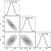 |
Fig. 1. MCMC 1 contour plots. Darker (lighter) areas display 1σ (2σ) confidence regions. |
Comparison of the best-fit among the MCMC 1, MCMC 2, and MCMC 3 analyses and separate constraints of SGL and OHD.
To single out the effect of the SGL catalog on the estimate of h0, we performed two additional checks involving only the OHD catalog: OHD 1, from which we extracted the best-fit coefficients αi of the Bézier interpolation, and OHD 2, which considers the Hubble rate of the flat ΛCDM model  . The results of the OHD 1 and 2 checks are reported in Table 1. It was immediately clear that the constraint on h0 from the Bézier polynomial interpolation is fully consistent with the ΛCDM expectation. This implies that the high h0 in Table 1 inferred for the MCMC 1 analysis (but also for the MCMC 2 and 3 analyses, as we show in the following) is driven by SGL data (Qi et al. 2021).
The reason behind the significant influence of SGL data on the Hubble constant determination is genuinely due to the relative errors of SGL (Qi et al. 2021) and OHD (Alfano et al. 2024a,b,c) catalogs: the relative errors for the SGL data are in the range 4 − 9%, whereas for the OHD catalog the range is 5 − 65%; focusing on the relative errors of the lowest-redshift data points, for SGL data stay at 4%, whereas for the OHD data are at 34%. Naively speaking, if we look at the estimate of h0 as a weighted average over the values obtained from SGL and OHD catalogs, the result tends to lean toward the value with the least (relative) error.
3.2. MCMC 2 outcomes
Next, we included the GRBs of the Ep − Eiso data set to check to what extent the Bézier coefficients, in particular α0, are affected by extending the d − z diagram to z ∼ 8 − 9. It is worth noting that the inclusion of this data set introduces additional free parameters (a, b, and σ) to be evaluated, possibly deteriorating the best-fit accuracy.
The log-likelihood for the GRBs of the Ep − Eiso (or Amati) correlation is given by
![Mathematical equation: $$ \begin{aligned} \ln \mathcal{L} _A =&-\frac{1}{2} \sum ^{N_A}_{k=1} \left\{ \frac{\log {[c(1+z_k) d_k/(\alpha _\star \alpha _0)]} -\log {d^A_{L,k}}}{\sigma _{\log {d^A_{L,k}}}}\right\} ^2\nonumber \\&-\frac{1}{2} \sum ^{N_A}_{k=1} \ln \left(2\pi \sigma ^2_{\log {d^A_{L,k}}}\right), \end{aligned} $$](/articles/aa/full_html/2025/09/aa53824-25/aa53824-25-eq41.gif) (18)
(18)
where dk is defined in Eq. (6) and log dL, kA in Eq. (9), whereas the errors on log dL, k are defined as
 (19)
(19)
The best-fit Bézier coefficients αi and the correlation parameters a, b, and σ are thus obtained by maximizing the combinedlog-likelihood function
 (20)
(20)
The results are summarized in Table 1 and displayed in Fig. 2. With respect to MCMC 1, the inclusion of GRB data does not significantly change the Bézier best-fit coefficients, αi, nor increase the attached errors. The value of α0 ≡ h0 has slightly decreased with respect to the MCMC 1 analysis, but it is still high (α0 ≃ 0.75) and again significantly influenced by SGL data (Qi et al. 2021). Regarding the Ep − Eiso correlation parameters, their values are in line with those obtained by calibrating this correlation with the OHD catalog (Amati et al. 2019; Luongo & Muccino 2021a, 2023; Montiel et al. 2021; Muccino et al. 2023; Alfano et al. 2024a,b,c).
 |
Fig. 2. MCMC 2 contour plots. Darker (lighter) areas display the 1σ (2σ) confidence regions. |
3.3. MCMC 3 outcomes
Here, we consider the GRBs from the L0 − Ep − T correlation. The general implications of adding a GRB catalog that requires the fitting of additional parameters still hold for this case. As with the previous case, the log-likelihood for the GRBs of the L0 − Ep − T (or Combo) correlation isgiven by
![Mathematical equation: $$ \begin{aligned} \ln \mathcal{L} _C =&-\frac{1}{2} \sum ^{N_C}_{k=1} \left\{ \frac{\log {[c(1+z_k) d_k/(\alpha _\star \alpha _0)]} -\log {d^C_{L,k}}}{\sigma _{\log {d^C_{L,k}}}}\right\} ^2\nonumber \\&-\frac{1}{2} \sum ^{N_C}_{k=1} \ln \left(2\pi \sigma ^2_{\log {d^C_{L,k}}}\right), \end{aligned} $$](/articles/aa/full_html/2025/09/aa53824-25/aa53824-25-eq44.gif) (21)
(21)
where dk is again defined by Eq. (6), but log dL, k is now given by Eq. (12). The corresponding errors are
 (22)
(22)
In this case, αi, a, b, and σ are obtained by maximizing the combined log-likelihood function
 (23)
(23)
The corresponding results are summarized in Table 1 and displayed in Fig. 3.
 |
Fig. 3. MCMC 3 contour plots. Darker (lighter) areas display 1σ (2σ) confidence regions. |
Changing the GRB data set leads to results similar to the those of the MCMC 2 analysis, both in terms of Bézier coefficients and correlation parameters. Basically, the most noteworthy conclusions from the MCMC 3 analysis are that (i) the value of α0 ≡ h0 is (again) significantly influenced by SGL data (Qi et al. 2021), and (ii) the L0 − Ep − T correlation is characterized by a very small dispersion, when compared to the Ep − Eiso correlation.
4. Final outlook
Within model-independent reconstruction techniques, we have focused on determining H0 bounds in order to better understand the cosmological tension by reconciling late- and early-time data. To do so, we worked out a model-independent analysis involving the so-called sum rule, for which we selected late- and early-time data catalogs to estimate the Universe’s expansion rate today. More precisely, we interpolated the most recent OHD catalog via a Bézier second-order function without dependence on a model. In this respect, the Bézier polynomials were able to frame the Universe dynamics similarly to splines, i.e., constructing a test function that is not based on the sum of cosmic fluids, as happens for dark energy models. Further, to obtain model-independent determinations of the dimensionless distance from OHD and reconcile observations made at our time with the ones at high redshifts from GRBs, we assumed the Universe to be flat (i.e., Ωk = 0).
We performed three analyses. In the first one, named MCMC 1, we employed only low-redshift catalogs, namely OHD, to reconstruct the dimensionless distances, combined them into the distance sum rule, and applied them directly to SGL data. In the second and third analyses, respectively MCMC 2 and 3, we extended our approach to the high-redshift regime, incorporating within two separate analyses two GRB correlation data sets, namely the Ep − Eiso correlation for MCMC 2 and the L0 − Ep − T correlation for MCMC 3. In all the aforementioned cases, we performed an MCMC analysis based on the Metropolis-Hastings algorithm. We derived constraints on H0 that are consistent at the 1σ level with the local measurement of H0 obtained by Riess et al. (2019) from SNe Ia. Quite unexpectedly, however, the agreement is only at the 2σ level with the measurement based on the CMB radiation (Planck Collaboration VI 2020).
Our findings highlight the significant influence of SGL data, which agree more closely with the local supernova measurements on H0. Moreover, our results show that the inclusion of GRB data furnishes a minimal impact on determining H0, likely indicating that GRBs could serve as effective probes of the expansion history and, at the same time, that it is possible that the Hubble tension may be due to the need of reconciling early- and late-time data rather than indicating new physics4. Moreover, combined with the CMB radiation data, GRBs might help alleviate the Hubble tension while remaining compatible with the flat ΛCDM paradigm.
Future works will be devoted to exploring the following avenues: the influence of SGL data on cosmic probes, the inclusion of high-redshift data inferred from GRBs, and possibly testing again the dark energy models adopting generic lensing data and the sum rule. Also of interest would be verifying how and whether the current expectations obtained from international collaborations, such as DESI, Planck, and the future Euclid missions, may be compared once they include such data catalogs and the use of the cosmic distance sum rule.
H0 = (67.4 ± 0.5) km s−1 Mpc−1 from Planck Collaboration VI (2020) and H0 = (74.03 ± 1.42) km s−1 Mpc−1 from Riess et al. (2019) yield a severe 4.4σ confidence level tension.
In other words, such measurements are jeopardized by the strong inconsistency of fixing the cosmological model a priori, implying very different results due to the fact that the right cosmological model is still under scrutiny, as its form appears quite unconstrained (Wolf & Ferreira 2023).
For an example of a recent criticism on this, see Luongo et al. (2022).
Usually, the inclusion of GRBs may lead to unexpectedly large determinations of mass (Muccino et al. 2021). Nevertheless, their use to constrain background cosmology may provide misleading results, due to the calibration procedure (Khadka et al. 2021). Accordingly, the combination of GRBs with low-redshift data catalogs may refine the analyses, suggesting possible deviations from the standard ΛCDM model (Luongo & Muccino 2020).
Acknowledgments
The authors express their gratitude for discussions to Deepak Jain about the topic of model-independent reconstructions in cosmology. OL is thankful to Sunny Vagnozzi for interactions in the field of cosmology and Hubble tension, during his stay at the University of Camerino. The authors acknowledge Giovanni delle Monache for private debates on the subjects of statistics, data analysis and their use in theoretical backgrounds.
References
- Adil, S. A., Akarsu, Ö., Malekjani, M., et al. 2024, MNRAS, 528, L20 [Google Scholar]
- Alfano, A. C., Capozziello, S., Luongo, O., & Muccino, M. 2024a, J. High Energy Astrophys., 42, 178 [NASA ADS] [CrossRef] [Google Scholar]
- Alfano, A. C., Luongo, O., & Muccino, M. 2024b, A&A, 686, A30 [NASA ADS] [CrossRef] [EDP Sciences] [Google Scholar]
- Alfano, A. C., Luongo, O., & Muccino, M. 2024c, J. Cosmol. Astropart. Phys., 2024, 055 [Google Scholar]
- Amati, L., & Della Valle, M. 2013, IJMPD, 22, 1330028 [Google Scholar]
- Amati, L., D’Agostino, R., Luongo, O., Muccino, M., & Tantalo, M. 2019, MNRAS, 486, L46 [CrossRef] [Google Scholar]
- Arjona, R., Cardona, W., & Nesseris, S. 2019, Phys. Rev. D, 99, 043516 [NASA ADS] [CrossRef] [Google Scholar]
- Aviles, A., Gruber, C., Luongo, O., & Quevedo, H. 2012, Phys. Rev. D, 86, 123516 [CrossRef] [Google Scholar]
- Aviles, A., Klapp, J., & Luongo, O. 2017, Phys. Dark Univ., 17, 25 [Google Scholar]
- Bengaly, C., Dantas, M. A., Casarini, L., & Alcaniz, J. 2023, Eur. Phys. J. C, 83, 548 [Google Scholar]
- Cao, S., Pan, Y., Biesiada, M., Godlowski, W., & Zhu, Z. 2012, JCAP, 2012, 016 [CrossRef] [Google Scholar]
- Cao, S., Biesiada, M., Gavazzi, R., Piórkowska, A., & Zhu, Z.-H. 2015, ApJ, 806, 185 [NASA ADS] [CrossRef] [Google Scholar]
- Cao, S., Qi, J., Cao, Z., et al. 2019, Sci. Rep., 9, 11608 [NASA ADS] [CrossRef] [Google Scholar]
- Cao, S., Dainotti, M., & Ratra, B. 2022, MNRAS, 512, 439 [NASA ADS] [CrossRef] [Google Scholar]
- Capozziello, S., Luongo, O., Pincak, R., & Ravanpak, A. 2018, Gen. Relat. Grav., 50, 53 [Google Scholar]
- Capozziello, S., D’Agostino, R., & Luongo, O. 2019, IJMPD, 28, 1930016 [Google Scholar]
- Capozziello, S., D’Agostino, R., & Luongo, O. 2022, Phys. Dark Univ., 36, 101045 [Google Scholar]
- Carloni, Y., Luongo, O., & Muccino, M. 2025, Phys. Rev. D, 111, 023512 [Google Scholar]
- Chen, Y., Li, R., Shu, Y., & Cao, X. 2019, MNRAS, 488, 3745 [NASA ADS] [CrossRef] [Google Scholar]
- DESI Collaboration 2025, JCAP, 2025, 021 [Google Scholar]
- Dunsby, P. K. S., & Luongo, O. 2016, Int. J. Geometric Meth. Mod. Phys., 13, 1630002 [Google Scholar]
- Ghirlanda, G., Ghisellini, G., & Lazzati, D. 2004, ApJ, 616, 331 [Google Scholar]
- Goobar, A., Amanullah, R., Kulkarni, S. R., et al. 2017, Science, 356, 291 [Google Scholar]
- Hu, J. P., Jia, X. D., Hu, J., & Wang, F. Y. 2024, ApJ, 975, L36 [Google Scholar]
- Jimenez, R., & Loeb, A. 2002, ApJ, 573, 37 [NASA ADS] [CrossRef] [Google Scholar]
- Kelly, P. L., Rodney, S. A., Treu, T., et al. 2015, Science, 347, 1123 [Google Scholar]
- Khadka, N., Luongo, O., Muccino, M., & Ratra, B. 2021, JCAP, 2021, 042 [Google Scholar]
- Li, Z., Ding, X., Wang, G.-J., Liao, K., & Zhu, Z.-H. 2018, ApJ, 854, 146 [Google Scholar]
- Liao, K. 2019, Phys. Rev. D, 99, 083514 [NASA ADS] [CrossRef] [Google Scholar]
- Luongo, O. 2013, Mod. Phys. Lett. A, 28, 1350080 [NASA ADS] [CrossRef] [Google Scholar]
- Luongo, O., & Muccino, M. 2020, A&A, 641, A174 [NASA ADS] [CrossRef] [EDP Sciences] [Google Scholar]
- Luongo, O., & Muccino, M. 2021a, MNRAS, 503, 4581 [NASA ADS] [CrossRef] [Google Scholar]
- Luongo, O., & Muccino, M. 2021b, Galaxies, 9, 77 [NASA ADS] [CrossRef] [Google Scholar]
- Luongo, O., & Muccino, M. 2023, MNRAS, 518, 2247 [Google Scholar]
- Luongo, O., & Muccino, M. 2024, A&A, 690, A40 [NASA ADS] [CrossRef] [EDP Sciences] [Google Scholar]
- Luongo, O., & Muccino, M. 2025, A&A, 693, A187 [NASA ADS] [CrossRef] [EDP Sciences] [Google Scholar]
- Luongo, O., & Quevedo, H. 2014, Phys. Rev. D, 90, 084032 [Google Scholar]
- Luongo, O., & Quevedo, H. 2018, Found. Phys., 48, 17 [Google Scholar]
- Luongo, O., Battista Pisani, G., & Troisi, A. 2015, ArXiv e-prints [arXiv:1512.07076] [Google Scholar]
- Luongo, O., Muccino, M., Colgáin, E. Ó., Sheikh-Jabbari, M. M., & Yin, L. 2022, Phys. Rev. D, 105, 103510 [NASA ADS] [CrossRef] [Google Scholar]
- Melia, F., & Yennapureddy, M. K. 2018, JCAP, 2018, 034 [Google Scholar]
- Montiel, A., Cabrera, J. I., & Hidalgo, J. C. 2021, MNRAS, 501, 3515 [Google Scholar]
- Moresco, M., Amati, L., Amendola, L., et al. 2022, Liv. Rev. Relat., 25, 6 [NASA ADS] [Google Scholar]
- Muccino, M., Izzo, L., Luongo, O., et al. 2021, ApJ, 908, 181 [Google Scholar]
- Muccino, M., Luongo, O., & Jain, D. 2023, MNRAS, 523, 4938 [NASA ADS] [CrossRef] [Google Scholar]
- Neben, A. R., & Turner, M. S. 2013, ApJ, 769, 133 [Google Scholar]
- Ó Colgáin, E., Sheikh-Jabbari, M. M., Solomon, R., et al. 2022a, Phys. Rev. D, 106, L041301 [CrossRef] [Google Scholar]
- Ó Colgáin, E., Sheikh-Jabbari, M. M., & Solomon, R. 2022b, ArXiv e-prints [arXiv:2211.02129] [Google Scholar]
- Ó Colgáin, E., Sheikh-Jabbari, M. M., Solomon, R., Dainotti, M. G., & Stojkovic, D. 2024, Phys. Dark Univ., 44, 101464 [Google Scholar]
- Ó Colgáin, E., Dainotti, M. G., Capozziello, S., et al. 2026, J. High Energy Astrophys., 49, 100428 [Google Scholar]
- Planck Collaboration VI. 2020, A&A, 641, A6 [NASA ADS] [CrossRef] [EDP Sciences] [Google Scholar]
- Qi, J., Cao, S., Biesiada, M., et al. 2019a, Phys. Rev. D, 100, 023530 [NASA ADS] [CrossRef] [Google Scholar]
- Qi, J.-Z., Cao, S., Zhang, S., et al. 2019b, MNRAS, 483, 1104 [NASA ADS] [CrossRef] [Google Scholar]
- Qi, J.-Z., Zhao, J.-W., Cao, S., Biesiada, M., & Liu, Y. 2021, MNRAS, 503, 2179 [NASA ADS] [CrossRef] [Google Scholar]
- Rasanen, S., Bolejko, K., & Finoguenov, A. 2015, Phys. Rev. Lett., 115, 101301 [Google Scholar]
- Refsdal, S. 1964, MNRAS, 128, 307 [NASA ADS] [CrossRef] [Google Scholar]
- Riess, A. G., Casertano, S., Yuan, W., Macri, L. M., & Scolnic, D. 2019, ApJ, 876, 85 [Google Scholar]
- Sandage, A. R. 1970, Phys. Today, 23, 34 [Google Scholar]
- Shajib, A. J., Birrer, S., Treu, T., et al. 2020, MNRAS, 494, 6072 [Google Scholar]
- Vagnozzi, S. 2020, Phys. Rev. D, 102, 023518 [Google Scholar]
- Wang, B., Qi, J.-Z., Zhang, J.-F., & Zhang, X. 2020, ApJ, 898, 100 [NASA ADS] [CrossRef] [Google Scholar]
- Wolf, W. J., & Ferreira, P. G. 2023, Phys. Rev. D, 108, 103519 [NASA ADS] [CrossRef] [Google Scholar]
- Wolf, W. J., Ferreira, P. G., & García-García, C. 2025, Phys. Rev. D, 111, L041303 [Google Scholar]
- Wong, K. C., Suyu, S. H., Chen, G. C., et al. 2020, MNRAS, 498, 1420 [NASA ADS] [CrossRef] [Google Scholar]
- Xia, J.-Q., Yu, H., Wang, G.-J., et al. 2017, ApJ, 834, 75 [CrossRef] [Google Scholar]
- Yonetoku, D., Murakami, T., Nakamura, T., et al. 2004, ApJ, 609, 935 [Google Scholar]
- Zhou, H., & Li, Z.-X. 2020, ApJ, 899, 186 [Google Scholar]
All Tables
Comparison of the best-fit among the MCMC 1, MCMC 2, and MCMC 3 analyses and separate constraints of SGL and OHD.
All Figures
|
Fig. 1. MCMC 1 contour plots. Darker (lighter) areas display 1σ (2σ) confidence regions. |
| In the text | |
|
Fig. 2. MCMC 2 contour plots. Darker (lighter) areas display the 1σ (2σ) confidence regions. |
| In the text | |
|
Fig. 3. MCMC 3 contour plots. Darker (lighter) areas display 1σ (2σ) confidence regions. |
| In the text | |
Current usage metrics show cumulative count of Article Views (full-text article views including HTML views, PDF and ePub downloads, according to the available data) and Abstracts Views on Vision4Press platform.
Data correspond to usage on the plateform after 2015. The current usage metrics is available 48-96 hours after online publication and is updated daily on week days.
Initial download of the metrics may take a while.