© The Authors 2025

1 Introduction

Gravitational lensing has become one of the most important fields in present-day astronomy, largely driven by considerable improvements in observational capabilities. Its distinguished feature of being independent of the nature and physical state of the deflecting mass makes it perfectly suited to study dark matter in the Universe. In recent years, interest has increased in exploring the two most dominant components of the Universe: dark matter and dark energy. To this end, large-scale imaging and spectro-scopic surveys are currently being undertaken, such as those of the Euclid mission (Euclid Collaboration: Mellier et al. 2025), launched in July 2023, the Rubin Observatory (Legacy Survey of Space and Time; Brough et al. 2020), and the Roman Space Telescope (Spergel et al. 2015), set to begin in late 2025, which will map the sky with unprecedented accuracy. A prominent cos-mological probe for these surveys is weak gravitational lensing.

Weak gravitational lensing refers to the subtle distortions observed in the images of distant galaxies caused by the gravitational influence of massive structures along the line of sight. This phenomenon manifests in two primary ways: (i) a convergence field, κ, leads to the magnification or demagnification of the background galaxies’ images, altering their apparent size and brightness, and (ii) the shear, γ, stretches the galaxies’ shapes, causing them to appear more elliptical or skewed than they intrinsically are.

The convergence field, κ, cannot be observed directly due to the mass-sheet degeneracy (Bartelmann & Schneider 2001; Kilbinger 2015). Physically, it represents the projected total matter density along the line of sight, modulated by a lensing kernel in the mid-distance between the observer and the galaxy sources. A widely used mass-mapping algorithm is the Kaiser-Squires method (Kaiser & Squires 1993), which operates as a simple linear operator in Fourier space. However, this method has limitations, such as not accounting for missing data or the effect of noise.

In this paper we propose using a complex formalism for weak lensing, first introduced by Straumann (1997) to describe the lens mapping as quasi-conformal (q.c.) mapping with a Bel-trami coefficient field given by the negative of the reduced shear, which can be deduced from the observed image ellipticities. The resulting q.c. mapping can then be decomposed into two elliptical partial differential equations (PDEs) for each component of the complex deflection angle field. To our knowledge, this is the first time that solving q.c. mappings has been proposed for mass-mapping reconstruction.

This paper is structured as follows. In Sect. 2 we introduce the formalism of weak gravitational lensing and describe the mass-mapping reconstruction problem. We also provide a brief overview of the current Kaiser-Squires algorithm. Section 3 shows that weak lensing corresponds to a q.c. mapping from the image to the source plane. We then present our proposed inversion method in Sect. 4. The method is novel in the sense that it exploits the fact that the lens mapping is q.c. In Sect. 5 we illustrate the feasibility of the proposed method by comparing the computed solutions with the analytical solutions for both the Schwarzschild and the singular isothermal sphere lens model.

2 Weak lensing mass-mapping

Gravitational lensing occurs when light from distant galaxies bends around a foreground mass distribution. This phenomenon distorts the appearance of these galaxies, with the extent of distortion depending on the shape and size of the mass distribution along the line of sight. The relationship between the original source coordinates (β) and the observed, lensed image coordinates (θ) is described by the lens equation $$\beta =\mathit{\theta }-\nabla \psi \left(\mathit{\theta }\right),$$(1)

where ψ describes the lensing potential (Umetsu 2020). By introducing local Cartesian coordinates θ = (θ₁, θ₂) centered on a certain reference point in the image plane, the Jacobian matrix of the lens mapping describing the local properties of lensing becomes $$𝓐\left(\mathit{\theta }\right):=\frac{\partial \mathit{\beta }}{\partial \mathit{\theta }}=\left(\begin{array}{cc}1-{\psi }_{11}& -{\psi }_{12}\\ -{\psi }_{12}& 1-{\psi }_{22}.\end{array}\right),$$(2)

with ψ_i,j = ∂²ψ/∂θ_i∂θ_j (i, j = 1,2). Alternatively, the components can be written as 𝓐_ij = δ_ij – ψ_ij, where δ_ij denotes the Kronecker delta. It is convenient to decompose 𝓐 by means of the Pauli matrices σ_a (a = 1,2,3) as $$𝓐=\left(1-\kappa \right)I-{\gamma }_1{\sigma }_3-{\gamma }_2{\sigma }_1.$$(3)

The κ is called the convergence and is defined as one half of the Laplacian of ψ: $$\kappa :=\frac{1}{2}\left({\psi }_{11}+{\psi }_{22}\right)=\frac{1}{2}\Delta \psi ,$$(4)

with $\text{Δ}={\mathbf{\nabla }}_{\mathit{\theta }}^2$. Here γ₁ and γ₂ are the two components of the shear, γ, which can be considered as a complex quantity, γ(θ) : = γ₁(θ) + iγ₂(θ). The κ, γ₁, and γ₂ are linear combinations of the second-order derivatives of ψ: $${\gamma }_1:=\frac{1}{2}\left({\psi }_{11}-{\psi }_{22}\right),$$(5) $${\gamma }_2:=\frac{1}{2}\left({\psi }_{12}+{\psi }_{21}\right)={\psi }_{12}.$$(6)

Equation (4) can be regarded as the two-dimensional Poisson equation $$\text{Δ}\psi \left(\mathit{\theta }\right)=2\kappa \left(\mathit{\theta }\right),$$(7)

with inhomogeneity 2κ. Often, one assumes that the field size is (hypothetically) infinite, i.e., it is sufficiently larger than the characteristic angular scale of the lensing cluster, but small enough for the flat-sky assumption to be valid. Then, the Green function becomes Δ^–1(θ, θ′) = 1n|θ, θ′|/(2π), which yields ψ as convolution of Δ^–1 with 2κ: $$\psi \left(\mathit{\theta }\right)=\frac{1}{\pi }{\displaystyle \int \ln \left(\mathit{\theta }-\mathit{\theta }\prime \right)\kappa \left(\mathit{\theta }\prime \right){\text{d}}^2\mathit{\theta }\prime .}$$(8)

Using these new quantities, 𝓐 can be expressed as $$𝓐\left(\mathit{\theta }\right)=\left(\begin{array}{cc}1-\kappa -{\gamma }_1& -{\gamma }_2\\ -{\gamma }_2& 1-\kappa +{\gamma }_1\end{array}\right).$$(9)

In the weak lensing limit (|κ|, |γ| ≪ 1) we obtain $$\begin{array}{cc}{\left({𝓐}^{-1}\right)}_{ij}\simeq \left(1+\kappa \right){\delta }_{ij}+{\Gamma }_{ij}& \left(i,j=1,2\right).\end{array}$$(10)

Here, Γ_ij is the matrix defined by (Bartelmann & Schneider 2001) $${\Gamma }_{ij}=\left({\partial }_i{\partial }_j-{\delta }_{ij}\frac{1}{2}\Delta \right)\psi \left(\mathit{\theta }\right).$$(11)

Equation (9) illustrates that the convergence causes an isotropic change in the size of the source image, as it appears in the diagonal of the matrix 𝓐. In contrast, the shear causes anisotropic distortions in the image shapes. The convergence, κ, can also be interpreted via Eq. (7) as a weighted projection of the mass density field between the observer and the source. By factoring out the term (1 – κ) in Eq. (9), the amplification matrix depends only on the reduced shear, $$𝓐=\left(1-\kappa \right)\left[\begin{array}{cc}1-g_1& -g_2\\ -g_2& 1+g_1\end{array}\right],$$

which is defined as $$g:=\frac{\gamma }{1-\kappa }.$$(12)

ɡ can be directly measured in lensing surveys. For the subcritical regime where det𝓐 > 0 we can observe ɡ directly, whereas for negative-parity regions with det𝓐 < 0 the quantity 1|ɡ* is observable.

In this paper we are interested in recovering the convergence, κ, from reduced shear data. This inverse problem is ill-posed due to the finite sampling of the reduced shear over a restricted survey area and the presence of shape noise in the measurements. However, in this work, the focus is not on addressing measurement limitations like done by Starck et al. (2021); instead, we present a theoretical approach that offers an alternative to the Kaiser-Squires method.

Kaiser-Squires. Following Meneghetti (2021), we give a short summary of the Kaiser-Squires inversion algorithm, which belongs to the class of free-form methods. In 1993, Kaiser and Squires developed an algorithm for reconstruction convergence maps from the observed weak lensing shear. Today, this algorithm is widely known as the KS93 algorithm. Since the shear and convergence are both linear combinations of the second-order derivatives of the lensing potential, they can be expressed in Fourier space as $$\tilde{\kappa }=-\frac{1}{2}\left(k_1^2+k_2^2\right)\tilde{\psi },$$(13) $${\tilde{\gamma }}_1=-\frac{1}{2}\left(k_1^2-k_2^2\right)\tilde{\psi },$$(14) $${\tilde{\gamma }}_2=-k_1{k}_2\tilde{\psi },$$(15)

where $\tilde{\cdot }$ denotes the Fourier transform of the corresponding quantity, and k₁ and k₂ the elements of the wave vector, k, with norm square $k^2=k_1^2+k_2^2$. With the three independent equations, we can now eliminate ψ and express γ as a function of κ: $$\left(\begin{array}{c}{\tilde{\gamma }}_1\\ {\tilde{\gamma }}_2\end{array}\right)=k^{-2}\left(\begin{array}{c}{k}_1^2-k_2^2\\ 2k_1{k}_2\end{array}\right)\tilde{\kappa }=A\tilde{\kappa },$$(16)

with the operator $$A:=k^{-2}\left(\begin{array}{c}{k}_1^2-k_2^2\\ 2k_1{k}_2\end{array}\right).$$(17)

A transforms the convergence to the shear vector in Fourier space. Using that A is idempotent (AA^T = 1), inverting Eq. (16) yields κ in dependence of γ: $$\tilde{\kappa }=A^T\left(\begin{array}{c}{\tilde{\gamma }}_1\\ {\tilde{\gamma }}_2\end{array}\right).$$(18)

We can transform this relation back to real space by taking the inverse Fourier transform, $$\kappa \left(\mathit{\theta }\right)=\frac{1}{\pi }{\displaystyle {\int }_{{ℝ}^2}\left[D_1\left(\mathit{\theta }-\mathit{\theta }\prime \right){\gamma }_1\left(\mathit{\theta }\prime \right)+D_2\left(\mathit{\theta }-\mathit{\theta }\prime \right){\gamma }_2\left(\mathit{\theta }\prime \right)\right]{\text{d}}^2\theta \prime ,}$$(19)

where D₁ and D₂ are appropriate kernel functions given by $$D_1\left({\theta }_1,{\theta }_2\right)=\frac{{\theta }_2^2-{\theta }_1^2}{{\theta }^4},$$(20) $$D_2\left({\theta }_1,{\theta }_2\right)=\frac{2{\theta }_1{\theta }_2}{{\theta }^4}.$$(21)

By defining the complex kernel function $$D\left(\mathit{\theta }\right)=D_1\left(\mathit{\theta }\right)+\text{i}{D}_2\left(\mathit{\theta }\right),$$(22)

Eq. (19) can be written as $$\kappa \left(\mathit{\theta }\right)=\frac{1}{\pi }{\displaystyle {\int }_{{ℝ}^2}\mathrm{Re}\left[D*\left(\mathit{\theta }-\mathit{\theta }\prime \right)\gamma \left(\mathit{\theta }\prime \right)\right]{\text{d}}^2\theta \prime }.$$(23)

As mentioned by Seitz & Schneider (1997), under the assumption of vanishing shear at infinity, partial integration yields $$\kappa \left(\mathit{\theta }\right)=\frac{1}{\pi }{\displaystyle {\int }_{{ℝ}^2}{H}^{KS}\left(\mathit{\theta }\prime ,\mathit{\theta }\right)\text{\hspace{0.17em}·\hspace{0.17em}}\left(\begin{array}{c}{\gamma }_{1,1}\left(\mathit{\theta }\prime \right)+{\gamma }_{2,2}\left(\mathit{\theta }\prime \right)\\ {\gamma }_{2,1}\left(\mathit{\theta }\prime \right)-{\gamma }_{1,2}\left(\mathit{\theta }\prime \right)\end{array}\right){\text{d}}^2\theta \prime },$$(24)

with $$H^{KS}\left(\mathit{\theta }\prime ,\mathit{\theta }\right)=\frac{1}{2\pi }\frac{\mathit{\theta }-\mathit{\theta }\prime }{{\left|\mathit{\theta }-\mathit{\theta }\prime \right|}^2}={\nabla }_{\mathit{\theta }\prime }\left(-\frac{1}{2\pi }\ln \left|\mathit{\theta }-\mathit{\theta }\prime \right|\right).$$(25)

This means that in this limit, the surface mass density is obtained by convolving the deflection angle field of a point mass with the first derivatives of the shear field.

3 Quasi-conformal mass mapping

Following Straumann (1997), we used the Wirtinger calculus to transform the basic lensing equations into a complex formulation. In particular, we see that weak lensing corresponds to a q.c. mapping from the image to the source plane with the Beltrami coefficient given by the reduced shear field, ɡ.

Wirtinger calculus. By identifying ℂ with ℝ², we can write z ∈ ℂ as z = x + iy for x, y ∈ ℝ. Let U be an open subset of ℂ. The two 1-forms dz = dx + idy and $\text{d}\overline{z}=\text{d}x-\text{id}y$ form a corresponding basis of the cotangent space of all points in U (T_zU ≅ ℂ for all z ∈ U). By defining the so-called Wirtinger derivatives, $${\partial }_z=\frac{\partial }{\partial z}:=\frac{1}{2}\left(\frac{\partial }{\partial x}-\text{i}\frac{\partial }{\partial y}\right),{\partial }_{\overline{z}}=\frac{\partial }{\partial \overline{z}}:=\frac{1}{2}\left(\frac{\partial }{\partial x}+\text{i}\frac{\partial }{\partial y}\right),$$(26)

we canrepresent the differential ofany smooth complex function f on U as $$\text{d}f=\frac{\partial f}{\partial z}\text{d}z+\frac{\partial f}{\partial \overline{z}}\text{d}\overline{z}.$$(27)

We introduce f_z and $f_{\overline{z}}$ for ∂_zf and ${\partial }_{\overline{z}}f$, respectively, and denote with 𝓓(U) the ℂ-algebra of all functions f : U → ℂ, which are infinitely often differentiable according to the real coordinates x and y. Then, according to the Cauchy-Riemann differential equations, the vector space 𝓞(U) of holomorphic functions on U is equal to the kernel of the mapping, ${\partial }_{\overline{z}}:D\left(U\right)\to D\left(U\right)$ (see Forster 2012). With the Wirtinger derivatives, the Laplacian can be expressed as $$f\Delta =4{\partial }_z{\partial }_{\overline{z}}.$$(28)

Differential of the lens mapping. By applying this formalism to the basic lens equation β : ℝ² ↦ ℝ², θ → β(θ) in Eq. (1), β can be written as complex function: $$f:ℂ\to ℂ,z\mapsto f\left(z\right)=z-2{\partial }_{\overline{z}}\Psi ={\partial }_{\overline{z}}\left(z\overline{z}-2\Psi \right).$$(29)

Using Eqs. (28) and (29), the Poisson equation, Eq. (7), becomes $$2{\partial }_z{\partial }_{\overline{z}}\Psi =\kappa ,$$(30)

and similarly, the shear vector becomes $${\partial }_{\overline{z}}^2\Psi =\frac{1}{4}\left({\partial }_1^2-{\partial }_2{}^2\right)\Psi +\frac{\text{i}}{2}{\partial }_1{\partial }_2\Psi =\frac{1}{2}\left({\gamma }_1+\text{i}{\gamma }_2\right)=\frac{1}{2}\gamma .$$(31)

With Eqs. (29)–(31) we can determine the differential of f: $$\text{d}f={\partial }_{z}f\text{d}z+{\partial }_{\overline{z}}f\text{d}\overline{z}=\left(1-\kappa \right)\text{d}z-2{\partial }_{\overline{z}}^2\Psi \text{d}\overline{z}=\left(1-\kappa \right)\text{d}z-\gamma \text{d}\overline{z}.$$(32)

Beltrami equation and quasi-conformal mappings. A function f : Ω₁ → Ω₂, which is assumed to be at least continuously partially differentiable, between two domains of the complex plane, Ω₁ and Ω₂, fulfills the Beltrami equation if $$\frac{\partial f}{\partial \overline{z}}=\mu \frac{\partial f}{\partial z}$$(33)

holds on Ω₁, where μ is a complex-valued function on Ω₁ and Lebesgue measurable. μ is called the dilatation or Beltrami coefficient of f and contains all information about the conformality of f. The Beltrami equation plays a crucial role in the theory of q.c. mappings: f is said to be q.c. if it fulfills the Beltrami equation, Eq. (33), and $${\Vert \mu \Vert }_{\infty }:=\underset{x\in U}{\text{ess\hspace{0.17em}}\sup }\left|\mu \left(x\right)\right|\le k<1$$(34)

holds for some k ∈ ℝ. Considering the Jacobian J_f of f given by $$J_f={\left|f_z\right|}^2-{\left|f_{\overline{z}}\right|}^2={\left|f_z\right|}^2\left(1-{\left|\mu \right|}^2\right).$$(35)

It is clear that f is q.c. if it fulfills the Beltrami equation and preserves orientation (J_f > 0). Furthermore, ||μ||_∞ = 0 if and only if f is conformai Thus, q.c. mappings can be seen as generalizations of conformal mappings. Quasi-conformal mappings are the homeomorphisms that map infinitesimal circles to ellipses of bounded eccentricity (see Lui et al. 2013a).

Lens equation as quasi-conformal mapping. By comparing Eqs. (27) with (32), we obtain the Beltrami coefficient of the lens mapping as the negative of the reduced shear: $$\mu =\frac{f_{\overline{z}}}{f_z}=-\frac{\gamma }{1-\kappa }=-g.$$(36)

In the weak lensing limit, where κ, γ ≪ 1, the lens mapping not only fulfills the Beltrami equation, but also |ɡ| ≤ k < 1 is satisfied for some k ∈ ℝ. Otherwise, the Jacobian J_f would become singular, as in the case of multiple images and strong lensing. The lens equation f can therefore be interpreted as a q.c. mapping, which is uniquely determined by the negative of the reduced shear as the Beltrami coefficient and some appropriate boundary conditions. Only in the case of ||γ||_∞ = 0, f reduces to a conformal mapping.

As examples for lens mappings and their corresponding Beltrami coefficients, we consider the Schwarzschild and the singular isothermal lens, two important examples of lenses. For the Schwarzschild lens, the lensing object is treated as a point mass in the lens plane. We obtain $$\begin{array}{cc}f\left(z\right)=z-\frac{1}{\overline{z}},& \mu =\frac{1}{{\overline{z}}^2}\end{array}$$(37)

for the complex lens mapping and the Beltrami coefficient, and for the singular isothermal lens $$\begin{array}{cc}f\left(z\right)=z-\frac{z}{\left|\overline{z}\right|},& \mu =\frac{z^2}{2{\left|\overline{z}\right|}^3-{\left|\overline{z}\right|}^2}.\end{array}$$(38)

In Sect. 4 we compare the results of our proposed method against those of analytically solvable examples to show the validity of our algorithm.

Geometric interpretation. Let us consider an infinitesimal ellipse field that is constructed in the following way: as shown in Fig. 1, we assign each point z ∈ U an infinitesimal circle that is mapped by f to an infinitesimal ellipse of bounded eccentricity: $$K_f\left(z\right):=\frac{\left|f_z\right|+\left|f_{\overline{z}}\right|}{\left|f_z\right|-\left|f_{\overline{z}}\right|}=\frac{1+\left|\mu \left(z\right)\right|}{1-\left|\mu \left(z\right)\right|}.$$(39)

The K_f (z) is called the dilatation of f at z. By taking the (essential) supremum over all points in U, we obtain the notion of the dilatation of f: $$K_f:=\underset{z\in U}{\text{ess\hspace{0.17em}}\sup }K\left(f,z\right)=\frac{1+{\Vert \mu \Vert }_{\infty }}{1-{\Vert \mu \Vert }_{\infty }},$$(40)

which is well defined for a q.c. mapping because of 1 – ||μ||_∞ ≥ 1 – k > 0. The argument of the major axis a = 1 + |μ(z)| of this infinitesimal ellipse can also be expressed in terms of the Beltrami coefficient by $$\arg \left(1+\left|\mu \left(z\right)\right|\right)=\arg \left(\mu \left(z\right)\right)/2.$$(41)

Geometrically, this means that there is a fixed bound in the stretching for f in any given direction compared to any other direction. Solving the Beltrami equation, Eq. (33), is then equivalent to finding a function, f, whose associated ellipse field (with bounded eccentricity) coincides with the prescribed Beltrami coefficient field, μ. This is just the inversion problem in gravitational lensing, where the negative of the reduced shear, ɡ, takes over the role of μ.

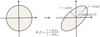Fig. 1 Geometric interpretation of q.c. mappings (figure from Lui et al. 2013a).

4 Modeling with quasi-conformal mappings

4.1 Reduction to elliptic PDEs

The Beltrami equation, Eq. (33), can be reduced to two elliptic PDEs for the real and imaginary part of f with coefficients determined by the Beltrami coefficient field μ (Lui et al. 2013b). By decomposing μ and f into μ = Re(μ) + iIm(μ) ≕ ρ + iτ and f = Re(f) + iIm(f) ≕ u + iυ, the Beltrami coefficient can be written in terms of x and y derivatives of u and υ as $$\mu =\rho +\text{i}\tau =\frac{\left({\upsilon }_x-{\upsilon }_y\right)+\text{i}\left({\upsilon }_x+u_y\right)}{\left(u_x+{\upsilon }_y\right)+\text{i}\left({\upsilon }_x-u_y\right)}.$$(42)

The υ_x and υ_y can be expressed as linear combinations of u_x and u_y, $$-{\upsilon }_x={\alpha }_1{u}_x+{\alpha }_2{u}_y,$$(43) $${\upsilon }_y={\alpha }_2{u}_x+{\alpha }_3{u}_y,$$(44)

with $${\alpha }_1=\frac{{\left(\rho -1\right)}^2+{\tau }^2}{1-{\rho }^2-{\tau }^2};{\alpha }_2=\frac{2\tau }{1-{\rho }^2-{\tau }^2};{\alpha }_3=\frac{{\left(1+\rho \right)}^2+{\tau }^2}{1-{\rho }^2-{\tau }^2}.$$(45)

On the other hand, $$u_y={\alpha }_1{\upsilon }_x+{\alpha }_2{\upsilon }_y,$$(46) $$-u_x={\alpha }_2{\upsilon }_x+{\alpha }_3{\upsilon }_y.$$(47)

Due to the symmetry of the second derivatives, it holds that $$\begin{array}{ccc}\nabla \cdot \left(\begin{array}{c}-{\upsilon }_y\\ {\upsilon }_x\end{array}\right)=0& \text{and}& \nabla \cdot \left(\begin{array}{c}{u}_y\\ -u_x\end{array}\right)=0.\end{array}$$(48)

By substituting Eqs. (43) and (44) into Eq. (48), we obtain two elliptic PDEs for u and υ, $$\nabla \cdot \left(A\left(\begin{array}{c}{u}_x\\ u_y\end{array}\right)\right)=0\text{\hspace{0.17em}and\hspace{0.17em}}\nabla \cdot \left(A\left(\begin{array}{c}{\upsilon }_x\\ {\upsilon }_y\end{array}\right)\right)=0,$$(49)

where the symmetric, positive definite matrix, A, is given by $$A=\left(\begin{array}{cc}{\alpha }_1& {\alpha }_2\\ {\alpha }_2& {\alpha }_3\end{array}\right).$$(50)

The eigenvalues λ₁ and λ₂ of A, $${\lambda }_1={\left(1-\left|\mu \right|\right)}^2,$$(51) $${\lambda }_2={\left(1+\left|\mu \right|\right)}^2,$$(52)

are strictly greater than 0 since |μ| ≤ k < 1. Since a_ij, α₁, α₂, and α₃ do not explicitly depend on x or y, Eq. (49) can be written out as $$-\text{div}\left(A\nabla u\right)=-{\displaystyle \sum _{i=1}^2{\partial }_i{\left(A\nabla u\right)}_i=-{\displaystyle \sum _{i,k=1}^2{a}_{ik}{\partial }_{ik}u.}}$$(53)

With that, we can define the two linear elliptic differential operators: $$Lu:=-{\displaystyle \sum _{i,k=1}^2{a}_{ik}{\partial }_{i,k}u,}$$(54) $$L\upsilon :=-{\displaystyle \sum _{i,k=1}^2{a}_{ik}{\partial }_{i,k}\upsilon .}$$(55)

The analytical characteristics of the two differential operators are governed by the properties of ɡ, such as adherence to the maximum principle. Similarly, the regularity of ɡ plays a critical role in determining the regularity of the associated lens mapping, particularly with respect to interior regularity. However, this work focuses on solving Lu = 0 and Lυ = 0 numerically with appropriate boundary conditions.

4.2 QCLens algorithm

The implementation of the QCLens algorithm utilizes the HiFlow3 software (Heuveline 2010), a C++-based multipurpose finite element solver. This approach discretizes the problem by employing a triangulation of the domain, Ω, with the mesh width, h. The Beltrami coefficient, –ɡ, is used to calculate the matrices, A, at each node. These matrices are integrated over the mesh using a two-dimensional quadrature formula to form the stiffness matrix and right-hand side vector. To solve the resulting elliptic PDEs for both the real and the imaginary parts of the lens mapping, finite element methods are employed. Specifically, piecewise linear functions are used to represent the solution in a finite-dimensional subspace. The solution is computed iteratively using a conjugate gradient solver, with Dirichlet or Neumann boundary conditions based on physical assumptions about the deflection field at the boundary ∂Ω.

In the spirit of reproducible research, the QCLens algorithm is publicly available on GitHub¹, including the material needed to reproduce the simulated experiments.

4.3 Extension to the sphere

Inversion methods for large areas of the sky, where the plane sky approximation can no longer be assumed, have become highly relevant with Stage IV surveys like Euclid (Euclid Collaboration: Mellier et al. 2025). Extending mass-mapping techniques to the sphere is a fundamental necessity for such surveys. A traditional approach is to decompose the sphere into overlapping patches, assume a flat approximation on each patch, reconstruct each patch independently, and recombine all patches on the sphere. It is natural to ask whether our results of the plane case can be generalized to the curved-sky treatment: If the plane sky approximation is considered as a coordinate chart around a given point on the curved surface, the Beltrami equation holds locally in this chart. However, the flat sky approximation does not provide isothermal coordinate charts, i.e., charts where the Riemannian metric is conformal to the Euclidean metric. To what extent the lens mapping can still be described in this setting as a q.c. mapping between curved surfaces will be the subject of future work.

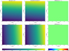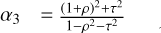
Fig. 2 Schwarzschild lens: Comparison between actual lens mapping, f = u + iυ, and calculated lens mapping, f7 = u7 + iυ7, with QCLens for a resolution of n = 7 and Dirichlet boundary conditions.

5 Experimental results

5.1 Schwarzschild lens

For the Schwarzschild lens, we obtain for the lens mapping $$\begin{array}{l}f\left(z\right)=z-\frac{1}{z}=x\left(1-\frac{1}{x^2+y^2}\right)+iy\left(1-\frac{1}{x^2+y^2}\right)\\ =:u\left(x,y\right)+i\upsilon \left(x,y\right),\end{array}$$(56)

and for the Beltrami coefficient $$\mu \left(z\right)=\frac{1}{{\overline{z}}^2}=\frac{x^2-y^2}{{\left(x^2+y^2\right)}^2}+\text{i}\frac{2xy}{{\left(x^2+y^2\right)}^2}=:\rho \left(x,y\right)+\text{i}\tau \left(x,y\right).$$(57)

For both the real and imaginary part of f, we assumed Dirichlet boundary conditions. We computed uⁿ and υⁿ using the QCLens algorithm for different resolutions n from n = 3 to n = 8 (i.e., 2ⁿ calls per coordinate direction). As shown in Fig. 2, for n = 7 we obtain an almost complete agreement between the actual and calculated lens mapping.

Here, the coordinate system was chosen such that the point (0, 0) coincides with the position of the point mass in the lens plane. Additionally, the field of view, Ω, is assumed to be the square {z = x + iy | 2 ≤ x, y ≤ 3}, such that we are in the weak lensing regime and do not cross any critical curve. As shown in Fig. 3, the deviation between the real and the calculated lens mapping can also be quantified by plotting the L₂ and H₁ error against the refinement order, n, where $$e_{L_2,w}^n={\Vert w-w^n\Vert }_{L_2}={\left({\displaystyle {\int }_{\Omega }{\left(w\left(z\right)-w^n\left(z\right)\right)}^2\text{d}z}\right)}^{\frac{1}{2}},$$(58) $$e_{H_1,w}^n={\Vert \nabla \left(w-w^n\right)\Vert }_{L_2}={\left({\displaystyle {\int }_{\Omega }{\left|\nabla w\left(z\right)-\nabla w^n\left(z\right)\right|}^2\text{d}z}\right)}^{\frac{1}{2}},$$(59)

with w ∈ {u, υ}. The errors $e_{L_2,w}^n$ and $e_{H_1,w}^n$ are the same for u and υ. As can be seen in Fig. 3, the error $e_{L_2,w}^n$ decreases quadrati-cally with increasing refinement order, n, while the error $e_{H_1,w}^n$ decreases linearly with n.

Fig. 3 Schwarzschild lens error: L2 and H1 errors for different refinement orders with Dirichlet boundary conditions. The orange and red lines overlap, as do the green and blue lines.

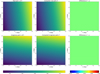Fig. 4 Singular isothermal lens: Comparison between actual lens mapping, f = u + iυ, and calculated lens mapping, f7 = u7 + iυ7, with QCLens for a resolution of n = 7 and Dirichlet boundary conditions.

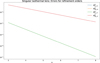Fig. 5 Singular isothermal lens error: L2 and H1 errors for different refinement orders with Dirichlet boundary conditions. The orange and red lines overlap, as do the green and blue lines.

5.2 Singular isothermal lens

For the singular isothermal lens, we obtain for the lens mapping $$\begin{array}{l}f\left(z\right)=z-\frac{z}{\left|\overline{z}\right|}=x\left(1-\frac{1}{\sqrt{x^2+y^2}}\right)+\text{i}y\left(1-\frac{1}{\sqrt{x^2+y^2}}\right)\\ =:u\left(x,y\right)+\text{i}\upsilon \left(x,y\right),\end{array}$$(60)

and for the Beltrami coefficient $$\begin{array}{l}\mu \left(z\right)=\frac{z^2}{2{\left|\overline{z}\right|}^3-{\left|\overline{z}\right|}^2}=\frac{\left(x^2-y^2\right)}{2{\left(x^2+y^2\right)}^{\frac{3}{2}}-\left(x^2+y^2\right)}+\text{i}\frac{2xy}{2{\left(x^2+y^2\right)}^{\frac{3}{2}}-\left(x^2+y^2\right)}\\ =:\rho \left(x,y\right)+\text{i}\tau \left(x,y\right).\end{array}$$(61)

Using the same coordinate system and field of view as for the Schwarzschild lens, we obtain analogous results under the assumption of Dirichlet boundary conditions. As in the Schwarzschild lens experiment, the lens mapping computed for n = 7 shows near-perfect agreement with the actual mapping, as illustrated in Fig. 4. Correspondingly, Fig. 5 demonstrates that the error $e_{L_2,w}^n$ decreases quadratically with increasing refinement order n, while the error $e_{H_1,w}^n$ exhibits a linear decrease.

6 Conclusion

We have proposed a novel inversion algorithm for weak gravitational lensing based on the q.c. mapping framework. By reformulating the lens equation as a Beltrami equation, the problem was reduced to solving elliptic PDEs for the real and the imaginary part of the lens mapping. The QCLens algorithm was applied to analytically solvable cases, such as the Schwarzschild and singular isothermal lens models, demonstrating consistency with expected results. Additionally, we have discussed the feasibility of extending the approach to spherical geometries, which will be necessary for future surveys like Euclid. These findings provide a foundation for further exploration of mass-mapping techniques within this framework.

Acknowledgements

We thank Prof. Björn Malte Schäfer for his early discussions on the subject and for valuable comments on earlier versions of the manuscript.

References

All Figures

	Fig. 1 Geometric interpretation of q.c. mappings (figure from Lui et al. 2013a).
In the text

	Fig. 2 Schwarzschild lens: Comparison between actual lens mapping, f = u + iυ, and calculated lens mapping, f7 = u7 + iυ7, with QCLens for a resolution of n = 7 and Dirichlet boundary conditions.
In the text

	Fig. 3 Schwarzschild lens error: L2 and H1 errors for different refinement orders with Dirichlet boundary conditions. The orange and red lines overlap, as do the green and blue lines.
In the text

	Fig. 4 Singular isothermal lens: Comparison between actual lens mapping, f = u + iυ, and calculated lens mapping, f7 = u7 + iυ7, with QCLens for a resolution of n = 7 and Dirichlet boundary conditions.
In the text

	Fig. 5 Singular isothermal lens error: L2 and H1 errors for different refinement orders with Dirichlet boundary conditions. The orange and red lines overlap, as do the green and blue lines.
In the text

References

- Bartelmann, M., & Schneider, P. 2001, Phys. Rep., 340, 291 [Google Scholar]
- Brough, S., Collins, C., Demarco, R., et al. 2020, arXiv e-prints [arXiv: 2001.11067] [Google Scholar]
- Euclid Collaboration (Mellier, Y., et al.) 2025, A&A, 697, Al [Google Scholar]
- Forster, Ο. 2012, Lectures on Riemann Surfaces (Berlin: Springer Science & Business Media) [Google Scholar]
- Heuveline, V. 2010, ACM Trans. Math. Softw., 37, 1 [CrossRef] [Google Scholar]
- Kaiser, N., & Squires, G. 1993, ApJ, 404, 441 [Google Scholar]
- Kilbinger, M. 2015, Rep. Prog. Phys., 78, 086901 [Google Scholar]
- Lui, L. M., Gu, X., & Yau, S.-T. 2013a, arXiv e-prints [arXiv: 1307.2679] [Google Scholar]
- Lui, L. M., Lam, K. C., Wong, T. W., & Gu, X. 2013b, SIAM J. Imaging Sei., 6, 1880 [Google Scholar]
- Meneghetti, M. 2021, Introduction to Gravitational Lensing - With Python Examples (Berlin: Springer Nature) [Google Scholar]
- Seitz, C., & Schneider, P. 1997, A&A, 318, 687 [NASA ADS] [Google Scholar]
- Spergel, D., Gehreis, N., Baltay C., et al. 2015, Wide-Field InfrarRed Survey Telescope-Astrophysics Focused Telescope Assets WFIRST-AFTA 2015 Report [Google Scholar]
- Starck, J.-L., Themelis, K. E., Jeffrey, N., Peel, Α., & Lanusse, F. 2021, A&A, 649, A30 [NASA ADS] [CrossRef] [EDP Sciences] [Google Scholar]
- Straumann, N. 1997, arXiv e-prints [arXiv:astro-ph/9703103vl] [Google Scholar]
- Umetsu, K. 2020, Astron. Astrophys. Rev, 28, 7 [Google Scholar]