© The Authors 2025

1. Introduction

Magnetohydrodynamic (MHD) waves are heavily affected when propagating in a medium with nonuniform properties, such as the solar atmosphere. One direct consequence of nonuniformity is the coupling between the various MHD wave modes (see, e.g., Cally & Bogdan 2024). Owing to the coupling, the perturbations associated with MHD waves generally display mixed properties of the pure modes depending on position and/or time (see, e.g., Soler & Goossens 2024). However, it has been shown that the distinct pure modes remain definable (see, e.g., Raboonik et al. 2024). As the plasmas in the lower atmosphere and solar prominences are in a state of partial ionization, effects caused by ion-neutral collisions, such as ambipolar diffusion, can also affect wave propagation and coupling in such plasmas (Soler 2024).

In the vertically stratified lower solar atmosphere, the profiles of sound and Alfvén speeds converge at the so-called equipartition layer. This convergence facilitates coupling between the distinct magnetosonic modes. In addition, in the presence of inclined magnetic fields, conversion to Alfvén waves is also possible. Theoretical studies have extensively explored this process, which may be of particular importance above sunspots (see, e.g., Cally 2001; Khomenko & Collados 2015; Cally & Bogdan 2024). In this context, Cally & Khomenko (2018) examined the conversion from fast to Alfvén modes in the presence of ambipolar diffusion, while Popescu Braileanu & Keppens (2021) explored the conversion from fast to slow magnetosonic modes under similar conditions. Notably, their results suggest that the fundamental characteristics of the mode conversion process remain largely unchanged compared to the ideal case. However, the primary difference is the damping caused by ambipolar diffusion. A detailed analysis of magnetosonic mode conversion within the two-fluid framework was presented in Cally & Gómez-Míguez (2023). They derived a transformation coefficient that includes a correction term owing to ion-neutral collisions, although it was found to be of small importance under solar atmospheric conditions. On the other hand, Cally & Khomenko (2019) and Khomenko & Cally (2019) studied the fast-to-Alfvén mode conversion in an assembly of small-scale flux tubes. They found that the impact of ambipolar diffusion was amplified by the presence of the flux tube structure.

Another nonideal mechanism that can be of potential relevance for wave coupling in the solar plasma is the Hall effect. In the presence of partial ionization, this effect is enhanced by the collisions with neutrals (Pandey & Wardle 2008). Conversion from fast to Alfvén modes mediated by the Hall term was studied in Cally & Khomenko (2015) and González-Morales et al. (2019), whereas the coupling between slow and Alfvén modes was analyzed in Raboonik & Cally (2019). While the Hall-mediated conversion from fast to Alfvén modes requires significantly high frequencies to be efficient, the conversion from slow to Alfvén modes can be relevant at much lower frequencies. The results of these studies are applicable in the photosphere and lower chromosphere.

Resonant absorption can be considered as another type of mode conversion process (see, e.g., Goossens et al. 2011). It describes how MHD wave energy is absorbed into the continuous Alfvén or slow spectra. This process depends on gradients across the magnetic field direction. The resonant absorption of Alfvénic waves in partially ionized magnetic flux tubes, such as prominence threads or chromospheric spicules, was studied by Soler et al. (2009) using the single-fluid model and by Soler et al. (2012) in the two-fluid framework. The latter study analyzed the decoupling of ions and neutrals within the extremely thin collisional layer around the resonance. This decoupling causes dissipation and large velocity gradients that may lead to substantial plasma heating within the narrow layer.

Observations often show that MHD waves and flows are simultaneously present in the solar atmosphere (e.g., Okamoto et al. 2007; Ofman & Wang 2008; De Pontieu & McIntosh 2010; Tian et al. 2012; Ofman & Kucera 2020). This gives rise to another potential wave coupling mechanism driven by the flows. A shear flow entails a spatial inhomogeneity, and it has been shown that this causes linear coupling and mutual transformation between the MHD waves (see, e.g., Chagelishvili et al. 1996a, 1997; Rogava & Mahajan 1997; Gogoberidze et al. 2004, among others). A velocity shear causes significant change in the very nature of the eigenvalue problem associated with linear waves. The corresponding eigenvalue problem becomes non-self-adjoint, leading to non-orthogonal eigenfunctions with no independent temporal evolution. Consequently the exponential temporal dependence of the asymptotic normal mode analysis cannot completely describe the evolution of the coupled waves. Another approach is needed to understand the wave conversion and the energy exchange between modes. The so-called nonmodal analysis (see, e.g., Schmid 2007; Camporeale 2012) has been used in previous studies dealing with shear-induced wave transformations in a wide variety of astrophysical and geophysical contexts (see, e.g., Chagelishvili et al. 1994, 1996b, 1997; Rogava & Mahajan 1997; Rogava et al. 1998, 1999). Although there are some works that have studied nonmodal effects on MHD waves in the solar atmosphere and the solar wind (see Poedts et al. 1998, 1999), no previous work has analyzed the shear-induced wave coupling in partially ionized solar plasmas and the role of ambipolar diffusion in the process.

We aim to investigate the wave coupling and energy transfer mechanism driven by shear flows in regions of the solar atmosphere where the plasma is partially ionized, as the role of ambipolar diffusion can be important in these places. In this initial paper, we include the derivation of the general governing equations and specifically apply them to explore the mutual transformation between the fast magnetosonic wave and the Alfvén wave in the pressureless approximation. Later, in a related forthcoming paper, the investigation will be extended by considering the role of gas pressure, and thus the coupling with the slow magnetosonic wave will be studied.

2. Background and method

In order to study the essential features of the shear-induced mode coupling, we consider a simple background composed of a uniform partially ionized plasma with a constant magnetic field. We use a Cartesian coordinate system so that the background magnetic field is along the z-direction, namely ${\mathit{B}}_0=B_0\widehat{z}$, with B₀ constant. The thermal pressure is also uniform. There is a shear flow parallel to the direction of the magnetic field and whose velocity varies in the x-direction, i.e., across the magnetic field. We use a linear variation for the background flow velocity as ${\mathit{V}}_0=Ax\widehat{z}$, with the constant A measuring the strength of the shear. This configuration, although simple, contains the basic ingredients for our study. This is due to fact that, for small perturbations with wavelengths much shorter than the length scale of the flow variation, any arbitrary flow can locally be approximated by a linear flow. Essentially, this is the same setup as that used in Poedts et al. (1998), with the difference that we allow the plasma to be partially ionized. The role of partial ionization is here included by considering the nonideal mechanism of ambipolar diffusion.

2.1. Main equations

We considered the single-fluid MHD equations that include ambipolar diffusion to account for ion-neutral collision effects in a partially ionized plasma (see, e.g., Khomenko et al. 2014; Ballester et al. 2018), namely,

$$\begin{array}{cc}\hfill \frac{D\rho }{\mathit{Dt}}& =-\rho \mathrm{\nabla }·\mathit{v},\hfill \end{array}$$(1a)

$$\begin{array}{cc}\hfill \rho \frac{D\mathit{v}}{\mathit{Dt}}& =-\mathrm{\nabla }p+\mathit{J}\times \mathit{B}\hfill \end{array}$$(1b)

$$\begin{array}{cc}\hfill \frac{\partial \mathit{B}}{\partial t}& =\mathrm{\nabla }\times (\mathit{v}\times \mathit{B})+\mathrm{\nabla }\times \left\{\frac{{\mu }_0{\eta }_A}{{|\mathit{B}|}^2}[(\mathit{J}\times \mathit{B})\times \mathit{B}]\right\},\hfill \end{array}$$(1c)

$$\begin{array}{cc}\hfill \frac{\mathit{Dp}}{\mathit{Dt}}& =\frac{\gamma p}{\rho }\frac{D\rho }{\mathit{Dt}}+(\gamma -1){\mu }_0{\eta }_A{|\frac{\mathit{B}}{|\mathit{B}|}\times [\mathit{J}\times \frac{\mathit{B}}{|\mathit{B}|}]|}^2,\hfill \end{array}$$(1d)

$$\begin{array}{cc}\hfill p& =\rho \mathcal{R}\frac{T}{\stackrel{\sim }{\mu }},\hfill \end{array}$$(1e)

where $\frac{D}{\mathit{Dt}}=\frac{\partial }{\partial t}+\mathit{v}·\mathrm{\nabla }$ is the total derivative. The equations in System (1) are the continuity equation, momentum equation, induction equation, energy equation, and ideal gas equation, respectively. In these expressions, v is the velocity, B is the magnetic field, ρ is the mass density, p is the thermal pressure, and J = (∇×B)/μ₀ is the current density; with μ₀ as the magnetic permeability, η_A is the coefficient of ambipolar diffusion, γ is the adiabatic index, T is the temperature, ℛ is the ideal gas constant, and $\stackrel{\sim }{\mu }$ is the mean atomic weight. As our focus shall be put on the effects of ambipolar diffusion, other nonideal mechanisms, such as viscosity, radiative losses, thermal conduction, or the Hall effect are neglected. The ambipolar diffusion is in many cases the most important nonideal effect in partially ionized solar plasmas, although the Hall effect can be of importance in certain processes, such as reconnection or magneto-convection (see, e.g., Pandey & Wardle 2008; Threlfall et al. 2012; González-Morales et al. 2020). In the middle and high chromosphere, as well as in solar prominences, the ambipolar diffusion is expected to be the dominant effect (see details in, e.g., Khomenko & Collados 2012; Ballester et al. 2018). Gravity is also dropped.

We use the small perturbation theory to obtain a set of equations that describe the interplay between the MHD waves and the background shear flow. We assumed that all the physical variables can be written as

$$\begin{array}{c}\hfill f(\mathit{r},t)=f_0(\mathit{r})+f_1(\mathit{r},t),\end{array}$$(2)

where f₀ is the equilibrium value and f₁ is a perturbation, which contains the temporal dependence and is assumed to be much smaller than the equilibrium value, i.e., |f₀|≫|f₁|. Hence, we linearized System (1), and the resulting linearized equations are

$$\begin{array}{cc}\hfill ({\partial }_t+Ax{\partial }_z)d& =-({\partial }_x{v}_x+{\partial }_y{v}_y+{\partial }_z{v}_z),\hfill \end{array}$$(3a)

$$\begin{array}{cc}\hfill ({\partial }_t+Ax{\partial }_z)v_x& =-V_s^2{\partial }_{x}d+V_A^2({\partial }_z{b}_x-{\partial }_x{b}_z),\hfill \end{array}$$(3b)

$$\begin{array}{cc}\hfill ({\partial }_t+Ax{\partial }_z)v_y& =-V_s^2{\partial }_{y}d+V_A^2({\partial }_z{b}_y-{\partial }_y{b}_z),\hfill \end{array}$$(3c)

$$\begin{array}{cc}\hfill ({\partial }_t+Ax{\partial }_z)v_z& =-V_s^2{\partial }_{z}d-A{v}_x,\hfill \end{array}$$(3d)

$$\begin{array}{cc}\hfill ({\partial }_t+Ax{\partial }_z)b_x& ={\partial }_z{v}_x+{\eta }_A({\partial }_z^2{b}_x-{\partial }_{\mathit{zx}}^2{b}_z),\hfill \end{array}$$(3e)

$$\begin{array}{cc}\hfill ({\partial }_t+Ax{\partial }_z)b_y& ={\partial }_z{v}_y+{\eta }_A({\partial }_z^2{b}_y-{\partial }_{\mathit{zy}}^2{b}_z),\hfill \end{array}$$(3f)

where we introduced the dimensionless perturbations of density, d = ρ₁/ρ₀, and magnetic field, b_i = B_1i/B₀, with i = x, y, z. To simplify the notation, we dropped the subscript 1 from the components of the velocity perturbation so that we simply write v_i, with i = x, y, z. We note that the z-component of the linearized induction equation is not used and is conveniently replaced by the solenoidal constraint, namely

$$\begin{array}{c}\hfill {\partial }_x{b}_x+{\partial }_y{b}_y+{\partial }_z{b}_z=0.\end{array}$$(4)

Additionally, V_A and V_s represent the equilibrium Alfvén and sound speeds, respectively, and are defined by

$$\begin{array}{c}\hfill V_A=\sqrt{\frac{B_0^2}{\mu {\rho }_0}},V_s=\sqrt{\frac{\gamma p_0}{{\rho }_0}}·\end{array}$$(5)

It should be noted that the source term due to ambipolar heating in Equation (1d) drops as a result of the linearization, since it is a second-order term in the perturbations. Consequently, the internal energy equation becomes adiabatic in the linear approximation.

2.2. Nonmodal analysis

The usual asymptotic normal mode analysis is not suited to studying the interaction between MHD waves and shear flows since the associated eigenvalue problem becomes non-self-adjoint due to the background flow inhomogeneity (Trefethen et al. 1993; Chagelishvili et al. 1993). This has led to the use of so-called nonmodal approach (Mahajan & Rogava 1999; Bodo et al. 2001; Camporeale 2012), in which one considers the temporal evolution of the spatial Fourier harmonics of the perturbations, but without any spectral expansion in time.

Following the standard method of the nonmodal approach, we introduced a change of variables,

$$\begin{array}{c}\hfill x\prime =x,y\prime =y,z\prime =z-Axt,t\prime =t,\end{array}$$(6)

in order to transform the spatial inhomogeneity into a temporal one. In the following expressions, the prime symbol ′ on the new variables is dropped for simplicity. We continued by taking the spatial Fourier transform of the perturbations. Hence, any perturbation, generally represented as F, is expressed as

$$\begin{array}{c}\hfill F(x,y,z,t)={\displaystyle \int \stackrel{\sim }{F}}(k_x,k_y,k_z,t)e^{i(k_{x}x+k_{y}y+k_{z}z)}d{k}_{x}d{k}_{y}d{k}_z,\end{array}$$(7)

where $\stackrel{\sim }{F}$ is the Fourier transform of F, with k_x, k_y, and k_z the wave numbers in the x, y, and z directions, respectively. This allows us to rewrite the set of equations in System (3) in terms of the Fourier transforms of the perturbations, where all spatial derivatives are replaced by products with the respective wave numbers. Introducing dimensionless variables, the new set of equations in Fourier space is

$$\begin{array}{cc}\hfill D^{(1)}& =K_x{u}_x+K_y{u}_y+u_z,\hfill \end{array}$$(8a)

$$\begin{array}{cc}\hfill u_x^{(1)}& =-{\epsilon }^2{K}_{x}D+(1+K_x^2)b_x+K_x{K}_y{b}_y,\hfill \end{array}$$(8b)

$$\begin{array}{cc}\hfill u_y^{(1)}& =-{\epsilon }^2{K}_{y}D+K_x{K}_y{b}_x+(1+K_y^2)b_y,\hfill \end{array}$$(8c)

$$\begin{array}{cc}\hfill u_z^{(1)}& =-{\epsilon }^{2}D-R{u}_x,\hfill \end{array}$$(8d)

$$\begin{array}{cc}\hfill b_x^{(1)}& =-u_x-{\stackrel{\sim }{\eta }}_A(1+K_x^2)b_x-{\stackrel{\sim }{\eta }}_A{K}_x{K}_y{b}_y,\hfill \end{array}$$(8e)

$$\begin{array}{cc}\hfill b_y^{(1)}& =-u_y-{\stackrel{\sim }{\eta }}_A{K}_x{K}_y{b}_x-{\stackrel{\sim }{\eta }}_A(1+K_y^2)b_y,\hfill \end{array}$$(8f)

where f⁽ⁿ⁾ denotes the nth-order temporal derivative of f, and we used Equation (4) to eliminate b_z. The dimensionless variables and coefficients are defined as

$$\begin{array}{cc}\hfill D& =i\stackrel{\sim }{d},b_x=i{\stackrel{\sim }{b}}_x,b_y=i{\stackrel{\sim }{b}}_y,\hfill \end{array}$$(9a)

$$\begin{array}{cc}\hfill u_x& =\frac{{\stackrel{\sim }{v}}_x}{V_A},u_y=\frac{{\stackrel{\sim }{v}}_y}{V_A},u_z=\frac{{\stackrel{\sim }{v}}_z}{V_A},\hfill \end{array}$$(9b)

$$\begin{array}{cc}\hfill K_x& =\frac{k_x}{k_z}-R\tau =K_{x0}-R\tau ,K_y=\frac{k_y}{k_z},\hfill \end{array}$$(9c)

$$\begin{array}{cc}\hfill R& =\frac{A}{V_A{k}_z},\epsilon =\frac{V_s}{V_A},{\stackrel{\sim }{\eta }}_A=\frac{k_z{\eta }_A}{V_A}·\hfill \end{array}$$(9d)

We note that the velocities are all normalized to the Alfvén speed. The new temporal variable, τ, is normalized to the Alfvén time, so that τ = V_Ak_zt. In addition, R measures the normalized strength of the velocity shear and ε represents, essentially, the plasma β, i.e., the importance of the thermal pressure with respect to the magnetic pressure. Importantly, we note that in this formalism K_x is a function of time. If K_x0 > 0 and for a sufficiently long time, K_x will change sign. This can be understood as a reflection of the wave caused by the shear flow.

The set of Equations (8) may further be reduced into a system of three intercoupled second-order ordinary differential equations (ODEs) by introducing the new variable ψ = D + K_xb_x + K_yb_y and expressing u_x, u_y and u_z and their temporal derivatives in terms of the magnetic field perturbations, namely

$$\begin{array}{cc}\hfill {\psi }^{(2)}+{\omega }_1^2\psi & =(C_{12}+{\gamma }_1)b_x+(C_{13}+{\gamma }_2)b_y\hfill \\ \hfill & +J_1{b}_x^{(1)}+J_2{b}_y^{(1)},\hfill \end{array}$$(10a)

$$\begin{array}{cc}\hfill b_x^{(2)}+({\omega }_2^2+{\gamma }_3)b_x& =C_{12}\psi +(C_{23}+{\gamma }_4)b_y\hfill \\ \hfill & +J_3{b}_x^{(1)}+J_4{b}_y^{(1)},\hfill \end{array}$$(10b)

$$\begin{array}{cc}\hfill b_y^{(2)}+{\omega }_3^2{b}_y& =C_{13}\psi +(C_{23}+{\gamma }_4)b_x\hfill \\ \hfill & +J_4{b}_x^{(1)}+J_5{b}_y^{(1)},\hfill \end{array}$$(10c)

where the following auxiliary notation has been introduced: the uncoupled oscillation eigenfrequencies, ω₁, ω₂, and ω₃, namely

$$\begin{array}{cc}\hfill {\omega }_1& =\epsilon ,\hfill \end{array}$$(11a)

$$\begin{array}{cc}\hfill {\omega }_2& =\sqrt{1+(1+{\epsilon }^2)K_x^2},\hfill \end{array}$$(11b)

$$\begin{array}{cc}\hfill {\omega }_3& =\sqrt{1+(1+{\epsilon }^2)K_y^2};\hfill \end{array}$$(11c)

the ideal coupling coefficients, C_ij, namely

$$\begin{array}{c}\hfill C_{12}={\epsilon }^2{K}_x,C_{13}={\epsilon }^2{K}_y,C_{23}=-(1+{\epsilon }^2)K_x{K}_y;\end{array}$$(12)

and the nonideal coefficients, γ_i and J_i, which are associated with coupling and dissipation due to ambipolar diffusion, namely

$$\begin{array}{cccc}\hfill {\gamma }_1& ={\stackrel{\sim }{\eta }}_{A}R(2+4K_x^2+K_y^2),\hfill & \hfill {\gamma }_2& =3{\stackrel{\sim }{\eta }}_{A}R{K}_x{K}_y,\hfill \end{array}$$(13a)

$$\begin{array}{cccc}\hfill {\gamma }_3& =-2{\stackrel{\sim }{\eta }}_{A}R{K}_x,\hfill & \hfill {\gamma }_4& ={\stackrel{\sim }{\eta }}_{A}R{K}_y,\hfill \end{array}$$(13b)

$$\begin{array}{cccc}\hfill J_1& =-K_x{\stackrel{\sim }{\eta }}_A(1+K_x^2+K_y^2),\hfill & \hfill J_4& =-{\stackrel{\sim }{\eta }}_A{K}_x{K}_y,\hfill \end{array}$$(13c)

$$\begin{array}{cccc}\hfill J_2& =-K_y{\stackrel{\sim }{\eta }}_A(1+K_x^2+K_y^2),\hfill & \hfill J_5& =-{\stackrel{\sim }{\eta }}_A(1+K_y^2),\hfill \end{array}$$(13d)

$$\begin{array}{cc}\hfill J_3& =-{\stackrel{\sim }{\eta }}_A(1+K_x^2).\hfill \end{array}$$(13e)

The process to arrive at the set of Equations (10) is summarized as follows. To obtain Equations (10b) and (10c), we begin by differentiating Equations (8e) and (8f) with respect of time and then substituting the expressions for u_x⁽¹⁾ and u_y⁽¹⁾ into Equations (8b) and (8c), respectively. Subsequently, we replace D by the new variable ψ. To arrive at Equation (10a), we start by substituting u_x and u_y from Equations (8e) and (8f) into Equation (8a). The resulting expression is then differentiated with respect of time and u_z⁽¹⁾ is eliminated using Equation (8d). Later, u_x is again substituted using Equation (8e). Finally, we again replace D by the new variable ψ.

System (10) describes coupled linear oscillations with three degrees of freedom in a plasma with ambipolar diffusion and a shear flow. Owing to presence of shear in the flow, i.e., when R ≠ 0, some of the coefficients have time-dependent behavior. This set of equations is quite general and describes all the linear MHD modes, their mutual transformations and interaction with the shear flow, and the damping owing to ambipolar diffusion. Generally, the linear MHD modes are the Alfvén wave, AW, the fast magnetosonic wave, FMW, and the slow magnetosonic wave, SMW.

To compare with the previous results published in Poedts et al. (1998) corresponding to the case without diffusion, we set ${\stackrel{\sim }{\eta }}_A=0$ and System (10) simplifies to

$$\begin{array}{cc}\hfill {\psi }^{(2)}+{\omega }_1^2\psi & =C_{12}{b}_x+C_{13}{b}_y,\hfill \end{array}$$(14a)

$$\begin{array}{cc}\hfill b_x^{(2)}+{\omega }_2^2{b}_x& =C_{12}\psi +C_{23}{b}_y,\hfill \end{array}$$(14b)

$$\begin{array}{cc}\hfill b_y^{(2)}+{\omega }_3^2{b}_y& =C_{13}\psi +C_{23}{b}_x.\hfill \end{array}$$(14c)

This set of three equations consistently reverts to that given in Poedts et al. (1998).

The Wolfram Mathematica environment has been used to obtain numerical solutions of System (10) for prescribed initial conditions and a given set of model parameters. We used the module NDSolve to perform the integration and chose a small enough time step to avoid introducing relevant errors. This has been determined by convergence tests. The numerical solution is stored as an InterpolatingFunction for each perturbation, which allows for their manipulation and representation as if they were analytical functions.

2.3. Considerations about wave coupling

Before exploring the numerical solutions of the system of Equations (10), here we enumerate some considerations that can be useful to understand the results. These are based on previous findings discussed in, e.g., Chagelishvili et al. (1996a, 1997), Poedts et al. (1998), Gogoberidze et al. (2004), among others.

We begin by studying how the coupling of the MHD modes can occur in the case where only two modes are considered without dissipation (Morse 1981). In this situation, we can describe the system mathematically as a pair of coupled linear oscillators, which leads to the following set of second-order ODEs for the variables F₁ and F₂:

$$\begin{array}{c}\hfill F_1^{(2)}+{\omega }_1^2{F}_1+C{F}_2=0,F_2^{(2)}+{\omega }_2^2{F}_2+C{F}_1=0,\end{array}$$(15)

where ω₁ and ω₂ are the oscillator eigenfrequencies and C is the coupling coefficient. If one allows both oscillators to move simultaneously, it will usually result in a nonperiodic motion (Morse 1981). However, if the eigenfrequencies and coupling coefficient are constant, the general solution of the system can always be described as a combination of the normal modes. The normal frequencies of the coupled oscillations, Ω_±, can be determined with

$$\begin{array}{c}\hfill {\mathrm{\Omega }}_{\pm }^2=\frac{1}{2}[({\omega }_1^2+{\omega }_2^2)\pm \sqrt{({\omega }_1^2-{\omega }_2^2)+4C^2}].\end{array}$$(16)

We note that the value of Ω₋ is smaller than either ω₁ or ω₂, while Ω₊ is larger than both eigenfrequencies, meaning that the coupling will always spread apart the natural frequencies.

As one can see in the eigenfrequencies and coupling coefficients of our system, in Equations (11) and (12), they depend on time through K_x, thus making the canonical theory of coupled oscillation invalid. However, when R ≪ 1, the system evolves slowly enough, and the standard theory of coupled oscillations may be a useful reference in the interpretation of the actual coupling. In the case where the three MHD waves are considered, we can use the eigenfrequencies of the ideal waves as a reference. In our normalized notation these frequencies are

$$\begin{array}{cc}\hfill {\mathrm{\Omega }}_{F,S}^2& =\frac{1}{2}{K}^2(1+{\epsilon }^2)(1\pm \sqrt{1-\frac{4{\epsilon }^2}{K^2{(1+{\epsilon }^2)}^2}}),\hfill \end{array}$$(17a)

$$\begin{array}{cc}\hfill {\mathrm{\Omega }}_A& =1,\hfill \end{array}$$(17b)

where K² = 1 + K_x² + K_y² represents the modulus of the wave vector squared and the subscripts F, S, and A correspond to the FMW, the SMW, and the AW, respectively. Strictly speaking, these frequencies are not valid in our setup due to the temporal variation of some parameters and the ambipolar diffusion. The difference between coupled and uncoupled frequencies is presumably small. This happens when the temporal variation of the wave number K_x(τ) is slow enough, which is realized when ∂_τΩ_i ≪ Ω_i², with i = F, S, A.

When the eigenfrequencies and/or coupling coefficient vary slowly in time, the system displays mutual transformation with the corresponding energy transfer between the three modes (Chagelishvili et al. 1996a, 1997; Kotkin & Serbo 2013). Similar problems have been studied in the past and two necessary conditions were found for the effectiveness of the energy exchange between weakly coupled oscillators (see Kotkin & Serbo 2013): (1) A so-called degeneration region (DR) should exist where |Ω_i² − Ω_j²|≤|C_ij(τ)|. Here Ω_i, j represents the frequencies of two oscillation modes that couple and C_ij the corresponding coupling coefficient. For the weak coupling case, this implies that Ω_i ≃ Ω_j, thus the maximum energy exchange between modes happens when their frequencies are approximately the same. (2) The DR has to be crossed slowly. In other words, the shear-modified frequencies have to vary slowly enough so that $|{\mathrm{\Omega }}_{i,j}^{(1)}(\tau )|\ll |C_{\mathit{ij}}(\tau )|$. This condition readily holds in the DR when we consider a low shear flow with R ≪ 1. Hence, from the first condition we learn that the DR has to be found in the neighborhood of the time that minimizes the difference between frequencies, so that |K_x(τ)| ≤ 1 (Poedts et al. 1998). This characteristic time where K_x(τ) = 0 is denoted as τ_* and can be calculated as

$$\begin{array}{c}\hfill {\tau }_{\ast }=\frac{K_{x0}}{R}·\end{array}$$(18)

From this expression we can see that the temporal scale of energy exchange between background flow and wave modes is of the order ∼R⁻¹. Furthermore, τ_* can also be interpreted as the time at which the effective reflection of the wave propagation in the x-direction occurs. The sheared background flow attempts to change the direction of wave propagation across the flow, resulting in the temporal dependence of K_x(τ). When τ = τ_* and for K_x0 > 0 initially, the value of K_x(τ) reaches zero and begins to increase negatively, resulting in the effective reflection of the wave. When this phenomenon of effective wave reflection happens, the shear flow could be seen from an external observer as a driver of the waves.

On the other hand, from the second condition it can be shown that the temporal scale of resonant interaction, this is the time scale of energy exchange between wave modes, is of the order ∼R^{−1 + 1/R} (see details in Gogoberidze et al. 2004). If we consider the low shear case (R ≪ 1), we reach the conclusion that the resonant interaction of waves is a faster process than the energy exchange between the shear flow and wave modes (Gogoberidze et al. 2004).

Additionally, it is important to note that the wave transformation is subject to temporal restrictions but not to spatial ones. Thus, transformation of waves in shear flows may potentially happen throughout the medium, but only at the specific times when the DR is realized locally (Chagelishvili et al. 1997).

Here, we clarify the necessary system parameter conditions to achieve the DR, so that the mutual transformation between the MHD waves can happen:

• Mutual transformation between FMW and AW:

  $$\begin{array}{c}\hfill {\mathrm{\Omega }}_F^2\simeq {\mathrm{\Omega }}_A^2,\epsilon <1,K_y\ll 1.\end{array}$$

• Mutual transformation between FMW and SMW:

  $$\begin{array}{c}\hfill {\mathrm{\Omega }}_F^2\simeq {\mathrm{\Omega }}_S^2,\epsilon \simeq 1.\end{array}$$

• Mutual transformation between AW and SMW:

  $$\begin{array}{c}\hfill {\mathrm{\Omega }}_A^2\simeq {\mathrm{\Omega }}_S^2,\epsilon >1.\end{array}$$

• Mutual transformation between the three modes:

  $$\begin{array}{c}\hfill {\mathrm{\Omega }}_F^2\simeq {\mathrm{\Omega }}_A^2\simeq {\mathrm{\Omega }}_S^2,\epsilon \simeq 1,K_y\ll 1.\end{array}$$

A particular case of the mutual transformation between the three modes is the so-called beat regime, which is realized when R ≪ K_x0 ≪ 1. This leads to an inherently efficient coupling (see Rogava & Mahajan 1997; Poedts et al. 1998).

The analysis of the energy associated to the wave modes can be useful to understand the coupling. Following the process described in Walker (2005), we derived a conservation equation for the energy of the linear perturbations, namely

$$\begin{array}{c}\hfill {\partial }_{t}U+{\mathit{V}}_0·\mathrm{\nabla }U+\mathrm{\nabla }·\mathbf{\Pi }=H_{\mathrm{flow}}+H_{\mathrm{diff}.},\end{array}$$(19)

where

$$\begin{array}{c}\hfill U=\frac{1}{2}{\rho }_0|{\mathit{v}}_1{|}^2+\frac{1}{2{\mu }_0}{|{\mathit{B}}_1|}^2+\frac{1}{2\gamma p_0}{p}_1^2\end{array}$$(20)

is the energy density, with the term V₀ ⋅ ∇U accounting for the advection of the energy density by the mass flow;

$$\begin{array}{c}\hfill \mathbf{\Pi }=(p_1+\frac{{\mathit{B}}_0·{\mathit{B}}_1}{{\mu }_0}){\mathit{v}}_1-\frac{{\mathit{v}}_1·{\mathit{B}}_1}{{\mu }_0}{\mathit{B}}_0\end{array}$$(21)

is the waves energy flux;

$$\begin{array}{c}\hfill H_{\mathrm{flow}}={\mathit{B}}_1·\left[({\mathit{B}}_1·\mathrm{\nabla }){\mathit{V}}_0\right]-{\mathit{v}}_1·\left[({\mathit{v}}_1·\mathrm{\nabla }){\mathit{V}}_0\right]\end{array}$$(22)

is a source-sink term due to the energy exchange between the waves and the shear flow, and

$$\begin{array}{c}\hfill H_{\mathrm{diff}.}=\frac{{\eta }_A}{|{\mathit{B}}_0{|}^2}{\mathit{B}}_1·\{((\mathrm{\nabla }\times {\mathit{B}}_1)\times {\mathit{B}}_0)\times {\mathit{B}}_0\},\end{array}$$(23)

is the energy dissipation term due to ambipolar diffusion. The expressions in Equations (20)–(23) are written in a general form. It is instructive to obtain the expression of H_flow in the specific configuration of our background flow with ${\mathit{V}}_0=Ax\widehat{z}$, namely

$$\begin{array}{c}\hfill H_{\mathrm{flow}}=A(B_{1x}{B}_{1z}-v_x{v}_z).\end{array}$$(24)

First, it is worth noting that H_flow can be either positive or negative, depending on the phase relations between the oscillating perturbations, so that it can act as either an energy source term (energy goes from the flow to the waves) or an energy sink term (energy goes from the waves to the flow). Equation (24) also shows that the energy exchange between waves and flow is proportional to the shear strength, A. This means that the larger the shear, the more important this energy exchange is. In addition, H_flow involves the x- and z-components of the velocity and magnetic field perturbations, but not the y-components. As a consequence of this, pure Alfvén waves, which are polarized in the y-direction, are unable the exchange energy with the flow. In relation to this comment, Chagelishvili et al. (1996b) showed that perturbations in thermal or magnetic pressure are required for the energy exchange with the flow to happen. Hence, only the waves capable of generating such perturbations can exchange energy with the flow. Consequently, as linear Alfvén waves are incompressible and do not perturb the pressure field, they cannot exchange energy with the background flow by themselves via shear-induced processes (Chagelishvili et al. 1997).

Ambipolar diffusion appears in the wave energy equation as a sink term (Equation (23)). Since energy is a conserved quantity, the energy lost by the wave due to ambipolar diffusion must be deposited into the plasma and converted into internal energy. However, as previously discussed, the internal energy equation becomes adiabatic under linearization, because the ambipolar heating term is quadratic in the perturbations and therefore vanishes in the linear regime. This limitation is common to all studies addressing the dissipation of linear waves. Although the present linear analysis cannot capture the actual heating of the background plasma, the rate at which wave energy is dissipated must, by conservation of energy, match the rate of internal energy increase in the full nonlinear system. This point has been discussed in, for example, Soler et al. (2016, 2017), Cally & Gómez-Míguez (2023).

We denote with E the energy density in dimensionless units. It can be decomposed as

$$\begin{array}{c}\hfill E=E_k+E_m+E_c,\end{array}$$(25)

where E_k, E_m, and E_c are the dimensionless kinetic, magnetic, and compression energy densities, respectively, given by

$$\begin{array}{cc}\hfill E_k& =\frac{1}{2}(|u_x{|}^2+|u_y{|}^2+{|u_z|}^2),\hfill \end{array}$$(26a)

$$\begin{array}{cc}\hfill E_m& =\frac{1}{2}(|b_x{|}^2+|b_y{|}^2+{|b_z|}^2),\hfill \end{array}$$(26b)

$$\begin{array}{cc}\hfill E_c& =\frac{{\epsilon }^2}{2}{|D|}^2.\hfill \end{array}$$(26c)

In turn, the dimensionless expression of the energy exchange term with the shear flow is

$$\begin{array}{c}\hfill {\overline{H}}_{\mathrm{flow}}=-R(b_x{b}_z+u_x{u}_z),\end{array}$$(27)

which clearly shows that this term is proportional to the shear parameter, R, so that the previous statement that the temporal scale of energy exchange between background flow and wave modes is of the order ∼R⁻¹ is confirmed. In a ideal, low-shear scenario, the temporal evolution of the energy of the modes because of the interaction with the flow proceeds slowly. This behavior implies that the energy density of each oscillation mode should normally evolve proportionally to its own dispersion curve (E_i ∝ Ω_i) due to the exchange of energy between the mode and the flow. As already discussed, this exchange can work in both directions, meaning that the mode can either extract energy from the flow, and thus the mode energy increases, or give energy to the flow, and thus the mode energy decreases. This holds true at any time, except when the system is in the DR, where effective transformations between modes happens. The mode-mode transformations within the DR are only partial and part of the energy is still exchanged with the background flow, which results in the energy evolution ceasing to be proportional to the frequencies.

In summary, the energy evolution of each mode is proportional to its frequency until it reaches the DR, where effective energy exchange between mode takes place and the proportionality is broken. Afterward, when the system exits the DR, the proportionality between the evolution of the energies and the oscillation frequencies is restored. In the presence of ambipolar diffusion, however, we expect the proportionally between wave energy and wave frequency to no longer hold due to the energy dissipation.

3. Ideal FMW-AW transformation

Although we have presented the governing Equations (10) in their most general form, which describes the transformations between the three types of MHD waves, in this paper we restrict ourselves to the FMW-AW transformation by setting ε = 0. This removes the SMW from the scene, suppressing all the ψ terms from Equations (10). The coupling with the SMW will be investigated in the forthcoming second part of this work.

As an initial case we consider an ideal system where the effect of ambipolar diffusion is neglected, so that ${\stackrel{\sim }{\eta }}_A=0$. Thus, further reducing Equations (10) to the following pair of coupled second-order ODEs¹:

$$\begin{array}{cc}\hfill b_x^{(2)}+(1+K_x^2)b_x+K_x{K}_y{b}_y& =0,\hfill \end{array}$$(28a)

$$\begin{array}{cc}\hfill b_y^{(2)}+(1+K_y^2)b_y+K_x{K}_y{b}_x& =0,\hfill \end{array}$$(28b)

which describe the interaction between compressional pressureless FMW and shear incompressible AW (see Rogava et al. 1996; Poedts et al. 1998). This system is mathematically equivalent to a pair of pendulums connected by a spring with a varying stiffness coefficient, and the length of one of these pendulums also varies in time, since K_x is a function of time. The dimensionless eigenfrequencies of the oscillators are ω_F² = 1 + K_x² and ω_A² = 1 + K_y², and the coupling coefficient is C_FA = K_xK_y. The fundamental frequencies of these oscillations may be calculated using Equation (16):

$$\begin{array}{c}\hfill {\mathrm{\Omega }}_F^2\equiv {\mathrm{\Omega }}_{+}^2=1+K_x^2+K_y^2,{\mathrm{\Omega }}_A^2\equiv {\mathrm{\Omega }}_{-}^2=1,\end{array}$$(29)

and they correspond, respectively, to the FMW and AW frequencies. It is easy to identify that Ω_F depends on τ through K_x. An interesting feature of the shear-induced wave coupling in this scenario is that its efficiency depends mainly on the values of K_x0 and K_y, which determine the initial direction of the wave vector, and not explicitly on the inherent physical characteristics of the background flow. The energy of the system is given by the following relation:

$$\begin{array}{c}\hfill E=\frac{1}{2}(|u_x{|}^2+|u_y{|}^2+|u_z{|}^2+|b_x{|}^2+|b_y{|}^2+{|b_z|}^2).\end{array}$$(30)

Furthermore, in this case where only the FMW and the AW are present and the magnetic field and the background flow are both directed along the z-axis, the two waves are polarized perpendicularly to each other, and we can estimate their respective energy contributions:

$$\begin{array}{cc}\hfill E_F& =\frac{1}{2}(|u_x{|}^2+|u_z{|}^2+|b_x{|}^2+{|b_z|}^2),\hfill \end{array}$$(31a)

$$\begin{array}{cc}\hfill E_A& =\frac{1}{2}(|u_y{|}^2+{|b_y|}^2).\hfill \end{array}$$(31b)

As an initial check, we show in Figure 1 the results of the numerical solution of Equations (28) corresponding to one of the cases studied in Poedts et al. (1998) with parameters K_x0 = 10, K_y = 0.1, and R = 0.1. We show the representations for b_x(τ), b_y(τ), the normalized E(τ), and frequencies in Figure 1, although the plots of b_y(τ) and the normalized E(τ) are the only ones shown in Poedts et al. (1998). An initially pure FMW, excited using the initial conditions b_x(0) = 10⁻⁴ and b_y(0) = b_x′(0) = b_y′(0) = 0, transforms partially into an AW around the time τ_* = 100. That can be seen clearly in Figure 1d, where the frequency Ω_F shifts from an initially high value to a lower one corresponding to Ω_A.

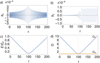Fig. 1. Ideal FMW-AW transformation with parameters Kx0 = 10, R = 0.1, and Ky = 0.1. Temporal evolution of (panel a) bx(τ), (panel b) by(τ), (panel c) the normalized total energy, E(τ)/E(0), and (panel d) wave frequencies (dispersion curves) of the FMW and the AW. In panel d the blue and orange lines denote the fast frequency and the Alfvén frequency, respectively. In all panels, the red dashed line marks τ*.

In addition to the FMW transferring part of its energy to the AW, the evolution of the wave energy in Figure 1c) evidences how the FMW exchanges energy with the flow. First, the wave energy decreases for τ < τ_* owing to a net flux of energy from the FMW to the background flow. Physically, this is caused by the shear flow attempting to reverse the direction of the FMW propagation. Then, K_x changes sign when τ = τ_*, producing the effective reflection of the FMW. For τ > τ_* the wave energy increases again, since now it is the flow that provides a net energy input to the FMW. In other words: the flow acts as a driver for the FMW. In the present linear model, the FMW energy increase happens indefinitely in time, because the stationary background flow is an infinite reservoir of energy. The time interval considered in Figure 1 is twice the value of τ_*, which makes the wave energy evolution to appear roughly symmetric with respect to τ = τ_*. However, the wave energy would continue to increase for later times.

Comparing our results to the ones presented in Figure 2 from Poedts et al. (1998), we can see that they are very similar to each other. It is easy to identify that the evolution of b_y(τ) from a FMW to an AW happens at the same τ and the final amplitude of the wave is the same. On the other hand it seems that our system ends up with slightly higher energy. Why this happens is unclear to us. It may be due to slight differences in the definition of the problem or some numerical inaccuracy in the solution of Poedts et al. (1998). We have been concerned to avoid numerical errors in the solutions. Nevertheless, comparing Figures 1b and 1c is obvious that outside of the DR, the energy is proportional to the fast frequency, Ω_F, as it is expected in the low shear case, assuring that our numerical method solves the problem correctly.

A peculiarity of such a system where only the FMW is initially generated and the evolution proceeds slowly, is that the energy transferred to the AW can be estimated from the change in the slope of the energy evolution (see Figure 1d). In this situation, as it has been commented earlier, the total energy of the system is proportional to the frequency of the FMW, E = λΩ_F, where λ determines the slope of the energy. As the incompressible AW cannot directly interact with the flow, the slope of energy evolution after τ = τ_* changes proportionally to the energy transmitted to the AW. The ratio of the slopes absolute value after and before τ = τ_*, computed as λ_a/λ_b, represents the fraction of initial energy that the FMW has preserved after the interaction with the AW, allowing us to approximately calculate the energy transferred to the AW as $E_A\approx E({\tau }_{\ast })(1-\frac{{\lambda }_a}{{\lambda }_b})$. In the case presented in Figure 1, the energy transmitted to the AW is around a 7.2% the total wave energy in the system at τ = τ_*, which corresponds to about 0.7% of the initial wave energy. Nevertheless, it is important to note that this provides a rough approximation of the transmitted energy and is only valid under slow evolution.

We used this example case as the reference for the rest of the studies performed in this work, namely a system with an initially pure FMW that partially transforms into an AW near the time, τ_*, obtained using the initial conditions b_x(0)≠0 and b_y(0) = b_x′(0) = b_y′(0) = 0.

3.1. Dependence on K_x0

We proceeded to study how the various parameters affect the solution, beginning with K_x0. We considered a system with K_y = 0.1 and R = 0.1, while we varied K_x0. All the considered cases meet the conditions presented in Section 2.3 for an effective coupling between the FMW and AW.

Figure 2 shows the results of the temporal evolution of the magnetic field perturbations for K_x0= 1, 10 and 15. In all cases, there is a partial transformation of the initially pure FMW into an AW around the time τ = τ_*, which depends on K_x0 (Equation (18)). For τ < τ_*, the b_x and b_y components of the magnetic field experience an amplification, while the amplitude of b_z decreases and becomes zero at τ = τ_*. As the total pressure perturbation is proportional to b_z, this indicates that the total pressure perturbation becomes zero just at τ = τ_*, when the mode conversion is most efficient. This can be understood by the fact that the AW generates no pressure perturbations. Conversely, for τ > τ_* the amplitudes of b_x and b_z progressively decrease and increase, respectively, while that of b_y, associated to the AW, remains constant since there is no further energy input to the AW after the DR.

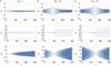Fig. 2. Ideal FMW-AW transformation with R = 0.1 and Ky = 0.1 for (a) Kx0 = 1, (b) Kx0 = 10, and (c) Kx0 = 15. From top to bottom, the temporal evolutions of bx(τ), associated with the FMW; by(τ), associated with the AW; and bz(τ), related to the total pressure perturbation, are respectively displayed. The red dashed line marks τ* in all plots.

As shown in Figure 3, the value of K_x0 determines the initial FMW frequency (Equation (29a)). Varying K_x0 produces a shift in the temporal evolution of the frequencies, modifying linearly the time required for the waves to reach the DR according to Equation (18). However, the rate at which the FMW frequency evolves due to the flow remains constant, although the rate of energy exchange varies for each case. This can be seen in Figure 4, which displays the temporal dependence of the wave energies. Due to the different slopes that the FMW energy curves have for the various values of K_x0, and the different amplitudes of the resulting AW energies, we find that the smaller K_x0, the higher the efficiency of energy transmission from the FMW to the AW, and the earlier this coupling happens.

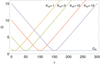Fig. 3. Dispersion curves (wave frequencies versus time) of the FMW (solid lines) and the AW (dashed line) for R = 0.1, Ky = 0.1, and various values of Kx0 indicated next to each line. The AW frequency is the same in all cases.

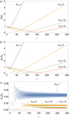Fig. 4. Ideal FMW-AW transformation with R = 0.1, Ky = 0.1, and various values of Kx0 indicated within the panels. Temporal evolution of (panel a) normalized total energy, E(τ)/E(0); (panel b) normalized FMW energy contribution, EF(τ)/E(0); and (panel c) nomalized AW energy contribution, EA(τ)/E(0).

To understand this result, let us compare the total energy evolution (Figure 4a), with the respective frequency evolution (Figure 3). It becomes evident that the relation E ∝ Ω holds true outside the DR, which is consistent with the expected behavior of slowly evolving wave modes. Furthermore, its clear that the value of K_x0 modifies the proportionality constant between the energy and frequency, resulting in smaller slopes in the energy evolution for larger K_x0. The case with K_x0 = 1 must be highlighted, since it is already located within the DR at the beginning of the evolution, but maintains the relation E ∝ Ω outside of it. The difference in τ_* of the cases with different K_x0 implies that systems with larger K_x0 take longer to reach the DR. This means that the larger the value of K_x0, more time the FMW has to give energy to the flow, and the lower the FMW energy is when the interaction with the AW begins, as can be observed in Figure 4a, resulting in a smaller amount of energy transferred to the AW. Hence, the larger K_x0 is, the less energy that is transmitted to the AW, as can be seen in Figure 4c.

Figure 5 shows the fraction of energy transmitted to the AW as a function of K_x0. The efficiency of the energy transmission primarily follows an overall decreasing tendency with increasing K_x0, except in the proximity of K_x0 ≈ 1 where the AW energy fraction reaches a maximum of 5%, approximately. We recall that the case with K_x0 = 1 corresponds to a system where the DR is initially realized. Surprisingly, we find an energy transference of ∼2.5% when K_x0 → 0. This behavior may be unexpected, as one might not anticipate any energy transference at all when K_x0 = 0. However, due to the effect produced by the shear flow, the effective wave number in the x direction, K_x(τ) = K_x0 − Rτ, does not remain null throughout the temporal evolution and there is always some partial wave transformation when K_x ≠ 0.

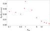Fig. 5. Fraction of energy transmitted to the AW as a function of Kx0 for an ideal FMW-AW transformation with R = 0.1 and Ky = 0.1.

3.2. Dependence on K_y

Here we study the effect of K_y. The value of this wave number component is very important for the wave coupling even in the absence of flow. Gogoberidze et al. (2004) derived some analytical approximations of transformation coefficient for the FMW-AW coupling, T_FA, that informs of how much energy is transmitted between modes as the system traverses the DR. The approximations were done in the low-β regime and as functions of the parameter δ = K_y/R^1/3. When δ ≫ 1, the approximated transformation coefficient between FMW and AW is

$$\begin{array}{c}\hfill T_{\mathit{FA}}\approx \frac{\pi }{2}exp(-\frac{K_y^3}{3R}),\end{array}$$(32)

whereas when δ ≪ 1, the transformation coefficient can be approximated by

$$\begin{array}{c}\hfill T_{\mathit{FA}}\approx \frac{2^{2/3}\pi K_y}{3^{1/3}\mathrm{\Gamma }\left(\frac{1}{3}\right)R^{1/3}}(1-\frac{\mathrm{\Gamma }\left(\frac{1}{3}\right)}{2^{7/4}{3}^{1/3}\mathrm{\Gamma }\left(\frac{2}{3}\right)}\frac{K_y^4}{R^{4/3}}),\end{array}$$(33)

where Γ is the so-called gamma function. Expressions (32) and (33) fail when δ ∼ 1 and so K_y ∼ R^1/3. Despite this, Equation (33) may be used to roughly calculate the critical K_y for which the energy transmission is maximal, namely

$$\begin{array}{c}\hfill K_{\mathrm{ycr}}={\left(\frac{2^{7/4}{3}^{1/3}\mathrm{\Gamma }\left(\frac{2}{3}\right)}{5\mathrm{\Gamma }\left(\frac{1}{3}\right)}\right)}^{1/4}{R}^{1/3},\end{array}$$(34)

which is used as a reference in this study. We recall that Equations (32)–(34) are taken from Gogoberidze et al. (2004), where all the details about their derivation can be found.

With all of this in mind, we then considered a system with K_x0 = 10 and R = 0.1. According to Equation (34), the critical K_y is K_ycr ≈ 0.39. We computed numerical solutions of this system for differnt values of K_y. We also considered the case with K_y = 0 for which the FMW and the AW become uncoupled, resulting only in the interaction between the FMW and the background flow. The variation of the initial FMW frequency with K_y is negligible since K_x0 ≫ K_y in all considered cases. In addition, all cases keep the same critical time for the DR realization, τ_* = 100, and the same initial energy.

Figure 6 shows the temporal evolution of b_x and b_y, and Figure 7 shows the corresponding energy evolution for K_y = 0, K_y = K_ycr = 0.39, and K_y = 0.8. As can be seen in Figure 7, when K_y = 0, no energy is transmitted to the AW, and the FWM just experiences the evolution caused by the shear flow: It transfers energy to the background flow until τ = τ_*, when the flow produces its reflection, and extracts energy back from the flow afterward. Since there is no energy interchanged with the AW in this case, the rate of energy transfer between the flow and the FMW is the same before and after the DR, but the energy flux is reversed, meaning that the FMW regains its initial energy at a time of τ = 2τ_*.

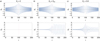Fig. 6. Ideal FMW-AW transformation with R = 0.1 and Kx0 = 10 for (a) Ky = 0, (b) Ky = Kycr = 0.39, and (c) Ky = 0.8. Top and bottom panels display the temporal evolutions of bx(τ) and by(τ), respectively. The red dashed line marks τ* in all plots.

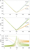Fig. 7. Same as Figure 4 but with R = 0.1, Kx0 = 10, and various values of Ky indicated within the panels.

When we consider K_y ≠ 0 but still K_y ≪ 1, the effects of the coupling between waves begin to appear, but they are weak, resulting only in small-scale perturbations in the Alfvén components. When larger values of K_y are considered, the coupling becomes more important, increasing the energy transferred to the AW. As K_y approaches K_ycr, where the maximum energy transfer between waves occurs, the perturbations begin to display mixed wave behaviors from τ = τ_* onward. Since a larger fraction of the energy goes to the AW, which cannot interact with the flow, there is a decrease in the efficiency at which the FMW extracts energy from the flow for τ > τ_*, as can be seen from Figure 7a, and b. As K_y keeps increasing from K_ycr, the FMW and the AW begin to decouple, as the value of K_y now has a non-negligible contribution to the FMW frequency at τ = τ_*. Since the FMW frequency and the AW frequency are no longer equal at τ = τ_*, a true DR cannot be realized. As a consequence of that, the energy transmitted to the AW decreases as K_y further increases from K_ycr.

For K_y < K_ycr, the energy feedback from the AW to the FMW is irrelevant, meaning that all the energy transmitted to the AW is retained in that oscillation mode. This is no longer true for K_y ≳ K_ycr. In the temporal evolution of the AW energy (Figure 7c), we observe a pulse-like phenomenon around τ = τ_*, before the system reaches its final energy state. For small K_y, the pulse has a very small amplitude and minimal impact on wave evolution. However, as K_y increases, the amplitude of the pulse grows and, consequently, the feedback of the AW on the FMW becomes more significant. This is evident in the emergence of some mixed wave behaviors in the perturbations (Figure 6).

When K_y takes large values, another feature begins to appear in the temporal evolution of the waves. It is evident in Figure 6 that for K_y = 0.8 the b_x amplification around τ = τ_* becomes truncated by a sudden amplitude decrease. This phenomenon is accompanied by an increase in the amplitude of b_y, during which the b_y oscillation has the frequency of the FMW rather than that of the AW. This coincides with a maximum in the energy transmitted to the AW, after which the AW quickly returns a fraction of its energy back to the FMW and recovers its characteristic AW frequency. This feature of the transformation becomes more pronounced as the value of K_y rises.

An analysis of the fraction of energy transmitted to the AW as a function of K_y has been conducted. In Figure 8, the results obtained from the numerical calculations are compared to the transformation coefficients of Gogoberidze et al. (2004), given in Equations (32) and (33). The square of the analytical coefficients are plotted, since they are transformation coefficients for the wave amplitude and the energy depends quadratically on the amplitudes. Moreover, the coefficients need to be scaled by multiplying them by a constant to correctly match the numerical data. It is clear from Figure 8 that the analytical coefficients fit the tendency of the numerical results reasonably well in their corresponding range of applicability, but significant discrepancies appear when K_y ≈ K_ycr. Nevertheless, the utility of the analytical approximations of the transmission coefficients derived by Gogoberidze et al. (2004) is evident. As expected, the energy transmission to the AW is maximal when K_y = K_ycr and is ∼5% the initial wave energy.

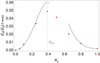Fig. 8. Fraction of energy transmitted to the AW as a function of Ky for an ideal FMW-AW transformation with R = 0.1 and Kx0 = 10. The red points correspond to the numerical results, while the blue lines are the approximated transmission coefficients from Gogoberidze et al. (2004). The vertical dashed line denotes Kycr.

3.3. Dependence on R

Finally in this ideal case, we study the dependence on the normalized strength of the velocity shear, R. We consider K_x0 = 10 and K_y = 0.1, while R is varied. Figures 9 and 10 display the evolution of the perturbations (b_x and b_y) and the wave energies, respectively, for R = 0, 0.1, and 0.2, with the energy plot also showing an additional result for R = 0.5. The shearless scenario with R = 0 is included as a reference, as there are no effects due to the flow and no energy exchange between waves. The excitation of the AW is minimal in the shearless case and is only caused by the fact that K_y ≠ 0.

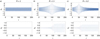Fig. 9. Ideal FMW-AW transformation with Kx0 = 10 and Ky = 0.1 for (a) R = 0, (b) R = 0.1, and (c) R = 0.2. Top and bottom panels display the temporal evolutions of bx(τ) and by(τ), respectively. The red dashed line marks τ* in all plots.

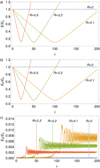Fig. 10. Same as Figure 4 but with Kx0 = 10, Ky = 0.1, and various values of R indicated within the panels.

When R ≠ 0, there is partial transformation of the FMW into the AW. The time for the DR realization, τ = τ_*, depends on R accoding to Equation (18). Hence, the larger R, the smaller τ_*. In contrast with what happens when K_x0 is varied, where a temporal shift of the whole evolution is found, now there is no change in the initial FMW frequency, when R changes, and the time scale of energy exchange between background flow and the FMW is affected. This can be better seen by comparing Figures 3 and 11. In the latter it is seen that the larger R, the steeper the frequency slope. This agrees with the discussion in Section 2.3 where it is noted that the time scale of the energy exchange between the waves and the flow is of the order of ∼R⁻¹.

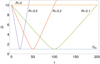Fig. 11. Same as Figure 3 but with Kx0 = 10, Ky = 0.1, and various values of R indicated within the figure.

The time scale of interaction between waves within the DR also changes with the value of R, since the rate of change of K_x(τ) is proportional to R. Specifically, the larger R, the shorter the time spent in the DR. This may conflict with the condition of “slow passing” through the DR if R is large enough, thereby reducing the efficiency of energy transfer between waves. This behavior is confirmed in Figure 10c, where the energy transmitted to the AW decreases as the value of R increases, and it becomes even clearer in the energy analysis of Figure 12. We found that the energy transference grows as R increases from R = 0 until a maximum is reached around R ≈ 1.5 × 10⁻³, where the energy transfer to the AW is 5% of the initial energy, approximately. From this point, the energy transferred to the AW begins to decrease rapidly as R keeps increasing. The occurrence of the maximum is caused by the competition of two already discussed temporal scales, namely the time of energy exchange between the flow and the FMW (that decreases with increasing R) and the time spent in the DR.

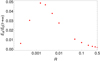Fig. 12. Fraction of energy transmitted to the AW as a function of R for an ideal FMW-AW transformation with Kx0 = 10 and Ky = 0.1.

Lastly, special attention has to be paid to the case with R = 0.5, which may not meet the condition of low shear. However, the results show that the energy follows closely the relation E ∝ Ω when the system is outside the DR. Additionally, the behavior of the perturbations b_x and b_y (not shown here) display a consistent behavior with the rest of the studied cases. This suggests that the approximation E ∝ Ω can be applied successfully over a wider range of R values beyond the strict low shear limit.

4. FMW-AW transformation with ambipolar diffusion

Now that we have a clear picture on how the mode coupling process behaves in the ideal case, we introduce the effect of ambipolar diffusion, so that ${\stackrel{\sim }{\eta }}_A\ne 0$. We retain ε = 0 to study the FMW-AW transformation alone. These conditions reduce Equations (10) to

$$\begin{array}{cc}& {\psi }^{(2)}-{\stackrel{\sim }{\eta }}_{A}R(2+4K_x^2+K_y^2)b_x-3{\stackrel{\sim }{\eta }}_{A}R{K}_x{K}_y{b}_y\hfill \\ \hfill & +{\stackrel{\sim }{\eta }}_A{K}_x(1+K_x^2+K_y^2)b_x^{(1)}+{\stackrel{\sim }{\eta }}_A{K}_y(1+K_x^2+K_y^2)b_y^{(1)}=0,\hfill \end{array}$$(35a)

$$\begin{array}{cc}& b_x^{(2)}+{\stackrel{\sim }{\eta }}_A(1+K_x^2)b_x^{(1)}+(1+K_x^2-2{\stackrel{\sim }{\eta }}_{A}R{K}_x)b_x\hfill \\ \hfill & +{\stackrel{\sim }{\eta }}_A{K}_x{K}_y{b}_y^{(1)}+(K_x{K}_y-{\stackrel{\sim }{\eta }}_{A}R{K}_y)b_y=0,\hfill \end{array}$$(35b)

$$\begin{array}{cc}& b_y^{(2)}+{\stackrel{\sim }{\eta }}_A(1+K_y^2)b_y^{(1)}+(1+K_y^2)b_y\hfill \\ \hfill & +{\stackrel{\sim }{\eta }}_A{K}_x{K}_y{b}_x^{(1)}+(K_x{K}_y-{\stackrel{\sim }{\eta }}_{A}R{K}_x)b_x=0,\hfill \end{array}$$(35c)

which describe the interaction between the FMW and the AW, but now adding the ambipolar diffusion. Contrary to what happens in the ideal System (28), the equation for ψ (Equation (35a)) cannot be discarded, as it becomes coupled with b_x and b_y through the ambipolar diffusion terms. However, b_x and b_y remain uncoupled to ψ because in Equations (35b) and (35c) there are no terms with ψ. Therefore, the evolution of ψ affects neither the FMW nor the AW, which means that for some of the calculations it is enough to consider the latter two equations alone. Conversely, the waves would drive perturbations in ψ, i.e., perturbations in density, which can be computed afterward from the first equation once b_x and b_y are known.

As the diffusion terms are presumably small for physical conditions in the partially ionized solar plasma (see, e.g., Khodachenko et al. 2004; Soler 2024), we may still use the fundamental frequencies for the ideal case (Equation (29)) as approximations for the frequencies of the waves in the presence of dissipation. Furthermore, the energy of the waves can still be computed with the expressions in Equation (30), as the change in the amplitude of the perturbations themselves account for the diffusion-related damping.

The setup we analyze here is equivalent to the one studied in the ideal scenario of an initially pure FMW that partially transforms to an AW, obtained using the initial conditions b_x(0) = 1, and b_y(0) = b_x′(0) = b_y′(0) = 0. Concerning the conditions for ψ, we use ψ(0) = K_x0b_x(0) and ψ′(0) = 0, thus ensuring that the initial density perturbation is zero. As system parameters we take K_x0 = 10, K_y = 0.1 and R = 0.1, which result in τ_* = 100. The dimensionless diffusion coefficient, ${\stackrel{\sim }{\eta }}_A$, is taken as a free parameter.

Figure 13 shows the evolution of the magnetic field perturbations b_x, b_y, and b_z for ${\stackrel{\sim }{\eta }}_A={10}^{-4}$ and ${\stackrel{\sim }{\eta }}_A={10}^{-3}$. Additionally, the solutions in the ideal case (obtained with ${\stackrel{\sim }{\eta }}_A=0$) are shown as a reference. The first effect we observe is the expected decrease of the waves amplitude for large times when ambipolar diffusion is present. The waves exhibit a faster damping as ${\stackrel{\sim }{\eta }}_A$ increases. Valuable information is provided by the analysis of the energy evolution in Figure 14. The observed damping of the perturbations is accompanied by a dissipation of wave energy. A consequence of the energy dissipation is a change of the behavior of the energy temporal evolution since, as commented earlier, in the last lines of Subsect. 2.3, we now have $E\propto ̸\mathrm{\Omega }$. The difference between the FMW energy evolution in the ideal case and that with diffusion becomes substantial at large times, and the larger ${\stackrel{\sim }{\eta }}_A$, the earlier this difference arises. Another property of the total energy evolution is that it saturates to a constant value for large times and this saturation value gets larger as ${\stackrel{\sim }{\eta }}_A$ increases. This feature of the energy evolution is caused by a new effect that is absent from the ideal scenario and appears when ambipolar diffusion is present. This new effect is analyzed later in the final paragraphs of this Section.

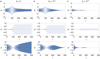Fig. 13. Dissipative FMW-AW transformation with R = 0.1, Kx0 = 10, and Ky = 0.1 for (a) ${\stackrel{\sim }{\eta }}_A=0$, (b) ${\stackrel{\sim }{\eta }}_A={10}^{-4}$, and (c) ${\stackrel{\sim }{\eta }}_A={10}^{-3}$. From top to bottom the temporal evolutions of bx(τ), by(τ), and bz(τ) are respectively displayed. The red dashed line marks τ* in all plots.

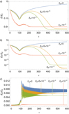Fig. 14. Same as Figure 4 but for a dissipative FMW-AW transformation with R = 0.1, Kx0 = 10, Ky = 0.1, and various values of ${\stackrel{\sim }{\eta }}_A$ indicated within the panels.

Concerning the FMW-AW conversion around τ = τ_*, we reach the following conclusions. In the first place, because of the presence of diffusion, the FMW dissipates part of its energy before reaching the DR. This results in a reduction of the available energy to be transmitted to the AW. For the largest considered value of ${\stackrel{\sim }{\eta }}_A={10}^{-3}$, the energy transferred to the AW is negligible. This occurs because the FMW damping happens so fast that almost all the FMW energy has already been dissipated before reaching the DR. Secondly, in Figure 14c) it might appear that, after the mode conversion, the AW energy stays unaffected by the diffusion as it seems to reach a constant value for large times. Detailed investigation reveals that there is indeed diffusion in the AW, but it occurs at a much slower pace compared to that of the FMW. This behavior is related to the different damping time scales that the MHD waves have in the presence of ambipolar diffusion (see Soler 2024). The AW damping rate depends only on the parallel component of the wave number, k_z, which remains constant throughout the evolution, while that of the FMW depends on the wave number modulus, which increases with time owing to the effect of the shear flow on K_x. At a sufficiently large time, when the wave number modulus is large enough, the FMW becomes much more efficiently damped than the AW.

In the ideal case, for τ > τ_* the shear flow provides an unlimited input of energy to the reflected FMW. Now we find that ambipolar diffusion impairs the ability of the flow to give energy to the FMW. Owing to the growing efficiency of the ambipolar damping with time, the FMW energy increase stops when the energy dissipation rate becomes equal than the energy extraction rate from the flow, and decreases afterward. In Figure 14 it is easy to see that this maximum in the energy evolution shifts to smaller times as ${\stackrel{\sim }{\eta }}_A$ increases. A study on how the value of ${\stackrel{\sim }{\eta }}_A$ affects the maximum energy and the time needed to reach it has been carried out by considering a wide range of ${\stackrel{\sim }{\eta }}_A$. The results (not shown here for simplicity) confirm a decreasing trend in the maximum energy and the corresponding times at which the maximum is attained with increasing ${\stackrel{\sim }{\eta }}_A$.

As commented earlier, it is found that the wave energy saturates to a constant value at large times when ambipolar diffusion is present (see Figure 14). This is caused by a new effect related to the appearance of a constant flow along the z-direction as a consequence of the diffusion. This additional flow originates from the equation for ψ (Equation (35a)), which was uncoupled in the ideal case. However, perturbations are now driven in ψ due to a diffusion-induced coupling. Perturbations in ψ are associated with density perturbations in an effect akin to having a pressure gradient along the z-axis. That, in turn, drive velocity perturbations in the z-direction. This becomes evident when examining the evolution of u_z in Figure 15, showing that the mean value of u_z at large times is zero in the ideal case but nonzero in the ambipolar case. This constant flow increases with the value of ${\stackrel{\sim }{\eta }}_A$.

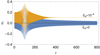Fig. 15. Temporal evolution of uz(τ) in the ideal case (blue line) and in a dissipative case with ${\stackrel{\sim }{\eta }}_A={10}^{-4}$ (orange line) for a FMW-AW transformation with R = 0.1, Kx0 = 10, and Ky = 0.1.

To further explore the nature of this constant longitudinal flow driven by diffusion, we have extended the investigation by considering the case with gas pressure (ε ≠ 0) and have reexamined some of the computations. These results are not included here and are to be explored in detail in the forthcoming continuation of this paper, where the case ε ≠ 0 will be investigated at length. However, we feel it convenient to anticipate these findings as they are crucial to understand the diffusion-induced flow found here.

When ε ≠ 0, it turns out that this constant longitudinal flow driven by diffusion is absent from the results. Instead, the energy that would be transferred to this longitudinal flow is invested in exciting the SMW, which is present in the system when ε ≠ 0. Thus, it becomes clear that the true nature of this constant flow we obtain here is to produce a new coupling with the SMW mediated by ambipolar diffusion that has no equivalence in the ideal case. To the best of our knowledge, this has not been reported before in the literature. The SMW cannot be driven in the present computations with ε = 0, but the coupling mechanism remains somehow in the form of this constant flow. This result shows that the general ε ≠ 0 case needs to be considered to fully understand the coupling between the MHD waves in the ambipolar case. Its comprehensive study is beyond the scope of this initial paper and is left for the second part.

5. Application to solar prominences

We perform a specific application to solar prominences in order to explore the FMW-AW transformation and energy transference that may happen in these structures. Solar prominences are large structures of relatively cool and dense plasma suspended in the solar corona. The prominence plasma has physical conditions similar to those found in the chromosphere (see, Vial & Engvold 2015). This is partially ionized plasma with a temperature in the range of 7000–9000 K. Prominences are composed of a myriad of thin threads that outline particular field lines of their magnetic structure (see, Lin 2011; Martin 2014). It has been shown that transverse MHD waves are ubiquitous in the fine threads (see, e.g., Lin et al. 2009; Ballester 2015; Arregui et al. 2018), and there is evidence suggesting that the waves originate at the photosphere (Hillier et al. 2013). Alfvénic waves driven at the photosphere can transport a substantial amount of energy to coronal heights (see Soler et al. 2019).

We considered a simple model of a thin thread with a length² of L_T = 3 × 10⁶ m and a radius an order of magnitude lower, R_T = 1.5 × 10⁵ m, with a temperature of T = 8000 K, a density of ρ = 5 × 10⁻¹¹ Kg m⁻³, and a magnetic field strength of B₀ = 10 G. The Alfvén speed is V_A ≈ 126 km s⁻¹. The ambipolar diffusion coefficient of the plasma in the thread is η_A = 5.4 × 10⁷ m² s⁻¹. This value has been adopted from the prominence thread models of Melis et al. (2023), where the details of the calculation can be found. The dimensionless ambipolar diffusion coefficient is ${\stackrel{\sim }{\eta }}_A\approx 4.5\times {10}^{-4}$.

The wave number components k_z and k_x0 are related to the physical dimensions of the thread as k_z = π/L_T ≈ 1.05 × 10⁻⁶ m⁻¹ and k_x0 = π/R_T ≈ 1.05 × 10⁻⁵ m⁻¹, resulting in a dimenssionless K_x0 = k_x0/k_z = 10. To calculate the normalized strength of the velocity shear, R, we assume typical flow velocities in solar prominences (see, e.g., Zirker et al. 1998) and take a variation of the flow velocity across the thread of 10 km s⁻¹, resulting in A = 1/30 s⁻¹ and thus R ≈ 0.252. The value of K_y is arbitrary and we study two situations, K_y = 0.1K_x0 = 1 and K_y = K_x0 = 10, corresponding to a kink mode and a high fluting mode, respectively, in the cylindrical equivalent to this Cartesian configuration. The value of K_ycr according to Equation (34) is K_ycr ≈ 0.53, which is smaller than the two considered values but relatively close to the kink case.

With all that, we have τ_* ≈ 40. We can reassign dimensions to this characteristic time to determine the physical time scale of the mode conversion and find t_* ≈ 300 s. In other words, the temporal scale of the energy exchange between background flow and wave modes is approximately 5 minutes. This is of the same order as the periods of the observed transverse oscillations in threads (see, e.g., Lin et al. 2009), which indicates that the shear-flow-driven wave coupling may be relevant in these structures.

A notable aspect of this application is the significant differences between the FMW frequencies of the two cases with different K_y. This is evident in the dispersion curves shown in Figure 16. The case with K_y = 1 presents a dispersion curve quite similar to the theoretical cases studied earlier, with a FMW frequency that becomes very close to the AW frequency when τ ∼ τ_*, hence ensuring there will be some coupling and energy transference between wave modes. Conversely, in the case with K_y = 10 the initial FMW frequency is higher and never approaches the AW frequency sufficiently, which is an essential condition for the DR realization. Therefore, using again the cylindrical equivalent to this Cartesian case, we speculate that an efficient coupling may happen for kink modes but not for fluting modes in threads modeled as cylindrical flux tubes.

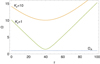Fig. 16. Dispersion curves (wave frequencies versus time) of the FMW (solid lines) and the AW (dashed line) for the parameters used in the application of Section 5.

The temporal evolution of the magnetic field perturbations are displayed in Figure 17. The aspect that stands out most in these results is the great difference the temporal evolution presents between both cases, as was expected. On the one hand, when K_y = 1 it is easy to see the typical temporal evolution of an initial FMW that partially transforms into an AW around τ = τ_*, for a case with a value of K_y higher than the K_ycr, but not large enough for the shear coupling not to be the primary coupling mechanism between both wave modes. We find in the b_x component the initial amplification of the FMW up to τ ∼ τ_*, at which point this amplification is truncated due to the momentary coupling and energy transfer between the waves that happens within the DR. This is followed by the strong damping of the FMW by the ambipolar diffusion for τ > τ_*. The FMW is completely damped around τ ≈ 140, which corresponds to a physical time of 17.5 minutes, approximately. The AW also presents a temporal evolution consistent with expectations in this case, with an amplification of the b_y component up to τ ∼ τ_*, where the b_y component becomes primarily Alfvénic. During the wave-wave interaction around the DR, a small fraction of the energy transferred to the AW is returned back to the FMW, evidenced by the sudden drop in amplitude of b_y just after τ = τ_*. Then, b_y remains with an almost constant amplitude, slowly decrasing because of the weak ambipolar damping. Thus, in summary, the evolution exhibits some mixed wave behavior after and during the DR realizarion, but loses all FMW character shortly after surpassing the DR. This is expected, as the ambipolar damping time of the FMW is much shorter than that of the AW

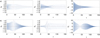Fig. 17. Dissipative FMW-AW transformation for the solar prominence thread conditions of Section 5 with a) Ky = 10 and b) Ky = 1. From left to right, the temporal evolution of bx(τ), by(τ), and bz(τ) are respectively displayed. The red dashed line marks τ* in all plots.

On the other hand, the case with K_y = 10 shows a completely different temporal evolution. To begin with, the larger value of K_y makes the waves to have mixed properties from the beginning of the evolution. Both b_x and b_y display oscillations with a high frequency (the FMW frequency) overlaying a lower one (the AW frequency). Additionally, the effects of shear flow coupling are much more subtle than in the previous case, noticeable mainly through the change in the frequency of the b_x component or the small change in amplitude in the b_y component. These effects are completely absent from the b_z component. However, the effects of ambipolar diffusion are stronger than in the previous K_y = 1 case. We observe that the FMW component of the oscillation, with a much higher frequency than in the previous case, becomes completely damped for a time around τ ∼ 100, corresponding to 12.5 minutes in physical time, a shorter time scale than the obtained when K_y = 1. This reassures the conclusion that the larger the wave number, the faster the FMW is damped because of ambipolar effects. Later, for τ > 100, the b_x perturbation becomes a slowly damped wave of predominantly Alfvénic character, the b_y perturbation also becomes an Alfvénic wave but with an almost constant amplitude, and the b_z perturbation is completely damped as the FMW is fully dissipated by the ambipolar diffusion.

The differences between both cases also become evident from the energy temporal evolution displayed in Figure 18. The first noticeable aspect is the absence of a local energy minimum around τ = τ_* in the total energy curve of the K_y = 10 case, as opposed to the case with K_y = 1. Additionally, the dissipation of energy is faster in the case with larger K_y, despite maintaining a larger amount of residual energy associated with the longitudinal flow induced by ambipolar diffusion.

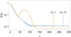Fig. 18. Temporal dependence of the normalized total energy, E(τ)/E(0), in the dissipative FMW-AW transformation for the solar prominence thread conditions of Section 5 with Ky = 1 (orange line) and Ky = 10 (blue line).

We conclude this application by summarizing some important points. Firstly, we found that the coupling and energy exchange between FMW and AW is possible in prominence threads and other similar structures, such as chromospheric spicules. Secondly, due to the ambipolar diffusion, the FMW have a much shorter lifespan than the AW, which persist for longer times. This is caused by the effect of the shear flow on the effective normal wave number, K_x. As K_x increases (in absolute value) for large times, diffusion becomes more and more efficient for the FMW. Lastly, we observed that for large K_y the shear-induced wave coupling loses relevance, but it is important for K_y values consistent with kink modes.

6. Concluding remarks

We have shown that the energy exchanges and wave-wave interactions arising in a plasma with a shear flow are complex processes that are governed by multiple factors related to both the waves and the flow. The situation becomes even more complex when a dissipative effect, such as ambipolar diffusion, is included. For instance, we find that ambipolar diffusion introduces a new coupling mechanism. Although the derived governing equations are general, we restricted ourselves to the FMW-AW transformation and conducted an exploratory investigation of how the shear flow and the ambipolar diffusion affects such a transformation. The model was applied to a situation representative of a prominence thread. We found that the conditions that occur in these structures are suitable for the coupling and energy exchange between waves. In view of the obtained results, we plan to investigate further in this direction. As this coupling has impacts on the evolution of the oscillations, it may be relevant to take its effects into account when interpreting the observations.

It is important to note that the analysis carried out in this work is linear in nature. Consequently, nonlinear effects, such as the variation of the flow due to the energy exchange between the waves and the flow are absent. Moreover, it should be recognized that considering these nonlinear effects may lead to substantial changes in the solutions as the flow itself evolves. Furthermore, while the nonmodal analysis is a valuable tool for obtaining solutions and describing the time evolution of the waves, it is essential to note that they are solutions in Fourier space. To obtain solutions in physical space, an inverse spatial Fourier transform is required. However, this is challenging due to the numerical nature of the results.

There are several paths to extending the investigations conducted here. The most immediate involves exploring the case with ε ≠ 0, as it introduces the SMW into the scene. Currently, our investigation on this is ongoing and will be presented in a follow-up of this paper. Analysis of the role of the Hall term is also of interest. In a future work, we may use nonlinear numerical simulations to consider the full problem beyond the linear analysis done here. To this end, the nonlinear numerical simulations of waves and flows in solar prominences by Ofman & Kucera (2020), Ofman et al. (2023) can be useful references.

Acknowledgments

This publication is part of the R+D+i project PID2023-147708NB-I00, funded by MCIN/AEI/10.13039/501100011033 and by FEDER, EU. This publication is part of the PREP2023-001251 grant, funded by MCIN/AEI/10.13039/501100011033 and the ESF+. RS would like to thank Marc Carbonell for his help with Mathematica and for obtaining some of the initial results.

References

All Figures

Fig. 1. Ideal FMW-AW transformation with parameters Kx0 = 10, R = 0.1, and Ky = 0.1. Temporal evolution of (panel a) bx(τ), (panel b) by(τ), (panel c) the normalized total energy, E(τ)/E(0), and (panel d) wave frequencies (dispersion curves) of the FMW and the AW. In panel d the blue and orange lines denote the fast frequency and the Alfvén frequency, respectively. In all panels, the red dashed line marks τ*.

In the text

	Fig. 2. Ideal FMW-AW transformation with R = 0.1 and Ky = 0.1 for (a) Kx0 = 1, (b) Kx0 = 10, and (c) Kx0 = 15. From top to bottom, the temporal evolutions of bx(τ), associated with the FMW; by(τ), associated with the AW; and bz(τ), related to the total pressure perturbation, are respectively displayed. The red dashed line marks τ* in all plots.
In the text

	Fig. 3. Dispersion curves (wave frequencies versus time) of the FMW (solid lines) and the AW (dashed line) for R = 0.1, Ky = 0.1, and various values of Kx0 indicated next to each line. The AW frequency is the same in all cases.
In the text

	Fig. 4. Ideal FMW-AW transformation with R = 0.1, Ky = 0.1, and various values of Kx0 indicated within the panels. Temporal evolution of (panel a) normalized total energy, E(τ)/E(0); (panel b) normalized FMW energy contribution, EF(τ)/E(0); and (panel c) nomalized AW energy contribution, EA(τ)/E(0).
In the text

	Fig. 5. Fraction of energy transmitted to the AW as a function of Kx0 for an ideal FMW-AW transformation with R = 0.1 and Ky = 0.1.
In the text

	Fig. 6. Ideal FMW-AW transformation with R = 0.1 and Kx0 = 10 for (a) Ky = 0, (b) Ky = Kycr = 0.39, and (c) Ky = 0.8. Top and bottom panels display the temporal evolutions of bx(τ) and by(τ), respectively. The red dashed line marks τ* in all plots.
In the text

	Fig. 7. Same as Figure 4 but with R = 0.1, Kx0 = 10, and various values of Ky indicated within the panels.
In the text

	Fig. 8. Fraction of energy transmitted to the AW as a function of Ky for an ideal FMW-AW transformation with R = 0.1 and Kx0 = 10. The red points correspond to the numerical results, while the blue lines are the approximated transmission coefficients from Gogoberidze et al. (2004). The vertical dashed line denotes Kycr.
In the text

	Fig. 9. Ideal FMW-AW transformation with Kx0 = 10 and Ky = 0.1 for (a) R = 0, (b) R = 0.1, and (c) R = 0.2. Top and bottom panels display the temporal evolutions of bx(τ) and by(τ), respectively. The red dashed line marks τ* in all plots.
In the text

	Fig. 10. Same as Figure 4 but with Kx0 = 10, Ky = 0.1, and various values of R indicated within the panels.
In the text

	Fig. 11. Same as Figure 3 but with Kx0 = 10, Ky = 0.1, and various values of R indicated within the figure.
In the text

	Fig. 12. Fraction of energy transmitted to the AW as a function of R for an ideal FMW-AW transformation with Kx0 = 10 and Ky = 0.1.
In the text

	Fig. 13. Dissipative FMW-AW transformation with R = 0.1, Kx0 = 10, and Ky = 0.1 for (a) ${\stackrel{\sim }{\eta }}_A=0$, (b) ${\stackrel{\sim }{\eta }}_A={10}^{-4}$, and (c) ${\stackrel{\sim }{\eta }}_A={10}^{-3}$. From top to bottom the temporal evolutions of bx(τ), by(τ), and bz(τ) are respectively displayed. The red dashed line marks τ* in all plots.
In the text

	Fig. 14. Same as Figure 4 but for a dissipative FMW-AW transformation with R = 0.1, Kx0 = 10, Ky = 0.1, and various values of ${\stackrel{\sim }{\eta }}_A$ indicated within the panels.
In the text

	Fig. 15. Temporal evolution of uz(τ) in the ideal case (blue line) and in a dissipative case with ${\stackrel{\sim }{\eta }}_A={10}^{-4}$ (orange line) for a FMW-AW transformation with R = 0.1, Kx0 = 10, and Ky = 0.1.
In the text

	Fig. 16. Dispersion curves (wave frequencies versus time) of the FMW (solid lines) and the AW (dashed line) for the parameters used in the application of Section 5.
In the text

	Fig. 17. Dissipative FMW-AW transformation for the solar prominence thread conditions of Section 5 with a) Ky = 10 and b) Ky = 1. From left to right, the temporal evolution of bx(τ), by(τ), and bz(τ) are respectively displayed. The red dashed line marks τ* in all plots.
In the text

	Fig. 18. Temporal dependence of the normalized total energy, E(τ)/E(0), in the dissipative FMW-AW transformation for the solar prominence thread conditions of Section 5 with Ky = 1 (orange line) and Ky = 10 (blue line).
In the text

References

- Arregui, I., Oliver, R., & Ballester, J. L. 2018, Liv. Rev. Sol. Phys., 15, 3 [Google Scholar]
- Ballester, J. L. 2015, in Solar Prominences, eds. J.-C. Vial, & O. Engvold, ASP Sci. Libr., 415, 259 [Google Scholar]
- Ballester, J. L., Alexeev, I., Collados, M., et al. 2018, Space Sci. Rev., 214, 1 [NASA ADS] [CrossRef] [Google Scholar]
- Bodo, G., Poedts, S., Rogava, A., & Rossi, P. 2001, A&A, 374, 337 [NASA ADS] [CrossRef] [EDP Sciences] [Google Scholar]
- Cally, P. S. 2001, ApJ, 548, 473 [Google Scholar]
- Cally, P. S., & Bogdan, T. J. 2024, in Magnetohydrodynamic Processes in Solar Plasmas, eds. A. K. Srivastava, M. Goossens, & I. Arregui, 99 [Google Scholar]
- Cally, P. S., & Gómez-Míguez, M. M. 2023, ApJ, 946, 108 [Google Scholar]
- Cally, P. S., & Khomenko, E. 2015, ApJ, 814, 106 [CrossRef] [Google Scholar]
- Cally, P. S., & Khomenko, E. 2018, ApJ, 856, 20 [Google Scholar]
- Cally, P. S., & Khomenko, E. 2019, ApJ, 885, 58 [Google Scholar]
- Camporeale, E. 2012, Space Sci. Rev., 172, 397 [Google Scholar]
- Chagelishvili, G., Hristov, T., Chanishvili, R., & Lominadze, J. 1993, Phys. Rev. E, 47, 366 [Google Scholar]
- Chagelishvili, G., Rogava, A., & Segal, I. 1994, Phys. Rev. E, 50, R4283 [Google Scholar]
- Chagelishvili, G., Rogava, A., & Tsiklauri, D. 1996a, Phys. Rev. E, 53, 6028 [Google Scholar]
- Chagelishvili, G., Chanishvili, R., & Lominadze, D. G. 1996b, J. Exp. Theor. Phys. Lett., 63, 543 [Google Scholar]
- Chagelishvili, G., Chanishvili, R., Lominadze, J., & Tevzadze, A. 1997, Phys. Plasma, 4, 259 [Google Scholar]
- De Pontieu, B., & McIntosh, S. W. 2010, ApJ, 722, 1013 [Google Scholar]
- Gogoberidze, G., Chagelishvili, G., Sagdeev, R., & Lominadze, D. 2004, Phys. Plasma, 11, 4672 [Google Scholar]
- González-Morales, P. A., Khomenko, E., & Cally, P. S. 2019, ApJ, 870, 94 [Google Scholar]
- González-Morales, P. A., Khomenko, E., Vitas, N., & Collados, M. 2020, A&A, 642, A220 [NASA ADS] [CrossRef] [EDP Sciences] [Google Scholar]
- Goossens, M., Erdélyi, R., & Ruderman, M. S. 2011, Space Sci. Rev., 158, 289 [Google Scholar]
- Hillier, A., Morton, R. J., & Erdélyi, R. 2013, ApJ, 779, L16 [Google Scholar]
- Khodachenko, M. L., Arber, T. D., Rucker, H. O., & Hanslmeier, A. 2004, A&A, 422, 1073 [NASA ADS] [CrossRef] [EDP Sciences] [Google Scholar]
- Khomenko, E., & Cally, P. S. 2019, ApJ, 883, 179 [Google Scholar]
- Khomenko, E., & Collados, M. 2012, ApJ, 747, 87 [Google Scholar]
- Khomenko, E., & Collados, M. 2015, Living Rev. Sol. Phys., 12, 6 [Google Scholar]
- Khomenko, E., Collados, M., Díaz, A., & Vitas, N. 2014, Phys. Plasmas, 21, 092901 [Google Scholar]
- Kotkin, G. L., & Serbo, V. G. 2013, Collection of Problems in Classical Mechanics: International Series of Monographs in Natural Philosophy (Elsevier), 31 [Google Scholar]
- Lin, Y. 2011, Space Sci. Rev., 158, 237 [Google Scholar]
- Lin, Y., Soler, R., Engvold, O., et al. 2009, ApJ, 704, 870 [NASA ADS] [CrossRef] [Google Scholar]
- Mahajan, S. M., & Rogava, A. D. 1999, ApJ, 518, 814 [Google Scholar]
- Martin, S. F. 2014, Solar Prominences (Springer), 205 [Google Scholar]
- Melis, L., Soler, R., & Terradas, J. 2023, A&A, 676, A25 [NASA ADS] [CrossRef] [EDP Sciences] [Google Scholar]
- Morse, P. M. 1981, Vibration and Sound (Woodbury, NY) [Google Scholar]
- Ofman, L., & Kucera, T. A. 2020, ApJ, 899, 99 [Google Scholar]
- Ofman, L., & Wang, T. J. 2008, A&A, 482, L9 [NASA ADS] [CrossRef] [EDP Sciences] [Google Scholar]
- Ofman, L., Kucera, T. A., & DeVore, C. R. 2023, ApJ, 944, 210 [Google Scholar]
- Okamoto, T. J., Tsuneta, S., Berger, T., et al. 2007, Science, 318, 1577 [Google Scholar]
- Pandey, B. P., & Wardle, M. 2008, MNRAS, 385, 2269 [Google Scholar]
- Poedts, S., Rogava, A. D., & Mahajan, S. M. 1998, ApJ, 505, 369 [Google Scholar]
- Poedts, S., Rogava, A., & Mahajan, S. 1999, Space Sci. Rev., 87, 295 [Google Scholar]
- Popescu Braileanu, B., & Keppens, R. 2021, A&A, 653, A131 [NASA ADS] [CrossRef] [EDP Sciences] [Google Scholar]
- Raboonik, A., & Cally, P. S. 2019, Sol. Phys., 294, 147 [Google Scholar]
- Raboonik, A., Tarr, L. A., & Pontin, D. I. 2024, ApJ, 967, 80 [Google Scholar]
- Rogava, A. D., & Mahajan, S. M. 1997, Phys. Rev. E, 55, 1185 [Google Scholar]
- Rogava, A. D., Mahajan, S., & Berezhiani, V. I. 1996, Phys. Plasmas, 3, 3545 [Google Scholar]
- Rogava, A. D., Chagelishvili, G. D., & Mahajan, S. M. 1998, Phys. Rev. E, 57, 7103 [Google Scholar]
- Rogava, A. D., Poedts, S., & Heirman, S. 1999, MNRAS, 307, L31 [Google Scholar]
- Schmid, P. J. 2007, Annu. Rev. Fluid Mech., 39, 129 [NASA ADS] [CrossRef] [Google Scholar]
- Soler, R. 2024, Phil. Trans. R. Soc. A, 382, 20230223 [Google Scholar]
- Soler, R., & Goossens, M. 2024, in Magnetohydrodynamic Processes in Solar Plasmas, eds. A. K. Srivastava, M. Goossens, & I. Arregui, 155 [Google Scholar]
- Soler, R., Oliver, R., & Ballester, J. L. 2009, ApJ, 707, 662 [NASA ADS] [CrossRef] [Google Scholar]
- Soler, R., Andries, J., & Goossens, M. 2012, A&A, 537, A84 [NASA ADS] [CrossRef] [EDP Sciences] [Google Scholar]
- Soler, R., Terradas, J., Oliver, R., & Ballester, J. L. 2016, A&A, 592, A28 [NASA ADS] [CrossRef] [EDP Sciences] [Google Scholar]
- Soler, R., Terradas, J., Oliver, R., & Ballester, J. L. 2017, ApJ, 840, 20 [Google Scholar]
- Soler, R., Terradas, J., Oliver, R., & Ballester, J. L. 2019, ApJ, 871, 3 [Google Scholar]
- Threlfall, J., Parnell, C. E., De Moortel, I., McClements, K. G., & Arber, T. D. 2012, A&A, 544, A24 [NASA ADS] [CrossRef] [EDP Sciences] [Google Scholar]
- Tian, H., McIntosh, S. W., Wang, T., et al. 2012, ApJ, 759, 144 [Google Scholar]
- Trefethen, L. N., Trefethen, A. E., Reddy, S. C., & Driscoll, T. A. 1993, Science, 261, 578 [Google Scholar]
- Vial, J.-C., & Engvold, O. 2015, Solar Prominences (Springer), 415 [Google Scholar]
- Walker, A. D. M. 2005, Magnetohydrodynamic Waves in Geospace (Institute of Physics Publishing), Ser. Plasma Phys. [Google Scholar]
- Zirker, J., Engvold, O., & Martin, S. 1998, Nature, 396, 440 [CrossRef] [Google Scholar]