| Issue |
A&A
Volume 701, September 2025
|
|
|---|---|---|
| Article Number | A289 | |
| Number of page(s) | 18 | |
| Section | Galactic structure, stellar clusters and populations | |
| DOI | https://doi.org/10.1051/0004-6361/202554258 | |
| Published online | 26 September 2025 | |
Stellar Population Astrophysics (SPA) with the TNG
Non-local thermodynamic equilibrium atmospheric parameters and abundances of giant stars in 33 open clusters★
1
INAF – Ossevatorio Astronomico di Padova,
vicolo dell’Osservatorio 5,
35122
Padova,
Italy
2
Department of Physics, University of Rome Tor Vergata,
via della Ricerca Scientifica 1,
00133
Rome,
Italy
3
Department of Astronomy & McDonald Observatory, The University of Texas at Austin,
2515 Speedway,
Austin,
TX
78712,
USA
4
INAF – Osservatorio di Astrofisica e Scienza dello Spazio di Bologna,
via P. Gobetti 93/3,
40129
Bologna,
Italy
5
Department of Physics and Astronomy, Monash University,
Clayton,
VIC 3800,
Australia
6
ARC Centre of Excellence for All Sky Astrophysics in 3 Dimensions (ASTRO 3D),
Australia
7
Center for Computational Astrophysics, Flatiron Institute,
162 5th Avenue,
New York,
NY
10010,
USA
8
Max Planck Institute for Astronomy,
Königstuhl 17,
69117
Heidelberg,
Germany
9
INAF – Osservatorio Astrofisico di Arcetri,
Largo E. Fermi 5,
50125
Firenze,
Italy
10
INAF – Ossservatorio Astrofisico di Catania,
via di S. Sofia 78,
95123
Catania,
Italy
11
INAF – Osservatorio Astronomico di Roma,
via Frascati 33,
00178
Monte Porzio Catone,
Italy
12
Fundacíon Galileo Galilei – INAF,
Rambla José Ana Fernández Pérez 7,
38712
Breña Baja,
Tenerife,
Spain
13
Faculty of Mathematics and Physics, University of Ljubljana,
Jadranska 19,
1000
Ljubljana,
Slovenia
★★ Corresponding authors: This email address is being protected from spambots. You need JavaScript enabled to view it.
; This email address is being protected from spambots. You need JavaScript enabled to view it.
Received:
25
February
2025
Accepted:
4
July
2025
Abstract
Context. Open clusters serve as important tools for accurately studying the chemical evolution of the Milky Way. By combining precise chemical data from high-resolution spectra with information on their distances and ages, we can effectively uncover the processes that have shaped our Galaxy.
Aims. This study aims to derive non-local thermodynamic equilibrium (NLTE) atmospheric parameters and chemical abundances for approximately one hundred giant stars across 33 open clusters with near-solar metallicity. The clusters span a wide range of ages, enabling an assessment of the presence and extent of any age-related abundance gradients.
Methods. In the Stellar Population Astrophysics (SPA) project, we acquired new high-resolution spectra of giant stars in a sample of open clusters using the HARPS-N echelle spectrograph at the Telescopio Nazionale Galileo. We chemically characterized nine open clusters for the first time and reanalyzed previously studied SPA clusters, resulting in a consistent and homogeneous sample.
Results. We determined NLTE atmospheric parameters using the equivalent width method and derived NLTE chemical abundances through spectral synthesis for various elements, including α elements (Mg, Si, and Ti), light odd-Z elements (Na, Al), iron-peak elements (Mn, Co, and Ni), and neutron-capture elements (Sr, Y, and Eu). We compared our findings with the existing literature, which revealed a good agreement. We examined the trends of [X/Fe] versus age, confirming previous observations and the enrichment patterns predicted by nucleosynthesis processes. Positive correlations with age are present for a elements such as Mg, Si, Ti, and odd-Z Al, and iron-peak elements Mn, Co, Ni, and Sr, while Na and neutron-capture Y and Eu show a negative trend. This study emphasizes the significance of NLTE corrections and reinforces the utility of open clusters as tracers of Galactic chemical evolution. Furthermore, we provide a benchmark sample of NLTE abundances for upcoming open cluster surveys within large-scale projects, such as 4MOST and WEAVE.
Key words: stars: abundances / stars: evolution / Galaxy: abundances / Galaxy: disk / Galaxy: evolution / open clusters and associations: general
Based on observations made with the Italian Telescopio Nazionale Galileo (TNG) operated on the island of La Palma by the Fundación Galileo Galilei of the INAF (Istituto Nazionale di Astrofisica) at the Observatorio del Roque de los Muchachos.
© The Authors 2025
 Open Access article, published by EDP Sciences, under the terms of the Creative Commons Attribution License (https://creativecommons.org/licenses/by/4.0), which permits unrestricted use, distribution, and reproduction in any medium, provided the original work is properly cited.
This article is published in open access under the Subscribe to Open model. This email address is being protected from spambots. You need JavaScript enabled to view it. to support open access publication.
1 Introduction
Open clusters (OCs) are groups of stars that originate from the same molecular cloud at practically the same time, and they therefore have similar ages, kinematics, and chemical compositions. As a single stellar population, their ages and distances can be estimated with great accuracy (Bragaglia & Tosi 2006; Bossini et al. 2019; Monteiro & Dias 2019; Cantat-Gaudin et al. 2020). Open clusters are ideal tracers of the structure of the Milky Way and have long been utilized to investigate the Galactic (thin) disk and its chemo-dynamical evolution over time (e.g., Janes 1979; Sestito et al. 2008; Magrini et al. 2009; Frinchaboy et al. 2013; Netopil et al. 2016; Casamiquela et al. 2017; Spina et al. 2021). Large spectroscopic surveys such as Gaia-ESO (Gilmore et al. 2012; Randich et al. 2013, 2022), GALAH (De Silva et al. 2015), APOGEE (Majewski et al. 2017), and LAMOST (Zhao et al. 2012), coupled with the high-quality data from the Gaia mission (Gaia Collaboration 2016, 2023a), have significantly improved our understanding of the OC population. As a result of the Gaia mission, a large number of OCs have been discovered and characterized, while many candidate clusters have been removed from the catalogs (see, e.g., Cantat-Gaudin et al. 2018; Castro-Ginard et al. 2019; Liu & Pang 2019; Hao et al. 2022; Castro-Ginard et al. 2020; Hunt & Reffert 2023). In the coming years, WEAVE (Dalton et al. 2018; Jin et al. 2024) and 4MOST (de Jong et al. 2019; Lucatello et al. 2023) will observe many more clusters at low and intermediate resolution (R ≈ 5000 and 20 000) and will provide new insights on their properties. Despite this, a significant portion of OCs remains unexplored in detail, particularly in terms of their chemical composition, limiting our ability to fully use these objects to probe the Galactic disk’s chemical and dynamical evolution.
The Stellar Population Astrophysics (SPA) is an ongoing project based on a Large Programme conducted at the Telescopio Nazionale Galileo (TNG) using the HARPS-N and GIANO-B echelle spectrographs over approximately 70 nights between 2018 and 2021. Within SPA, we acquired high-resolution spectra of stars near the Sun, covering a broad range of ages and properties. To improve our understanding of the Milky Way’s star formation and chemical enrichment history, the program focuses on several topics, such as mapping abundance gradients, cosmic spreads, and other irregularities in the abundances and ratios of individual elements within the Galactic disk. We specifically observed a selection of OCs by either targeting a few stars — mainly giants — in as many clusters as possible or by focusing on a larger number of stars — primarily main-sequence stars — in a smaller set of clusters. The primary goals of these observations were to determine the metallicity and detailed chemical composition across a broad sample of OCs, taking advantage of their nature as a single stellar population. This implies that even a single star can provide valuable insights into the entire cluster, although observing multiple members enhances the precision of key cluster parameters. Additionally, the project investigates how stellar properties relate to evolutionary stages, examining factors such as surface chemical variations caused by diffusion or mixing processes, as well as the evolution of stellar rotation and activity. Several papers have been published as part of the SPA project, analyzing either giant stars or main-sequence stars Frasca et al. (2019); D’Orazi et al. (2020); Casali et al. (2020a); Alonso-Santiago et al. (2021); Zhang et al. (2021, 2022); Fanelli et al. (2022); Vernekar et al. (2024).
In this paper, we present a homogeneous analysis of high-resolution spectra of 95 giant stars across 33 OCs, including nine clusters that are spectroscopically characterized for the first time by our team. Providing data for these previously understudied OCs is crucial for enhancing our understanding of the Galactic disk. We reanalyze giants from Casali et al. (2020a); Zhang et al. (2021, 2022), and Alonso-Santiago et al. (2021), and include giants from NGC 2632, previously examined by D’Orazi et al. (2020) within the SPA project focusing exclusively on main-sequence stars. By ensuring a homogeneous analysis of all spectra, we expand the SPA sample of OCs. Furthermore, while the previous analyses assumed local thermodynamic equilibrium (LTE) conditions, which may not be suitable for many elements and temperature or surface gravity ranges, we derive atmospheric parameters and abundances using a non-LTE (NLTE) approach.
The structure of the paper is as follows. Section 2 presents the observations and describes the selected sample of OCs. In Sect. 3, we outline the methods employed to determine stellar parameters and abundances. In Sect. 4, we present a comparison with the literature. Section 5 investigates the relationships between abundances and age gradients. Finally, Sect. 6 provides a summary of our findings and conclusions.
2 Observations and the cluster sample
The SPA Open Cluster program (SPA-OC) studies main-sequence and giant stars within OCs. The main-sequence stars in SPA are primarily located in younger, closer clusters, whereas red giants are typically observed in older and more distant clusters (within approximately 2 kpc of the Sun). In this work, we focus on evolved stars on the red giant branch (RGB) and red clump (RC). The targets were selected among the high-probability OC members based on Cantat-Gaudin et al. (2018, 2020), who relied on astrometry and photometry from Gaia Data Release 2 (DR2).
In this paper, we analyze the optical HARPS-N spectra, which have a resolution of R ≈ 115 000 and spectral coverage between 3800–6900 Å (Cosentino et al. 2012). The analysis and results based on GIANO-B near-infrared spectra are presented in a series of dedicated papers, for example, Bijavara Seshashayana et al. (2024a,b); Jian et al. (2024).
The observations discussed in this study were conducted between July 2018 and April 2023. The spectra were auto-matically reduced with the HARPS-N pipeline, which includes flat-field and bias corrections, wavelength calibration, extraction of 1D spectra, and corrections for barycentric motion. Exposure times varied depending on the star’s magnitude and sky conditions, and we combined the multi-exposure spectra before the analysis.
As mentioned above, our sample includes a total of 95 giant stars from 33 OCs. Table 1 lists their names, the number of stars per cluster, and basic parameters such as age, distance, Galactocentric distance, and extinction. The table also provides references for previous metallicity determinations based on high-resolution spectroscopy; for clusters with high-quality spectroscopy listed in Netopil et al. (2016), we do not provide references to the original papers. We note that some of these metallicities were not available at the time of observation (see, e.g., UBC 3, UBC 141, and UBC 577) and that some metallicities are based on low- or intermediate-resolution spectroscopy (see below).
Among the 33 OCs discussed in this study, 20 have previously been analyzed in SPA papers (Casali et al. 2020a; D’Orazi et al. 2020; Zhang et al. 2021, 2022; Alonso-Santiago et al. 2021); see references in Table 11. Four clusters have been reported in the literature by other authors, but are presented here for the first time in the context of the SPA project (see Fig. 1 and Table 1). Finally, this work provides the first metallicity determination based on high-resolution spectroscopy for nine OCs (NGC 6800, UBC 131, UBC 169, UBC 170, UBC 194 without metallicity values; and NGC 7086, UBC 60, UBC 141, UBC 577 with values based on low-resolution LAMOST or medium-resolution Gaia-RVS spectra).
The inclusion of the 20 OCs already studied within the SPA framework allows us to have a broader sample analyzed homogeneously and to extend the age range. These 33 OCs in the SPA sample are generally located close to the Galactic mid-plane and to the Sun (with an average Galactocentric distance of 8.6 kpc and RGC spanning from 7 kpc to approximately 10 kpc) and have ages ranging from about 40 Myr to 4 Gyr (see Table 1).
Figure 1 presents the color-magnitude diagrams based on Gaia DR3 photometric data for the 13 OCs that have not been included in previous SPA analyses. We also provide a brief description of these clusters in the following paragraphs.
IC 4756: This intermediate-age cluster (approximately 1.3 Gyr old according to Cantat-Gaudin et al. 2020; 970 Myr according to Bossini et al. 2019) is located very close to the Sun (≈500 pc) at a Galactocentric distance of ≈ 8 kpc. Several studies have assessed its metallicity, with some also investigating detailed elemental abundances (Jacobson et al. 2007; Santos et al. 2009; Smiljanic et al. 2009; Pace et al. 2010; Ting et al. 2012; Bagdonas et al. 2018; Casamiquela et al. 2017, 2019; Ray et al. 2022; Tsantaki et al. 2023; Carbajo-Hijarrubia et al. 2024). We identified eight stars in common with the existing literature, which are used later for comparison with our results (details can be found in Sect. 4).
NGC 752 (and Theia 1214): This cluster is located near the Sun and has an intermediate age of approximately 1.2 Gyr (Cantat-Gaudin et al. 2020) or 1.48 Gyr (Bossini et al. 2019). It has been extensively studied, particularly for lithium measurements (see, e.g., Boesgaard et al. (2022) and references therein). Other studies of metallicity and abundance include Sestito et al. (2004); Carrera & Pancino (2011); Reddy et al. (2012); Böcek Topcu et al. (2015); Casamiquela et al. (2017, 2019); Lum & Boesgaard (2019); Spina et al. (2021); Myers et al. (2022); Donor et al. (2020); Carbajo-Hijarrubia et al. (2024). The cluster shows signs of either dynamical or tidal dispersal (Carraro et al. 2014) and features long, asymmetric tidal tails extending over 260 pc on the sky (Bhattacharya et al. 2021; Boffin et al. 2022; Kos 2024). In addition, Theia 1214, one of the strings discovered by Kounkel & Covey (2019), is likely associated with NGC 752. We added two stars to the sample that are identified as part of Theia 1214 according to Kounkel & Covey (2019). However, in this work, we consider them members of NGC 752. In total, we have five stars, with three stars observed in the main body of the cluster in common with the literature.
NGC 6800: Located at approximately 8 kpc and with an age of approximately 400 Myr (Cantat-Gaudin et al. 2020 or 345 Myr, Bossini et al. 2019), this OC has not yet been chemically characterized in the literature.
NGC 6991: This cluster has an intermediate age of roughly 1.5 Gyr and is located approximately 580 pc from the Sun, at a Galactocentric distance of approximately 8.4 kpc. Its metallicity has been derived by Reddy & Lambert (2019) and by the OCCASO project (Casamiquela et al. 2017, 2019; Carbajo-Hijarrubia et al. 2024). We have only one star in common for comparison.
NGC 7086: Located at a Galactocentric distance of approximately 8.6 kpc, this young OC (≈ 200 Myr old, Cantat-Gaudin et al. 2020) has not yet been chemically characterized in the literature. The only reference we found is Fu et al. (2022), based on the LAMOST low-resolution spectra.
The Gaia clusters: UBC 3, UBC 60/COIN-Gaia 11, UBC 141, UBC 169, UBC 170, UBC 194, UBC 577, UBC 131/UPK 84, and UPK 219 (see Table 1 for alternative names) are new OCs2 discovered by Castro-Ginard et al. (2018, 2019, 2020) (the UBC clusters) and Sim et al. (2019) (the UPK clusters) using Gaia DR2 and DR3 data. For the UBC clusters, a clustering algorithm (DBSCAN) was used to detect overdensities in the astrometric space (position, parallax, and proper motions), followed by a neural network classifier to separate random clusterings from true clusters. For the UPK clusters, Sim et al. (2019) relied on visual inspection of proper motion and spatial distributions. Most of these clusters have not yet been studied spectroscopically, although UBC 60, UBC 131, UBC 141, and UBC 169 have metallicities based on LAMOST low-resolution spectra (Fu et al. 2022) or on intermediate-resolution Gaia-RVS spectra Viscasillas Vázquez et al. (2023). Only UBC 3 has been fully chemically characterized within the high-resolution OCCASO project (Carbajo-Hijarrubia et al. 2024).
Summary of the clusters analyzed in this work, including their properties and the number of stars in each cluster (N).
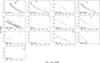 |
Fig. 1 Color-magnitude diagrams with Gaia DR3 photometric data (G vs. GBP – GRP) for the subset of clusters presented in this study for the first time as part of the SPA project. Red points indicate the member stars observed by SPA. |
3 Spectroscopic analysis
We first corrected the spectra for radial velocity (RV) and performed continuum normalization using the iSpec tool (Blanco-Cuaresma et al. 2014). The continuum normalization was performed using a spline function with 60 splines of quadratic order. A table providing an overview of the properties of our giant stars in 14 OCs is available online (see Data availability for more details). For the remaining sample, we refer to Casali et al. (2020a); Zhang et al. (2021, 2022); Alonso-Santiago et al. (2021). The table includes, for each star, Gaia DR3 (Gaia Collaboration 2023b) right ascension and declination, magnitudes, and RV, along with the total exposure time, the resulting signal-to-noise ratio (S/N), and the estimated RV and associated error obtained from iSpec. There is excellent agreement between the Gaia DR3 RV measurements and those of iSpec, with a mean difference of +0.08 km s−1. The comparison was performed after the exclusion of a few binary stars, either previously known or identified by us based on RV differences (see Sect. 4 for more details).
3.1 Stellar parameters
Spectroscopic parameters (Teff, log ɡ, metallicity [Fe/H]3, and microturbulent velocity, ξ) were obtained using the equivalent width (EW) method. The line list for Fe I and II transitions used in this work is based on Li & Ezzeddine (2023). These authors combine iron lines from the Gaia-ESO line list (Jofré et al. 2014; Heiter et al. 2015, 2021) and from the R-Process Alliance (RPA) survey (Hansen et al. 2018; Sakari et al. 2018; Ezzeddine et al. 2020; Holmbeck et al. 2020). In total, we used 165 Fe I and 20 Fe II lines4. The EWs were measured using the smhr tool5 (Casey 2014). Our method involved measuring the EW for a single reference star (#5 from IC 4756) using smhr. Subsequently, we calculated the EWs for the remainder of the sample using the reference star input masks with the stellardiff tool6. This code is specifically designed for differential analyses, allowing users to make assumptions about the local continuum around the spectral lines. This functionality helps minimize the effects of poor spectral normalization or unresolved features in the continuum. Additionally, we excluded any line with an EW greater than 200 mÅ and with an error exceeding 10 mÅ.
Initially, we employed the qoyllur-quipu (q2) LTE differential analysis code (Ramírez et al. 2014) on a test subsample of 14 OC stars, as routinely performed in previous works such as Casamiquela et al. (2017, 2019); Liu et al. (2016). The q2 tool is a Python package that utilizes MOOG (Sneden 1973) to calculate atmospheric parameters and abundances based on standard iron line excitation and ionization equilibrium techniques. The code works iteratively to adjust the parameters, aiming to minimize correlations with the excitation potential (χ) and the reduced equivalent width (REW), while also reducing the differences between the mean iron abundances derived from Fe I and Fe II lines. A notable strength of this code is its ability to perform line-by-line differential analysis, which offers a robust method for analyzing “twin” stars (as discussed, for example, in Meléndez et al. 2009). For the q2 method, we initially calculated differential parameters using the IC 4756 #5 as the reference for the entire sample. However, this approach proved inadequate due to the wide range of effective temperatures (Teff) and surface gravities (log ɡ) exhibited by our cluster giants. To address this, we established criteria for selecting multiple reference stars, ensuring that the differences between each star and its chosen reference satisfied the conditions of ΔTeff < 150 K and Δ log ɡ < 0.25. Ultimately, we identified four suitable reference stars (IC 4756 #4, #5, and #13 and UBC 170 #1). To choose these reference stars, we first ran the q2 method to compute the absolute parameters for all stars in the sample. We then used the absolute parameters of the reference stars to apply the q2 method again to derive the parameters for each subsample with their respective reference stars. However, recognizing the limitations of this method, which still resulted in a significant internal spread within each cluster, exceeding ≈0.20 dex (peak-to-valley) for giant stars, we opted to adopt an NLTE methodology and proceeded as follows.
We employed the code LOTUS (non-LTE Optimization Tool Utilized for the derivation of atmospheric Stellar parameters, Li & Ezzeddine 2023)7, which allows the derivation of atmospheric parameters (Teff, log ɡ, [Fe/H], and ξ) based on EW measurements of Fe I and Fe II lines. The LOTUS code performs interpolations of a generalized curve of growth (GCOG) from a grid of theoretical EWs in both LTE and NLTE, following the methodology outlined by Boeche & Grebel (2016). Stellar parameters are derived by minimizing the slopes of excitation and ionization equilibrium through an iterative global minimization process, with uncertainties in the atmospheric parameters estimated using a Markov chain Monte Carlo algorithm; further details are provided by Li & Ezzeddine 2023 (see their Sect. 2.5). Figure A.1 shows the corner plot of the posterior distribution of the stellar parameters and their uncertainties for IC 4756 #5. Users can select either LTE or NLTE modes within the code. When considering cool giants, adopting the NLTE approach over LTE-based analyses is crucial for accurately modeling their atmospheres. These stars have low surface gravities and densities, which prevent them from maintaining collisional equilibrium in their outer layers, causing a departure from LTE. NLTE effects arise from these imbalances, particularly in the ionization balance of elements such as iron, and can significantly impact the derived abundances and stellar parameters (see e.g., Bergemann et al. 2012; Lind et al. 2022, and references therein). Therefore, in this study, we chose to run LOTUS with NLTE corrections, applying the following input parameters to represent the stars in our sample: stellar type K (Teff ranging from 4000 K to 5200 K), giants (log ɡ between 0.5 dex and 3.0 dex) and metal rich ([Fe/H] from −0.5 to 0.5). We ran LOTUS on the 33 SPA OCs, comprising 95 giant stars. Table 2 reports the derived stellar parameters Teff, log ɡ, [Fe/H], and ξ for a subset of the sample. The full table is available at the CDS8. The uncertainties in [Fe/H] were calculated using  , where σ is the standard deviation of the Fe I lines given by LOTUS, and n is the total number of Fe I lines used in the analysis.
Figure 2 presents the stellar parameters [Fe/H], Teff, and log ɡ for clusters containing more than five giant stars. Within individual clusters, a noticeable trend emerges between metallicity and effective temperature, with cooler stars (those with Teff ≈ 4600 K) generally exhibiting lower metallicities. This trend also appears when considering surface gravity, as Teff and gravity are correlated in the sample. Indeed, removing the trend with Teff eliminates the correlation with log ɡ. This pattern is not novel and has been discussed in the literature (see, e.g., Casali et al. 2020a; Beeson et al. 2024).
Determining the underlying cause of these trends is complex and may involve several factors, including continuum displacement in cooler giants, the influence of blended features, the selection of line lists, and atomic parameters. Recently, Kos et al. (2025) reported abundance trends related to stellar parameters, particularly Teff, for OCs in GALAH DR4 (Buder et al. 2025). We refer to Kos et al. (2025) for a comprehensive discussion of the potential explanations for this trend. As also emphasized in Kos et al. (2025), atomic diffusion cannot explain the observed trend, as it operates under different parameters and evolutionary stages, leading to trends that differ from those observed.
Finally, an NLTE analysis reduces the discrepancies between warmer and cooler stars within the same clusters; however, it does not completely resolve the issue. This is clearly illustrated in Fig. 2, which compares LTE (lower panel) and NLTE parameters obtained using LOTUS. Given the amplitude trends calculated in Kos et al. (2025), our results are consistent with those of the GALAH stars for most elements. However, we observe larger internal variation for Sr and Y, which is primarily driven by a single cluster, Ruprecht 171, where a few cold stars contribute to the discrepancy.
In cases with a large number of stars per cluster, it may be appropriate to detrend these results, as performed by Kos et al. (2025). However, given the statistical limitation in our case, we present our abundance measurements as is, recognizing that this trend may introduce an internal precision limitation of less than ≈0.1 dex.
A direct and complete comparison of the LTE and NLTE results is beyond the scope of the present paper. We conclude this exercise by showing the differences between LTE and NLTE parameters in Fig. B.1. A clear positive trend is evident, indicating that stars with larger (and positive) LTE–NLTE temperature differences also display larger differences in surface gravity. This suggests that LTE analysis tends to overestimate both Teff and log ɡ, and that NLTE analysis mitigates these biases, yielding more consistent parameters across different stellar types.
Stellar parameters obtained with LOTUS for the 95 stars presented in this work.
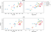 |
Fig. 2 Atmospheric parameters [Fe/H], Teff, and log ɡ obtained with LOTUS for clusters containing more than five stars. The first row presents the NLTE results, while the second row shows the LTE results. |
NLTE chemical abundances derived with TSFitPy for the 95 stars presented in this work.
3.2 Elemental abundances
To derive elemental abundances for species other than iron using NLTE grids in real-time (rather than through posterior corrections), only two spectral codes are currently available to our knowledge: the Python version of Spectroscopy Made Easy (SME; see Piskunov & Valenti 2017), pySME, developed by Wehrhahn et al. (2023), and the Python wrapper TSFitPy for Turbospectrum version 20 (Plez 2012), as described in Gerber et al. (2023) and Storm & Bergemann (2023). Our chosen strategy was to adopt the third option, TSFitPy, which allows the computation of synthetic spectra while incorporating NLTE corrections. The tool employs the Nelder–Mead algorithm to fit the normalized synthetic stellar spectra generated by Turbospectrum, minimizing the χ2 value in the process. The code offers access to two grids of stellar model atmospheres: the 1D line-blanketed hydrostatic MARCS models (Gustafsson et al. 2008) and average 3D Stagger models (Magic et al. 2013a,b). In this study, we adopted the 1D MARCS stellar grid.
We determined NLTE abundances for 11 chemical elements: Mg, Si, Ti, Na, Al, Mn, Co, Ni, Sr, Y, and Eu. In principle, a few more elements could have been included; however, the Ca lines were saturated and the Ba abundances appeared unrealistically high, preventing reliable measurements. The line list was constructed through a careful selection of isolated, unblended, and sufficiently strong lines within our spectral range9. Most lines originate from the Gaia-ESO Survey line list, with Sr I 4607 Å supplemented from the VALD database10. For Eu, only the 6645 Å line was used, as the strong resonance line at 4129 Å is blended at the metallicity of our sample stars. We have included hyperfine splitting when necessary (Mn, Co, and Eu lines).
The abundances were calculated as the average of the values derived for each line. The associated uncertainties were computed using  , where σ is the standard deviation and n is the number of stars per cluster. For the cases with only one line used, we adopted an uncertainty of 0.05 dex, as it is the typical mean abundance uncertainty in our sample (see Data availability for details on the sensitivities to stellar parameters table). The chemical abundances for a subset of stars are presented in Table 3; the full table is available at the CDS11.
We established our abundance scale by analyzing a solar spectrum, using a spectrum of Ganymede obtained with the HARPS spectrograph on the 3.6 m ESO telescope. The stellar parameters adopted for the Sun are: Teff=5771 K, log ɡ=4.44, logn(Fe)=7.52, and ξ=0.95 km s−1. The absolute solar abundances referenced by TSFitPy were sourced from Magg et al. (2022). The derived solar abundances are as follows: A(Mg) = 7.47 ± 0.10, A(Si) = 7.49 ± 0.04, A(Ti) = 5.00 ± 0.03, A(Na) = 6.24 ± 0.01, A(Al) = 6.44 ± 0.02, A(Mn) = 5.48 ± 0.02, A(Co) = 4.84 ± 0.07, A(Ni) = 6.20 ± 0.03, A(Sr) = 2.72 ± 0.10, and A(Y) = 1.98 ± 0.04. These values are consistent with those of Asplund et al. (2009) and Magg et al. (2022), within 2σ uncertainties, except for Y, which exhibits a deviation of 4σ. The Eu II line at 6645 Å was too weak in the solar spectrum to yield a reliable abundance measurement; therefore, no solar reference value could be determined. We adopted the value by Magg et al. (2022) of A(Eu)⊙=0.52. All other abundance ratios for our sample stars were computed using the solar abundances derived in this study.
We investigated correlations of [X/H] ratios with temperature and surface gravity considering the same OCs in Fig. 2; the results are presented in Fig. C.1. Within the uncertainties, we find no significant trends for Mg, Si, Ti, Na, and Al, as their behavior remains generally flat. However, for Mn, Co, Ni, Sr, Y, and Eu, the abundances show a slight increase with temperature (and log ɡ) along with notable scatter. Moreover, for Sr and Y we detect an upturn for Teff ≲ 4500 K.
Table 4 presents the mean abundances for the 33 OCs. The abundance of each cluster is computed as the average of its members, with the error given by  . For clusters with only one star, the uncertainty is taken as the standard deviation. Among our clusters, some interesting cases emerge, such as the super-solar metallicity OCs NGC 2509 ([Fe/H]=0.212 ± 0.01) and UBC 60 ([Fe/H]=0.227 ± 0.01). Conversely, Gulliver 51 and NGC 7044 exhibit the lowest values of our sample, with [Fe/H] ~ −0.2 dex.
Overall, we confirm that all OCs display a solar-scaled chemical composition with respect to the α elements (specifically Mg, Si, and Ti) and the iron peak elements Mn, Co, and Ni. While Na abundances are generally consistent with solar values within the uncertainties, they exhibit the well-known trend correlated with age. The neutron-capture elements Sr and Eu show a solar-scaled abundance pattern, whereas Y is slightly super-solar. Regarding the potential enhancement of s-process elements, which may be associated with magnetic activity at younger ages, we refer the reader to Spina et al. (2018), Baratella et al. (2021), Nordlander et al. (2024), and references therein.
4 Comparison with the literature
We used the OCs IC 4756, NGC 752, NGC 6991, and UBC 3, previously studied in the literature, for comparison with our results. Furthermore, as explained above, we include OCs previously analyzed by Casali et al. (2020a), D’Orazi et al. (2020), Zhang et al. (2021, 2022), and Alonso-Santiago et al. (2021). Several clusters studied by these authors have also been investigated in other independent studies. Here, we present a comprehensive comparison of all available data, integrating results from both our study and previous works to ensure consistency and identify discrepancies. In this comparison, we limited the dataset to high-resolution optical spectroscopy. The comparison results are summarized in Table D.1 and Fig. D.1.
For Teff and log ɡ, we compared our results with the literature on both cluster-by-cluster and star-by-star bases. For the clusters, we calculated the mean difference (this work, minus the literature) for each OC using stars in common. For the four OCs that are new to the SPA framework, we identified eight stars in common with the literature in IC 4756 (#0, #2, #4, #5, #7, #12, #13, and #14), three in NGC 752 (#3, #4, and #5), one in NGC 6991 (#1), and one in UBC 3 (#1) (see Table D.1 and Fig. D.1 for the references).
In general, there is good agreement in the results, considering the mean differences in Teff and log ɡ, as shown in Table D.1 and Fig. D.1. For [Fe/H] and [Mg/Fe], our results show an overall agreement, while [Si/Fe] is generally lower in this work. The abundance ratios [Ti/Fe], [Na/Fe], and [Al/Fe] exhibit some variations, typically up to 0.2 dex, with aluminum reaching −0.29 dex in NGC 752. Consistency is seen in [Mn/Fe], with a maximum difference of 0.3 dex in NGC 752. Good agreement is found for [Co/Fe] and [Ni/Fe], with differences up to 0.15 dex. For [Sr/Fe], with fewer clusters available for comparison, the maximum difference is −0.26 dex in UBC 3, while [Y/Fe] shows differences of around 0.2 dex. Similarly, [Eu/Fe] is available for a limited number of clusters, with a maximum difference of 0.18 dex. Notably, Jacobson et al. (2007) reported considerable variations for [Si/Fe], [Na/Fe], and [Al/Fe] in IC 4756 compared to our results. We note that the works presented here may use different solar scales, which could account for some of the observed differences.
Considering the previously published SPA OCs, Casali et al. (2020a) presented the spectral analysis of 15 stars in four OCs: Collinder 350, Gulliver 51, NGC 7044, and Ruprecht 171. The authors derived stellar parameters using both EW analysis with the Fast Automatic MOOG Analysis code (FAMA; Magrini et al. 2013) and a spectral fitting technique with ROTFIT (Frasca et al. 2006, 2019). One star in Gulliver 51 (#2), identified as a fast rotator, was excluded from our analysis. The Teff and log ɡ values show good agreement, as indicated by their mean differences (see Table D.1). More recently, Carbajo-Hijarrubia et al. (2024) also investigated Ruprecht 171, identifying three stars in common with our study (#5, #6, and #8), which show general agreement, with a mean difference of up to 220 K in temperature and 0.22 dex in [Fe/H].
Zhang et al. (2021) derived stellar parameters for 40 giant stars in 18 OCs using EW measurements. From this initial set, we excluded six binary stars (Gulliver 37 #1, NGC 2437 #6, NGC 2548 #4, NGC 2682 #3 and #4, and NGC 7082 #1 and #2) along with two stars (ASCC 11 #1 and NGC 2548 #4) that did not reach convergence with LOTUS. The results demonstrate good agreement in the mean differences of Teff and log ɡ, with the exceptions of COIN-Gaia 30 and Gulliver 18. Furthermore, some of these OCs have also been studied by other authors. We identified three stars in common in NGC 2548 (#1, #2, and #3), two stars in NGC 2682 (#1 and #2), and one star in Tombaugh 5 (#1); see Table D.1 for references. All display overall consistency in Teff and log ɡ compared to our results. Regarding abundance measurements, Table D.1 indicates agreement for [Fe/H] and [Mg/Fe], while our results generally show lower [Si/Fe] values. Differences in [Ti/Fe] are observed, typically up to 0.2 dex, with a maximum of 0.28 dex for NGC 2682. Additionally, [Na/Fe], [Al/Fe], [Mn/Fe], [Co/Fe], and [Ni/Fe] exhibit agreement within 0.2 dex. Finally, [Y/Fe] values in our study are generally higher compared to the literature, reaching 0.26 for NGC 2548. However, it should be noted that the literature generally reports LTE results.
Finally, Alonso-Santiago et al. (2021) analyzed 46 stars (both dwarfs and giants) in the OC Stock 2, determining stellar atmospheric parameters using ROTFIT and abundances using SYNTHE alongside an optimization tool. In our analysis, we have ten stars in common with Alonso-Santiago et al. (2021), although we excluded two binary stars (Stock 2 g3 and g5) from our sample. Additionally, as noted by Alonso-Santiago et al. (2021), Stock 2 was also studied by Reddy & Lambert (2019), and we have two stars in common with their analysis (#4 and #9). Overall, the results are in fair agreement.
Figure 3 presents the smoothed distribution of the differences in Teff and log ɡ for stars in common between this work and previous SPA studies. The distributions of ΔTeff and Δ log ɡ reveal significant spreads, particularly for Zhang et al. (2021) and Alonso-Santiago et al. (2021), which appear broader than those of Casali et al. (2020a) (ROTFIT and FAMA). Notably, however, the majority of stars exhibit differences concentrated around zero, indicating reasonable overall agreement between the results. The significant spreads in these distributions are primarily driven by a small subset of outlier stars. The mean values further suggest that LOTUS tends to yield lower Teff and log ɡ values compared to previous SPA results, as indicated by the leftward peaks in the distributions.
Figure 4 presents a comparative analysis of our results alongside previous SPA studies, focusing exclusively on SPA as it uses the same spectral data but employs different methodologies for calculating abundances. Notably, Zhang et al. (2022) applied NLTE corrections specifically to Na and Al, whereas Casali et al. (2020a) addressed NLTE effects for Fe but considered them negligible. Overall, we identify 19 SPA OCs in common for this comparison. Each line in the figure represents a distinct abundance, with our focus limited to [Fe/H], α, and odd-Z elements. The comparison emphasizes several key points: (i) differences in [Fe/H] values are generally close to 0.0 dex, indicating strong consistency, except in the case of NGC 2509; (ii) the [Mg/Fe] ratio shows greater variation, with a few clusters deviating by approximately ±0.2 dex; (iii) [Si/Fe] results are slightly lower in the present analysis, particularly for Alessi Teutsch 11, Gulliver 18, Gulliver 24, and UPK 219; (iv) differences in [Ti/Fe] are evident, with a maximum value reaching around ±0.15 dex; (v) [Na/Fe] exhibits substantial discrepancies, approaching ± 0.2 dex; (vi) [Al/Fe] exhibits similar trends to [Na/Fe], with variations present but generally less pronounced than for Na. Overall, this comparison demonstrates that, despite some variations, our results align well with previous studies for most elements. The observed differences in the comparison can primarily be attributed to three factors: the use of different line lists, variations in spectral analysis methodologies, and the adoption of NLTE abundances instead of LTE or a posteriori NLTE corrections. The methods employed in this study have resulted in reduced star-to-star scatter within each cluster, thereby providing higher internal precision.
Mean cluster abundance ratios.
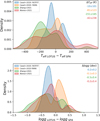 |
Fig. 3 Distribution of ΔTeff and Δ log ɡ comparing LOTUS results to those from previous SPA studies. The histograms were smoothed. The colors indicate the different authors. Mean differences and standard deviations are displayed in each panel. |
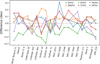 |
Fig. 4 Comparison between our results for Fe, α, and odd-z element abundances and those from previous SPA studies for each OC. The lines represent different elements. |
5 Galactic trends
We derived abundances for Fe and 11 chemical elements that are synthesized in different nucleosynthesis sites, including Type II and Type Ia supernovae (SNe) and asymptotic giant branch (AGB) stars, each contributing to the interstellar medium at different rates (see, e.g., Kobayashi et al. 2020; see also Romano et al. 2010, where uncertainties due to imperfect knowledge of stellar yields are discussed). More generally, studying how abundances change over time and across the Galactic disk is crucial to understanding the channels of element production and the various processes that have shaped the history of the Milky Way (Molero et al. 2023). In this context, OCs present a favorable option as they are distributed throughout the Galactic disk and encompass a wide range of ages that reflects a significant fraction of the lifespan of the thin disk. Furthermore, it is possible to characterize the chemistry of an OC using a small subset of its members.
We explored abundance trends in the Galactic disk using the mean abundances for the 33 OCs, combined with ages from Cantat-Gaudin et al. (2020). Our sample does not cover a large range in RGC. Most of our clusters are within about 1 kpc of the Sun (see Table 1) and are located farther away from the Galactic center than the Sun, reflecting the fact that we observed from the northern hemisphere. Conversely, our sample covers a broad range of age, from approximately 40 Myr to about 4 Gyr. We therefore chose to concentrate on the possible variations and evolution of abundances with age.
We included the OC sample from Spina et al. (2021) for visual comparison only, focusing specifically on the NLTE abundances reported in GALAH DR3 (Buder et al. 2021). Since our analysis is centered on NLTE abundances, we excluded comparisons with clusters from the Gaia-ESO survey (see, e.g., Magrini et al. 2023). Instead, Mg and Na from APOGEE DR17 were compared, as these elements were derived using NLTE corrections. They were included using the sample from Myers et al. (2022). Although Spina et al. standardized data from APOGEE and GALAH, our calculations of mean abundances are based exclusively on GALAH. The ages presented in the GALAH and APOGEE OC compilations are taken from Cantat-Gaudin et al. (2020). Our discussion encompasses a total of 63 OCs from the original sample reported by Spina et al. (2021)12, as well as an additional 84 OCs for Mg and 64 OCs for Na from Myers et al. (2022). The GALAH and APOGEE OCs are represented by gray symbols in Figs. 5, 6, and 7.
The elements shown in the diagrams can be divided into categories: α elements (Mg, Si, and Ti), iron-peak elements (Mn, Co, and Ni), odd-Z elements (Na and Al), and neutron-capture elements (Sr, Y, and Eu). Overall, our findings are consistent with the distribution observed in GALAH, except for the [Sr/Fe] ratio; however, our abundance ratios exhibit notably less scatter (see Fig. 5 and details in Sect. 5.4).
Regarding the age dependence, Fig. 6 illustrates the trend of [Fe/H] with age. As anticipated, there is no significant trend in OC metallicity relative to age, as the slope of the [Fe/H] versus age data is negligible. This supports the formation locus of a cluster as a more important factor for its chemical composition than age, suggesting a lack of an age-metallicity relationship. However, it must be noted that only a mild evolution is expected over the last 4.5 Gyr in the solar neighborhood. It is important to mention that when focusing on very young ages, most (though not all) of the clusters show slightly subsolar iron abundances (Kos et al. 2021; Alonso-Santiago et al. 2024). This observation appears to challenge the conventional model of Galactic chemical evolution, unless there has been a recent inflow of metal-poor material (see, e.g., Spitoni et al. 2023; Palla et al. 2024). This situation is atypical, and we would anticipate different behavior based on modeling predictions. However, magnetic activity may indeed be influencing the results (Spina et al. 2020; Baratella et al. 2021).
For each of the [X/Fe] ratios, we performed a linear fit of the abundance distributions versus age (shown in Fig. 7 as a thick blue line). The corresponding slopes and their uncertainties are given in Table 5, alongside the values for the SPA sample of Zhang et al. (2022) (18 OCs) and the OCCASO and OCCAM projects (Carbajo-Hijarrubia et al. 2024; Myers et al. 2022), which include 26 and 84 OCs, respectively. Since Myers et al. (2022) did not provide slopes for [X/Fe] versus age, we derived these values. The slopes obtained in this work are compatible within the uncertainties with those used for comparison. For Ti, Mn, and Ni, our slopes (0.039 ± 0.011, 0.040 ± 0.016, and 0.059 ± 0.018, respectively) are steeper than those from other studies, which range from 0.002 to 0.012 for Ti, −0.008 to 0.003 for Mn, and 0.010 to 0.026 for Ni. In OCCAM, a positive slope is found for Na (0.004 ± 0.009), whereas this work (−0.021 ± 0.012), the previous SPA study, and OCCASO all agree on negative slopes. Yttrium exhibits a shallower slope (−0.009 ± 0.013) in this work compared to OCCASO (−0.022 ± 0.012). No comparison is provided for Eu, as none of the references report a corresponding slope.
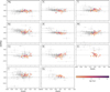 |
Fig. 5 Abundance ratios [X/Fe] as a function of [Fe/H]. The gray diamonds represent the OCs compilation from GALAH. Our results are color-coded according to the age. |
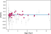 |
Fig. 6 Mean [Fe/H] per cluster as a function of age. The red points represent our sample of 33 OCs, while the gray diamonds correspond to clusters from GALAH. |
Slopes of [X/Fe] versus age and their associated uncertainties.
5.1 α elements
The α elements are primarily produced by core-collapse super-novae (CCSNe), which mark the final stage of the most massive stars (M ≥ 10 M⊙). Since these massive stars have short lifetimes (≤10−2 Gyr), they quickly enrich the interstellar medium relative to Fe, which is mainly produced on longer timescales through Type IA SNe (SNe Ia). In Fig. 5, Mg, Si and Ti show a relatively flat behavior with increasing metallicity, consistent with observations from GALAH OCs; Mg is also consistent with OCCAM OCs. Figure 7 illustrates a decrease in the abundance ratios of Mg, Si, and Ti with younger ages. This trend mirrors observations made for nearby solar twins (Nissen 2015; Spina et al. 2016; Casali et al. 2020b) and field stars (see, e.g., Buder et al. 2019; Delgado Mena et al. 2019; Hayden et al. 2022). Such behavior is anticipated in the Galactic disk, which initially formed from gas that was pre-enriched with α elements, followed by additional enrichment from subsequent generations of stars. The observed decline in [α/Fe] ratios with younger ages is consistent with predictions from Galactic chemical evolution models. In these models, successive generations of stars contribute significantly to α element enrichment through CCSNe, while the delayed contributions from SNe Ia increasingly dilute the ejecta from CCSNe as time progresses.
5.2 Odd-z elements
Sodium and aluminum are primarily produced by CCSNe, but are also produced during the AGB phase (see Smiljanic et al. (2016)). In AGB models, Na production is notably affected by metallicity, exhibiting secondary behavior whereby stars with higher metallicities tend to have larger Na abundances. Figure 5 displays a generally flat trend for sodium in our sample, despite some scatter. While a distinct declining trend is observed in the GALAH OCs, which span a wider range of metallicities compared to our sample, we must acknowledge the limitations posed by the smaller size of the SPA sample. This limitation introduces uncertainty regarding the interpretation of our findings, especially concerning the flatness and observed upward trend in [Na/Fe] for [Fe/H] > 0, which may be compatible with the GALAH distribution. This observation is consistent with recent findings by Owusu et al. (2024) and aligns with previous studies by, for example, Adibekyan et al. (2012); Nissen et al. (2020).
In contrast to Na, the [Al/Fe] trends are more closely associated with those of the α elements, likely due to their shared nucleosynthetic origins in massive stars (the AGB contribution to [Al/Fe] should be marginal within this metallicity range).
Figure 7 reveals several age-dependent trends, with Na decreasing and Al showing a mild increase as age progresses. The correlation between the behavior of Al and the α elements over time has also been observed in solar twins (Casali et al. 2020b) and field stars (Delgado Mena et al. 2019). The observed trend of decreasing [Na/Fe] with age is consistent with previous findings, for example, by Smiljanic et al. (2016, 2018). They report an increase in the surface Na abundance for red giants belonging to OCs with turnoff mass larger than approximately 2 M⊙ (i.e., younger than about 1 Gyr) and for Cepheids. The authors attribute this to evolutionary mixing processes; for these masses, additional Na is brought to the star surface at the first dredge-up, as confirmed by predictions from stellar evolutionary models (see, e.g., Lagarde et al. 2012; Ventura et al. 2013).
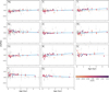 |
Fig. 7 Abundance ratios [X/Fe] as a function of age. The gray diamonds represent the OC compilation from GALAH, while the gray squares represent the OCs from OCCAM. Our results are color-coded according to [Fe/H]. |
5.3 Iron-peak elements
Type Ia SNe, resulting from white dwarf stars in interacting binary systems (Whelan & Iben 1973; Iben & Tutukov 1984), are the primary source of iron-peak elements (Kobayashi et al. 2011, 2020; Nomoto & Leung 2018). Both CCSNe and SNe Ia contribute to the nucleosynthesis of iron-group elements, including manganese. For metallicities of [Fe/H] ≲ – 1, CCSNe dominate Mn production in the solar neighborhood. However, the transition point at which SNe Ia begin to dominate varies across the Galactic disk: it occurs at lower [Fe/H] in the inner disk, where chemical evolution proceeds more rapidly, and at higher [Fe/H] in the outer disk, which evolves more slowly (Seitenzahl et al. 2013). Despite a general consensus on the qualitative roles of CCSNe and SNe Ia in producing Mn and Fe, the quantitative contributions remain uncertain. Consequently, the observed evolution of the [Mn/Fe] ratio with metallicity across the Galaxy is still not fully understood. Eitner et al. (2020) demonstrated that after accounting for NLTE corrections, the [Mn/Fe] ratio remains solar across all metallicities, from approximately [Fe/H] ≈ −4 to 0. Our sample enables us to explore the chemical evolution of Mn at super-solar metallicities. As shown in Fig. 5, we observe an increasing trend in [Mn/Fe] ratios with rising metallicity.
The [Co/Fe] ratios seem to follow a relatively flat trend, in agreement with previous studies for thin disk stars (e.g., Reddy et al. 2003, 2006). Conversely, we detect a mild decreasing trend of [Ni/Fe] for [Fe/H] < 0, although consistent with a solar-scaled pattern within uncertainties (see, e.g., Eitner et al. 2023); this is not seen in the GALAH sample.
Positive trends between Mn, Co, and Ni and age are observed in Fig. 7. The production of Ni is primarily attributed to SNe Ia, and a positive slope is not expected. This behavior is consistent with findings presented by Spina et al. (2021). The same trend is present in OCs studied by Carbajo-Hijarrubia et al. (2024), but not in the previous OCCASO studies. Recent 3D NLTE studies suggest that [Ni/Fe] may increase at lower metallicities due to NLTE effects (Storm et al. 2025), which could contribute to the trend in the metallicity regime covered by our sample. Manganese and Co display a mild increase with age, consistent with the delayed contributions from SNe Ia and the metallicity dependence of their yields. In the case of Mn, it is important to highlight that Galactic chemical evolution models fail to align with the NLTE abundances reported by Eitner et al. (2020), unless a threefold increase in the Mn yields from CCSNe is assumed. This is clearly illustrated in the work of Palla (2021) (see their Fig. 13), which also demonstrates that Mn can serve as an effective tool to differentiate between various SNe Ia yields, especially when precise measurements for metal-rich stars, such as those in this study, are available.
5.4 Neutron-capture elements
Elements heavier than iron are primarily formed through neutron-capture processes, with only a few proton-rich nuclei formed by photodisintegration. Two primary neutron-capture mechanisms have been identified in nature: the slow (s) and rapid (r) processes. These processes occur at opposite ends of the neutron density range, with the s-process occurring at lower densities and the r-process at extremely high densities. They are characterized by neutron-capture timescales that are slower or faster, respectively, than the beta-decay timescale of unstable nuclei. Together, these processes account for the majority of the abundances of elements heavier than iron in the Solar System (see recent reviews by Cowan et al. 2021 and Lugaro et al. 2023). For the s-process, the elements are predominantly produced in AGB stars (via the 13C(α,n)16O neutron source) or massive stars (via the 22Ne(α, n)25Mg. For the r-process, the main production channel remains under debate (compact mergers, special CCSNe; see, e.g., Cowan et al. 2021).
We inferred elemental abundances for the s-process elements yttrium and strontium, while barium lines were heavily saturated and susceptible to significant uncertainties. For this reason, we do not publish Ba abundances (see also the discussions in Baratella et al. 2021; Nordlander et al. 2024). In our targets, as well as in the GALAH sample, most young clusters exhibit super-solar [Y/Fe] ratios. This observation, previously noted in (young) OCs (Magrini et al. 2018; Baratella et al. 2021), is not unexpected. However, whether this enhancement is genuine is strongly debated in the literature (D’Orazi et al. 2022). Although Sr and Y belong to the first peak of the s-process and share similar nucleosynthetic origins, they exhibit different behaviors in our analysis. In particular, Sr demonstrates a flatter distribution, with the majority of clusters showing abundances consistent with solar levels. In contrast, the GALAH OCs exhibit exceptionally high super-solar abundances, exceeding 0.5 dex. However, these values were inferred using the neutral Sr line at 6550 Å, which is known to be blended (see also the discussion in the GALAH DR3 paper; Buder et al. 2021). Such values are inconsistent with any chemical evolution models. Therefore, we urge caution when interpreting these results, as they are subject to significant uncertainties. Europium abundances were also determined to trace the r-process contribution. Our findings indicate that europium abundances are consistent with solar-scaled patterns, aligning with observations from the GALAH sample, although GALAH data display a larger scatter. We find a slight positive slope with age, although not very significant. Delgado Mena et al. (2019) report a trend in the opposite direction (see their Fig. 7). However, this difference arises due to the inclusion of stars older than those in our sample; when restricting to a maximum age of 4 Gyr, their distribution also becomes nearly flat.
The interplay between the abundances of s-process elements and those of elements with opposite behaviors, such as the α elements, enhances their correlation with stellar age. This relationship has been highlighted, for instance, by Nissen (2015); Spina et al. (2016, 2018); Delgado Mena et al. (2019), who identified the [Y/Mg] ratio (among others) as a reliable chronometer for Galactic evolution. However, empirical relationships between neutron-capture elements and α elements are not consistent across the Galactic disk. Recent studies (see, e.g., Feltzing et al. 2017; Casali et al. 2020b; Viscasillas Vázquez et al. 2022) show that these relationships vary depending on metallicity and spatial location within the disk. This variation is significant, particularly given the presence of a metallicity gradient across the disk, especially in the inner region, extending to 12–14 kpc (see, e.g., Donor et al. 2020). To accurately calibrate these empirical relations, samples with precise age determinations are essential, and OCs represent one of the optimal choices within the high-metallicity regime (with [Fe/H] ranging from approximately −0.5 to 0.5 dex).
Figure 8 presents the [Y/Mg] ratios plotted against the ages of the OCs analyzed in this study. Our analysis reveals a nearly flat trend in [Y/Mg] versus age for clusters ranging from 100 Myr to approximately 1 Gyr, irrespective of the clusters’ metallicities or their positions within the Galaxy (although we acknowledge that our data cover a limited range). The youngest cluster in our sample, Gulliver 18, with an age of approximately 40 Myr, displays the highest [Y/Mg] ratios, with [Y/Fe] ratios three times greater than the solar value. In contrast, M 67, the oldest cluster in our sample, exhibits the lowest [Y/Mg] ratio. Notably, the ratios for other clusters within this range remain consistently flat with age, indicating that [Y/Mg] ratios may not be effective for dating the majority of OCs.
6 Summary
In this work, we examined 33 OCs observed by the SPA project, comprising a total of 95 giant stars with high-resolution HARPS-N spectra. Within the SPA framework, we chemically characterized 13 OCs and reanalyzed 20 previously studied clusters, creating a homogeneous and expanded sample. We presented NLTE atmospheric parameters derived using LOTUS through the equivalent width method and chemical abundances obtained via spectral synthesis with TSFitPy, covering ten elements from different nucleosynthesis groups.
Comparison of our results with those from the literature reveals good agreement. We explored Galactic trends in abundance ratios [X/Fe] as a function of metallicity and age. For comparison, we used the OCs studied by Spina et al. (2021), but with mean abundances derived exclusively from GALAH DR3 original data, and the OCs from the OCCAM survey analyzed by Myers et al. (2022). In general, our results follow similar trends to those observed in GALAH and APOGEE.
Regarding age trends, the α elements, such as Mg, Si, and Ti, show increasing trends with age. For the odd-Z elements, Na exhibits a decrease with age, while Al aligns more closely with the trends observed for α elements. The iron-peak elements, Mn, Co, and Ni, display a positive correlation with age. Neutron-capture Y and Eu shows a decreasing trend with age. These trends are consistent with expectations from Galactic chemical evolution models including the outcomes of nucleosynthesis processes in stars, except for Ni, and agree with previous studies.
In summary, this work adds nine additional OCs with full chemical characterization and explores age trends in elemental abundances, showing positive slopes for Mg, Si, Ti, Al, Mn, Co, and Ni and negative slopes for Na and Y. These results illustrate the important role of OCs as valuable tracers of Galactic chemical evolution, reinforcing that NLTE corrections are critical for accurate determinations of stellar parameters and abundances.
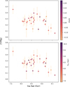 |
Fig. 8 [Y/Mg] as a function of age. The OCs from this work are color-coded by [Fe/H] in the top panel and by RGC in the bottom panel. |
Data availability
Full tables 2 and 3 are available at the CDS via https://cdsarc.cds.unistra.fr/viz-bin/cat/J/A+A/701/A289. Additionally, the following tables are available online at zenodo.org/records/15851389: (1) properties of the stars in the new OCs within the SPA project; (2) the iron line list; (3) the line list for TSFitPy spectral synthesis; (4) the abundance sensitivities; (5) the OCs selected from Spina et al. (2021) with mean abundances exclusively from GALAH DR3.
Acknowledgements
This research used the facilities of the Italian Center for Astronomical Archive (IA2) operated by INAF at the Astronomical Observatory of Trieste. This work has made use of data from the European Space Agency (ESA) mission Gaia (https://www.cosmos.esa.int/gaia), processed by the Gaia Data Processing and Analysis Consortium (DPAC, https://www.cosmos.esa.int/web/gaia/dpac/consortium). Funding for the DPAC has been provided by national institutions, in particular the institutions participating in the Gaia Multilateral Agreement. This research has made use of the VizieR catalog access tool, CDS, Strasbourg, France (DOI : 10.26093/cds/vizier). The original description of the VizieR service was published in 2000, A&AS 143, 23. Use of the NASA’s Astrophysical Data System and TOPCAT (Taylor 2005) are also acknowledged. We acknowledge funding from INAF MiniGrant 2022 (High resolution spectroscopy of open clusters) and the INAF grant Open Clusters and stellar structures in the local Galactic disk (ref. Antonella Vallenari) (CRA 1.05.23.05.19).
Appendix A LOTUS Markov-Chain Monte Carlo corner plot
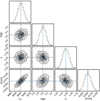 |
Fig. A.1 Marginalized posterior distributions of the stellar parameters for IC 4756 star #5, with the blue intersecting lines indicating the optimized parameters obtain by LOTUS. |
Appendix B Comparison of LTE and NLTE atmospheric parameters
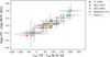 |
Fig. B.1 Differences between LTE and NLTE atmospheric parameters obtained with LOTUS for stars in five open clusters. |
Appendix C Abundance trends
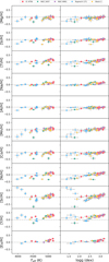 |
Fig. C.1 Abundances [X/H] as a function of Teff (first column) and log ɡ (second column). Each symbol represent a different open cluster. |
Appendix D Comparison with the literature
This table summarizes the comparison with the literature. For Teff and log ɡ we computed the mean differences (this work – literature) for each OC using the stars in common (N) and the error is the standard deviation. For metallicity and element abundances, we determined the differences by computing the mean cluster abundances derived in this work minus the same from the literature.
Differences of the atmospheric parameters and abundances for the OCs in common with the literature.
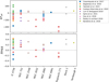 |
Fig. D.1 Comparison of atmospheric parameters for stars matched with the literature, showing star-by-star differences. |
References
- Adibekyan, V. Z., Sousa, S. G., Santos, N. C., et al. 2012, A&A, 545, A32 [NASA ADS] [CrossRef] [EDP Sciences] [Google Scholar]
- Alonso-Santiago, J., Frasca, A., Catanzaro, G., et al. 2021, A&A, 656, A149 [NASA ADS] [CrossRef] [EDP Sciences] [Google Scholar]
- Alonso-Santiago, J., Frasca, A., Bragaglia, A., et al. 2024, A&A, 691, A317 [NASA ADS] [CrossRef] [EDP Sciences] [Google Scholar]
- Asplund, M., Grevesse, N., Sauval, A. J., & Scott, P. 2009, ARA&A, 47, 481 [NASA ADS] [CrossRef] [Google Scholar]
- Bagdonas, V., Drazdauskas, A., Tautvaišiene, G., Smiljanic, R., & Chorniy, Y. 2018, A&A, 615, A165 [NASA ADS] [CrossRef] [EDP Sciences] [Google Scholar]
- Baratella, M., Carraro, G., D’Orazi, V., & Semenko, E. A. 2018, AJ, 156, 244 [NASA ADS] [CrossRef] [Google Scholar]
- Baratella, M., D’Orazi, V., Sheminova, V., et al. 2021, A&A, 653, A67 [NASA ADS] [CrossRef] [EDP Sciences] [Google Scholar]
- Beeson, K. L., Kos, J., de Grijs, R., et al. 2024, MNRAS, 529, 2483 [NASA ADS] [CrossRef] [Google Scholar]
- Bergemann, M., Lind, K., Collet, R., Magic, Z., & Asplund, M. 2012, MNRAS, 427, 27 [Google Scholar]
- Bhattacharya, S., Agarwal, M., Rao, K. K., & Vaidya, K. 2021, MNRAS, 505, 1607 [NASA ADS] [CrossRef] [Google Scholar]
- Blanco-Cuaresma, S., Soubiran, C., Heiter, U., & Jofré, P. 2014, A&A, 569, A111 [CrossRef] [EDP Sciences] [Google Scholar]
- Blanco-Cuaresma, S., Soubiran, C., Heiter, U., et al. 2015, A&A, 577, A47 [NASA ADS] [CrossRef] [EDP Sciences] [Google Scholar]
- Bijavara Seshashayana, S., Jönsson, H., D’Orazi, V., et al. 2024a, A&A, 683, A218 [NASA ADS] [CrossRef] [EDP Sciences] [Google Scholar]
- Bijavara Seshashayana, S., Jönsson, H., D’Orazi, V., et al. 2024b, A&A, 689, A120 [NASA ADS] [CrossRef] [EDP Sciences] [Google Scholar]
- Blanco-Cuaresma, S., & Fraix-Burnet, D. 2018, A&A, 618, A65 [NASA ADS] [CrossRef] [EDP Sciences] [Google Scholar]
- Böcek Topcu, G., Afsar, M., Schaeuble, M., & Sneden, C. 2015, MNRAS, 446, 3562 [Google Scholar]
- Boeche, C., & Grebel, E. K. 2016, A&A, 587, A2 [NASA ADS] [CrossRef] [EDP Sciences] [Google Scholar]
- Boesgaard, A. M., Lum, M. G., Chontos, A., & Deliyannis, C. P. 2022, ApJ, 927, 118 [NASA ADS] [CrossRef] [Google Scholar]
- Boffin, H. M. J., Jerabkova, T., Beccari, G., & Wang, L. 2022, MNRAS, 514, 3579 [NASA ADS] [CrossRef] [Google Scholar]
- Bossini, D., Vallenari, A., Bragaglia, A., et al. 2019, A&A, 623, A108 [NASA ADS] [CrossRef] [EDP Sciences] [Google Scholar]
- Bragaglia, A., & Tosi, M. 2006, AJ, 131, 1544 [Google Scholar]
- Buder, S., Lind, K., Ness, M. K., et al. 2019, A&A, 624, A19 [NASA ADS] [CrossRef] [EDP Sciences] [Google Scholar]
- Buder, S., Sharma, S., Kos, J., et al. 2021, MNRAS, 506, 150 [NASA ADS] [CrossRef] [Google Scholar]
- Buder, S., Kos, J., Wang, X. E., et al. 2025, PASA, 42, e051 [Google Scholar]
- Cantat-Gaudin, T., Vallenari, A., Sordo, R., et al. 2018, A&A, 615, A49 [NASA ADS] [CrossRef] [EDP Sciences] [Google Scholar]
- Cantat-Gaudin, T., Anders, F., Castro-Ginard, A., et al. 2020, A&A, 640, A1 [NASA ADS] [CrossRef] [EDP Sciences] [Google Scholar]
- Carbajo-Hijarrubia, J., Casamiquela, L., Carrera, R., et al. 2024, A&A, 687, A239 [NASA ADS] [CrossRef] [EDP Sciences] [Google Scholar]
- Carraro, G., Monaco, L., & Villanova, S. 2014, A&A, 568, A86 [NASA ADS] [CrossRef] [EDP Sciences] [Google Scholar]
- Carrera, R., & Pancino, E. 2011, A&A, 535, A30 [NASA ADS] [CrossRef] [EDP Sciences] [Google Scholar]
- Casali, G., Magrini, L., Frasca, A., et al. 2020a, A&A, 643, A12 [NASA ADS] [CrossRef] [EDP Sciences] [Google Scholar]
- Casali, G., Spina, L., Magrini, L., et al. 2020b, A&A, 639, A127 [NASA ADS] [CrossRef] [EDP Sciences] [Google Scholar]
- Casamiquela, L., Carrera, R., Blanco-Cuaresma, S., et al. 2017, MNRAS, 470, 4363 [NASA ADS] [CrossRef] [Google Scholar]
- Casamiquela, L., Blanco-Cuaresma, S., Carrera, R., et al. 2019, MNRAS, 490, 1821 [NASA ADS] [CrossRef] [Google Scholar]
- Casey, A. R. 2014, PhD thesis, Australian National University, Canberra [Google Scholar]
- Castro-Ginard, A., Jordi, C., Luri, X., et al. 2018, A&A, 618, A59 [NASA ADS] [CrossRef] [EDP Sciences] [Google Scholar]
- Castro-Ginard, A., Jordi, C., Luri, X., Cantat-Gaudin, T., & Balaguer-Núñez, L. 2019, A&A, 627, A35 [NASA ADS] [CrossRef] [EDP Sciences] [Google Scholar]
- Castro-Ginard, A., Jordi, C., Luri, X., et al. 2020, A&A, 635, A45 [NASA ADS] [CrossRef] [EDP Sciences] [Google Scholar]
- Cosentino, R., Lovis, C., Pepe, F., et al. 2012, SPIE Conf. Ser., 8446, 84461V [Google Scholar]
- Cowan, J. J., Sneden, C., Lawler, J. E., et al. 2021, Rev. Mod. Phys., 93, 015002 [Google Scholar]
- Cummings, J. D., Deliyannis, C. P., Maderak, R. M., & Steinhauer, A. 2017, AJ, 153, 128 [Google Scholar]
- Dalton, G., Trager, S., Abrams, D. C., et al. 2018, SPIE Conf. Ser., 10702, 107021B [Google Scholar]
- de Jong, R. S., Agertz, O., Berbel, A. A., et al. 2019, The Messenger, 175, 3 [NASA ADS] [Google Scholar]
- De Silva, G. M., Freeman, K. C., Bland-Hawthorn, J., et al. 2015, MNRAS, 449, 2604 [NASA ADS] [CrossRef] [Google Scholar]
- Delgado Mena, E., Moya, A., Adibekyan, V., et al. 2019, A&A, 624, A78 [NASA ADS] [CrossRef] [EDP Sciences] [Google Scholar]
- Donor, J., Frinchaboy, P. M., Cunha, K., et al. 2020, AJ, 159, 199 [NASA ADS] [CrossRef] [Google Scholar]
- D’Orazi, V., Oliva, E., Bragaglia, A., et al. 2020, A&A, 633, A38 [NASA ADS] [CrossRef] [EDP Sciences] [Google Scholar]
- D’Orazi, V., Baratella, M., Lugaro, M., Magrini, L., & Pignatari, M. 2022, Universe, 8, 110 [CrossRef] [Google Scholar]
- Eitner, P., Bergemann, M., Hansen, C. J., et al. 2020, A&A, 635, A38 [NASA ADS] [CrossRef] [EDP Sciences] [Google Scholar]
- Eitner, P., Bergemann, M., Ruiter, A. J., et al. 2023, A&A, 677, A151 [NASA ADS] [CrossRef] [EDP Sciences] [Google Scholar]
- Ezzeddine, R., Rasmussen, K., Frebel, A., et al. 2020, ApJ, 898, 150 [NASA ADS] [CrossRef] [Google Scholar]
- Fanelli, C., Origlia, L., Oliva, E., et al. 2022, A&A, 660, A7 [NASA ADS] [CrossRef] [EDP Sciences] [Google Scholar]
- Feltzing, S., Howes, L. M., McMillan, P. J., & Stonkute, E. 2017, MNRAS, 465, L109 [NASA ADS] [CrossRef] [Google Scholar]
- Frasca, A., Guillout, P., Marilli, E., et al. 2006, A&A, 454, 301 [NASA ADS] [CrossRef] [EDP Sciences] [Google Scholar]
- Frasca, A., Alonso-Santiago, J., Catanzaro, G., et al. 2019, A&A, 632, A16 [NASA ADS] [EDP Sciences] [Google Scholar]
- Friel, E. D., Jacobson, H. R., & Pilachowski, C. A. 2010, AJ, 139, 1942 [NASA ADS] [CrossRef] [Google Scholar]
- Frinchaboy, P. M., Thompson, B., Jackson, K. M., et al. 2013, ApJ, 777, L1 [NASA ADS] [CrossRef] [Google Scholar]
- Fu, X., Bragaglia, A., Liu, C., et al. 2022, A&A, 668, A4 [NASA ADS] [CrossRef] [EDP Sciences] [Google Scholar]
- Gaia Collaboration (Prusti, T., et al.) 2016, A&A, 595, A1 [NASA ADS] [CrossRef] [EDP Sciences] [Google Scholar]
- Gaia Collaboration (Recio-Blanco, A., et al.) 2023a, A&A, 674, A38 [CrossRef] [EDP Sciences] [Google Scholar]
- Gaia Collaboration (Vallenari, A., et al.) 2023b, A&A, 674, A1 [NASA ADS] [CrossRef] [EDP Sciences] [Google Scholar]
- Gao, X., Lind, K., Amarsi, A. M., et al. 2018, MNRAS, 481, 2666 [NASA ADS] [CrossRef] [Google Scholar]
- Gerber, J. M., Magg, E., Plez, B., et al. 2023, A&A, 669, A43 [NASA ADS] [CrossRef] [EDP Sciences] [Google Scholar]
- Gilmore, G., Randich, S., Asplund, M., et al. 2012, The Messenger, 147, 25 [NASA ADS] [Google Scholar]
- Gustafsson, B., Edvardsson, B., Eriksson, K., et al. 2008, A&A, 486, 951 [NASA ADS] [CrossRef] [EDP Sciences] [Google Scholar]
- Hansen, T. T., Holmbeck, E. M., Beers, T. C., et al. 2018, ApJ, 858, 92 [Google Scholar]
- Hao, C. J., Xu, Y., Wu, Z. Y., et al. 2022, A&A, 660, A4 [NASA ADS] [CrossRef] [EDP Sciences] [Google Scholar]
- Hayden, M. R., Sharma, S., Bland-Hawthorn, J., et al. 2022, MNRAS, 517, 5325 [NASA ADS] [CrossRef] [Google Scholar]
- Heiter, U., Jofré, P., Gustafsson, B., et al. 2015, A&A, 582, A49 [NASA ADS] [CrossRef] [EDP Sciences] [Google Scholar]
- Heiter, U., Lind, K., Bergemann, M., et al. 2021, A&A, 645, A106 [EDP Sciences] [Google Scholar]
- Holmbeck, E. M., Hansen, T. T., Beers, T. C., et al. 2020, ApJS, 249, 30 [NASA ADS] [CrossRef] [Google Scholar]
- Hunt, E. L., & Reffert, S. 2023, A&A, 673, A114 [NASA ADS] [CrossRef] [EDP Sciences] [Google Scholar]
- Iben, Jr., I., & Tutukov, A. V. 1984, ApJS, 54, 335 [NASA ADS] [CrossRef] [Google Scholar]
- Jacobson, H. R., Friel, E. D., & Pilachowski, C. A. 2007, AJ, 134, 1216 [NASA ADS] [CrossRef] [Google Scholar]
- Jacobson, H. R., Pilachowski, C. A., & Friel, E. D. 2011, AJ, 142, 59 [NASA ADS] [CrossRef] [Google Scholar]
- Janes, K. A. 1979, ApJS, 39, 135 [NASA ADS] [CrossRef] [Google Scholar]
- Jian, M., Fu, X., Matsunaga, N., et al. 2024, A&A, 687, A189 [NASA ADS] [CrossRef] [EDP Sciences] [Google Scholar]
- Jin, S., Trager, S. C., Dalton, G. B., et al. 2024, MNRAS, 530, 2688 [NASA ADS] [CrossRef] [Google Scholar]
- Jofré, P., Heiter, U., Soubiran, C., et al. 2014, A&A, 564, A133 [NASA ADS] [CrossRef] [EDP Sciences] [Google Scholar]
- Kobayashi, C., Karakas, A. I., & Umeda, H. 2011, MNRAS, 414, 3231 [Google Scholar]
- Kobayashi, C., Karakas, A. I., & Lugaro, M. 2020, ApJ, 900, 179 [Google Scholar]
- Kos, J. 2024, A&A, 691, A28 [NASA ADS] [CrossRef] [EDP Sciences] [Google Scholar]
- Kos, J., Bland-Hawthorn, J., Buder, S., et al. 2021, MNRAS, 506, 4232 [NASA ADS] [CrossRef] [Google Scholar]
- Kos, J., Buder, S., Beeson, K. L., et al. 2025, A&A, submitted [arXiv:2501.06140] [Google Scholar]
- Kounkel, M., & Covey, K. 2019, AJ, 158, 122 [Google Scholar]
- Lagarde, N., Decressin, T., Charbonnel, C., et al. 2012, A&A, 543, A108 [NASA ADS] [CrossRef] [EDP Sciences] [Google Scholar]
- Li, Y., & Ezzeddine, R. 2023, AJ, 165, 145 [NASA ADS] [CrossRef] [Google Scholar]
- Lind, K., Nordlander, T., Wehrhahn, A., et al. 2022, A&A, 665, A33 [NASA ADS] [CrossRef] [EDP Sciences] [Google Scholar]
- Liu, L., & Pang, X. 2019, ApJS, 245, 32 [NASA ADS] [CrossRef] [Google Scholar]
- Liu, F., Asplund, M., Yong, D., et al. 2016, MNRAS, 463, 696 [NASA ADS] [CrossRef] [Google Scholar]
- Lucatello, S., Bragaglia, A., Vallenari, A., et al. 2023, The Messenger, 190, 13 [NASA ADS] [Google Scholar]
- Lugaro, M., Pignatari, M., Reifarth, R., & Wiescher, M. 2023, Annu. Rev. Nucl. Part. Sci., 73, 315 [NASA ADS] [CrossRef] [Google Scholar]
- Lum, M. G., & Boesgaard, A. M. 2019, ApJ, 878, 99 [NASA ADS] [CrossRef] [Google Scholar]
- Magg, E., Bergemann, M., Serenelli, A., et al. 2022, A&A, 661, A140 [NASA ADS] [CrossRef] [EDP Sciences] [Google Scholar]
- Magic, Z., Collet, R., Asplund, M., et al. 2013a, A&A, 557, A26 [NASA ADS] [CrossRef] [EDP Sciences] [Google Scholar]
- Magic, Z., Collet, R., Hayek, W., & Asplund, M. 2013b, A&A, 560, A8 [NASA ADS] [CrossRef] [EDP Sciences] [Google Scholar]
- Magrini, L., Sestito, P., Randich, S., & Galli, D. 2009, A&A, 494, 95 [NASA ADS] [CrossRef] [EDP Sciences] [Google Scholar]
- Magrini, L., Randich, S., Friel, E., et al. 2013, A&A, 558, A38 [NASA ADS] [CrossRef] [EDP Sciences] [Google Scholar]
- Magrini, L., Spina, L., Randich, S., et al. 2018, A&A, 617, A106 [NASA ADS] [CrossRef] [EDP Sciences] [Google Scholar]
- Magrini, L., Viscasillas Vazquez, C., Spina, L., et al. 2023, A&A, 669, A119 [NASA ADS] [CrossRef] [EDP Sciences] [Google Scholar]
- Majewski, S. R., Schiavon, R. P., Frinchaboy, P. M., et al. 2017, AJ, 154, 94 [NASA ADS] [CrossRef] [Google Scholar]
- Meléndez, J., Asplund, M., Gustafsson, B., & Yong, D. 2009, ApJ, 704, L66 [Google Scholar]
- Molero, M., Magrini, L., Matteucci, F., et al. 2023, MNRAS, 523, 2974 [NASA ADS] [CrossRef] [Google Scholar]
- Monteiro, H., & Dias, W. S. 2019, MNRAS, 487, 2385 [Google Scholar]
- Myers, N., Donor, J., Spoo, T., et al. 2022, AJ, 164, 85 [NASA ADS] [CrossRef] [Google Scholar]
- Netopil, M., Paunzen, E., Heiter, U., & Soubiran, C. 2016, A&A, 585, A150 [NASA ADS] [CrossRef] [EDP Sciences] [Google Scholar]
- Nissen, P. E. 2015, A&A, 579, A52 [NASA ADS] [CrossRef] [EDP Sciences] [Google Scholar]
- Nissen, P. E., Christensen-Dalsgaard, J., Mosumgaard, J. R., et al. 2020, A&A, 640, A81 [NASA ADS] [CrossRef] [EDP Sciences] [Google Scholar]
- Nomoto, K., & Leung, S.-C. 2018, Space Sci. Rev., 214, 67 [NASA ADS] [CrossRef] [Google Scholar]
- Nordlander, T., Baratella, M., Spina, L., & D’Orazi, V. 2024, MNRAS, 535, 2863 [Google Scholar]
- Owusu, E. K., Buder, S., Ruiter, A. J., Seitenzahl, I. R., & Rodriguez-Segovia, N. 2024, PASA, 41, e092 [Google Scholar]
- Pace, G., Danziger, J., Carraro, G., et al. 2010, A&A, 515, A28 [NASA ADS] [CrossRef] [EDP Sciences] [Google Scholar]
- Pakhomov, Y. V., Antipova, L. I., Boyarchuk, A. A., et al. 2009, Astron. Rep., 53, 660 [NASA ADS] [CrossRef] [Google Scholar]
- Palla, M. 2021, MNRAS, 503, 3216 [Google Scholar]
- Palla, M., Magrini, L., Spitoni, E., et al. 2024, A&A, 690, A334 [NASA ADS] [CrossRef] [EDP Sciences] [Google Scholar]
- Pancino, E., Carrera, R., Rossetti, E., & Gallart, C. 2010, A&A, 511, A56 [NASA ADS] [CrossRef] [EDP Sciences] [Google Scholar]
- Piskunov, N., & Valenti, J. A. 2017, A&A, 597, A16 [NASA ADS] [CrossRef] [EDP Sciences] [Google Scholar]
- Plez, B. 2012, Turbospectrum: Code for spectral synthesis, Astrophysics Source Code Library [record ascl:1205.004] [Google Scholar]
- Ramirez, I., Meléndez, J., Bean, J., et al. 2014, A&A, 572, A48 [Google Scholar]
- Ramos, A. A., Holanda, N., Drake, N. A., et al. 2024, MNRAS, 527, 6211 [Google Scholar]
- Randich, S., Gilmore, G., & Gaia-ESO Consortium 2013, The Messenger, 154, 47 [NASA ADS] [Google Scholar]
- Randich, S., Gilmore, G., Magrini, L., et al. 2022, A&A, 666, A121 [NASA ADS] [CrossRef] [EDP Sciences] [Google Scholar]
- Ray, A. E., Frinchaboy, P. M., Donor, J., Chojnowski, S. D., & Melendez, M. 2022, AJ, 163, 195 [Google Scholar]
- Reddy, A. B. S., & Lambert, D. L. 2019, MNRAS, 485, 3623 [NASA ADS] [CrossRef] [Google Scholar]
- Reddy, B. E., Tomkin, J., Lambert, D. L., & Allende Prieto, C. 2003, MNRAS, 340, 304 [Google Scholar]
- Reddy, B. E., Lambert, D. L., & Allende Prieto, C. 2006, MNRAS, 367, 1329 [Google Scholar]
- Reddy, A. B. S., Giridhar, S., & Lambert, D. L. 2012, MNRAS, 419, 1350 [CrossRef] [Google Scholar]
- Romano, D., Karakas, A. I., Tosi, M., & Matteucci, F. 2010, A&A, 522, A32 [NASA ADS] [CrossRef] [EDP Sciences] [Google Scholar]
- Sakari, C. M., Placco, V. M., Farrell, E. M., et al. 2018, ApJ, 868, 110 [Google Scholar]
- Santos, N. C., Lovis, C., Pace, G., Melendez, J., & Naef, D. 2009, A&A, 493, 309 [NASA ADS] [CrossRef] [EDP Sciences] [Google Scholar]
- Seitenzahl, I. R., Cescutti, G., Röpke, F. K., Ruiter, A. J., & Pakmor, R. 2013, A&A, 559, L5 [NASA ADS] [CrossRef] [EDP Sciences] [Google Scholar]
- Seshashayana, S. B., Jönsson, H., D’Orazi, V., et al. 2024, A&A, 683, A218 [NASA ADS] [CrossRef] [EDP Sciences] [Google Scholar]
- Sestito, P., Randich, S., & Pallavicini, R. 2004, A&A, 426, 809 [NASA ADS] [CrossRef] [EDP Sciences] [Google Scholar]
- Sestito, P., Bragaglia, A., Randich, S., et al. 2008, A&A, 488, 943 [NASA ADS] [CrossRef] [EDP Sciences] [Google Scholar]
- Sim, G., Lee, S. H., Ann, H. B., & Kim, S. 2019, J. Korean Astron. Soc., 52, 145 [NASA ADS] [Google Scholar]
- Smiljanic, R., Gauderon, R., North, P., et al. 2009, A&A, 502, 267 [NASA ADS] [CrossRef] [EDP Sciences] [Google Scholar]
- Smiljanic, R., Romano, D., Bragaglia, A., et al. 2016, A&A, 589, A115 [NASA ADS] [CrossRef] [EDP Sciences] [Google Scholar]
- Smiljanic, R., Donati, P., Bragaglia, A., Lemasle, B., & Romano, D. 2018, A&A, 616, A112 [NASA ADS] [CrossRef] [EDP Sciences] [Google Scholar]
- Sneden, C. A. 1973, PhD thesis, University of Texas, Austin [Google Scholar]
- Spina, L., Meléndez, J., Karakas, A. I., et al. 2016, A&A, 593, A125 [NASA ADS] [CrossRef] [EDP Sciences] [Google Scholar]
- Spina, L., Meléndez, J., Karakas, A. I., et al. 2018, MNRAS, 474, 2580 [NASA ADS] [Google Scholar]
- Spina, L., Nordlander, T., Casey, A. R., et al. 2020, ApJ, 895, 52 [Google Scholar]
- Spina, L., Ting, Y. S., De Silva, G. M., et al. 2021, MNRAS, 503, 3279 [CrossRef] [Google Scholar]
- Spitoni, E., Recio-Blanco, A., de Laverny, P., et al. 2023, A&A, 670, A109 [NASA ADS] [CrossRef] [EDP Sciences] [Google Scholar]
- Storm, N., & Bergemann, M. 2023, MNRAS, 525, 3718 [NASA ADS] [CrossRef] [Google Scholar]
- Storm, N., Bergemann, M., Eitner, P., et al. 2025, MNRAS, 538, 3284 [Google Scholar]
- Sun, Q., Deliyannis, C. P., Steinhauer, A., Twarog, B. A., & Anthony-Twarog, B. J. 2020, AJ, 159, 220 [NASA ADS] [CrossRef] [Google Scholar]
- Tautvaišiene, G., Edvardsson, B., Tuominen, I., & Ilyin, I. 2000, A&A, 360, 499 [NASA ADS] [Google Scholar]
- Taylor, M. B. 2005, in Astronomical Society of the Pacific Conference Series, 347, Astronomical Data Analysis Software and Systems XIV, eds. P. Shopbell, M. Britton, & R. Ebert, 29 [NASA ADS] [Google Scholar]
- Ting, Y.-S., De Silva, G. M., Freeman, K. C., & Parker, S. J. 2012, MNRAS, 427, 882 [Google Scholar]
- Tsantaki, M., Delgado-Mena, E., Bossini, D., et al. 2023, A&A, 674, A157 [NASA ADS] [CrossRef] [EDP Sciences] [Google Scholar]
- Vejar, G., Schuler, S. C., & Stassun, K. G. 2021, ApJ, 919, 100 [NASA ADS] [CrossRef] [Google Scholar]
- Ventura, P., Di Criscienzo, M., Carini, R., & D’Antona, F. 2013, MNRAS, 431, 3642 [Google Scholar]
- Vernekar, N., Lucatello, S., Bragaglia, A., et al. 2024, A&A, 684, A85 [NASA ADS] [CrossRef] [EDP Sciences] [Google Scholar]
- Viscasillas Vázquez, C., Magrini, L., Casali, G., et al. 2022, A&A, 660, A135 [NASA ADS] [CrossRef] [EDP Sciences] [Google Scholar]
- Viscasillas Vázquez, C., Magrini, L., Spina, L., et al. 2023, A&A, 679, A122 [NASA ADS] [CrossRef] [EDP Sciences] [Google Scholar]
- Wehrhahn, A., Piskunov, N., & Ryabchikova, T. 2023, A&A, 671, A171 [NASA ADS] [CrossRef] [EDP Sciences] [Google Scholar]
- Whelan, J., & Iben, Jr., I. 1973, ApJ, 186, 1007 [CrossRef] [Google Scholar]
- Yong, D., Carney, B. W., Teixera de Almeida, M. L., & Pohl, B. L. 2006, AJ, 131, 2256 [NASA ADS] [CrossRef] [Google Scholar]
- Zhang, R., Lucatello, S., Bragaglia, A., et al. 2021, A&A, 654, A77 [NASA ADS] [CrossRef] [EDP Sciences] [Google Scholar]
- Zhang, R., Lucatello, S., Bragaglia, A., et al. 2022, A&A, 667, A103 [NASA ADS] [CrossRef] [EDP Sciences] [Google Scholar]
- Zhao, G., Zhao, Y.-H., Chu, Y.-Q., Jing, Y.-P., & Deng, L.-C. 2012, Res. Astron. Astrophys., 12, 723 [NASA ADS] [CrossRef] [Google Scholar]
The cluster Collinder 350 is analyzed in both Casali et al. (2020a) and Zhang et al. (2021).
Some of the UBC and UPK clusters correspond to rediscoveries of previously known objects; see the cited studies for cross-matching with older catalogs.
We adopt the standard spectroscopic notation of ![Mathematical equation: $\left[ {{\rm{Fe/H}}} \right] = \log {{N{{\left( {Fe} \right)}_*}} \over {N{{\left( H \right)}_*}}} - \log {{N{{\left( {Fe} \right)}_ \odot }} \over {N{{\left( H \right)}_ \odot }}}$](/articles/aa/full_html/2025/09/aa54258-25/aa54258-25-eq4.png) .
.
The line list is available online (see Data availability for more details).
The complete line list is available online (see Data availability for more details).
The complete table is available online (see Data availability for more details).
All Tables
Summary of the clusters analyzed in this work, including their properties and the number of stars in each cluster (N).
NLTE chemical abundances derived with TSFitPy for the 95 stars presented in this work.
Differences of the atmospheric parameters and abundances for the OCs in common with the literature.
All Figures
|
Fig. 1 Color-magnitude diagrams with Gaia DR3 photometric data (G vs. GBP – GRP) for the subset of clusters presented in this study for the first time as part of the SPA project. Red points indicate the member stars observed by SPA. |
| In the text | |
|
Fig. 2 Atmospheric parameters [Fe/H], Teff, and log ɡ obtained with LOTUS for clusters containing more than five stars. The first row presents the NLTE results, while the second row shows the LTE results. |
| In the text | |
|
Fig. 3 Distribution of ΔTeff and Δ log ɡ comparing LOTUS results to those from previous SPA studies. The histograms were smoothed. The colors indicate the different authors. Mean differences and standard deviations are displayed in each panel. |
| In the text | |
|
Fig. 4 Comparison between our results for Fe, α, and odd-z element abundances and those from previous SPA studies for each OC. The lines represent different elements. |
| In the text | |
|
Fig. 5 Abundance ratios [X/Fe] as a function of [Fe/H]. The gray diamonds represent the OCs compilation from GALAH. Our results are color-coded according to the age. |
| In the text | |
|
Fig. 6 Mean [Fe/H] per cluster as a function of age. The red points represent our sample of 33 OCs, while the gray diamonds correspond to clusters from GALAH. |
| In the text | |
|
Fig. 7 Abundance ratios [X/Fe] as a function of age. The gray diamonds represent the OC compilation from GALAH, while the gray squares represent the OCs from OCCAM. Our results are color-coded according to [Fe/H]. |
| In the text | |
|
Fig. 8 [Y/Mg] as a function of age. The OCs from this work are color-coded by [Fe/H] in the top panel and by RGC in the bottom panel. |
| In the text | |
|
Fig. A.1 Marginalized posterior distributions of the stellar parameters for IC 4756 star #5, with the blue intersecting lines indicating the optimized parameters obtain by LOTUS. |
| In the text | |
|
Fig. B.1 Differences between LTE and NLTE atmospheric parameters obtained with LOTUS for stars in five open clusters. |
| In the text | |
|
Fig. C.1 Abundances [X/H] as a function of Teff (first column) and log ɡ (second column). Each symbol represent a different open cluster. |
| In the text | |
|
Fig. D.1 Comparison of atmospheric parameters for stars matched with the literature, showing star-by-star differences. |
| In the text | |
Current usage metrics show cumulative count of Article Views (full-text article views including HTML views, PDF and ePub downloads, according to the available data) and Abstracts Views on Vision4Press platform.
Data correspond to usage on the plateform after 2015. The current usage metrics is available 48-96 hours after online publication and is updated daily on week days.
Initial download of the metrics may take a while.