| Issue |
A&A
Volume 701, September 2025
|
|
|---|---|---|
| Article Number | A12 | |
| Number of page(s) | 25 | |
| Section | Extragalactic astronomy | |
| DOI | https://doi.org/10.1051/0004-6361/202554394 | |
| Published online | 01 September 2025 | |
Quantifying biases in orbit-superposition modelling with (non-)parametric kinematics
Department of Astrophysics, University of Vienna, Türkenschanzstrasse 17, A-1180 Vienna, Austria
⋆ Corresponding author: This email address is being protected from spambots. You need JavaScript enabled to view it.
Received:
6
March
2025
Accepted:
12
July
2025
Abstract
Context. Dynamical models enable the recovery of galaxy mass profiles, intrinsic shapes, and, in the case of Schwarzschild orbit-superposition methods, orbital structure. An accurate dynamical inference relies on the precise recovery of the line-of-sight velocity distribution from an integrated spectrum.
Aims. The main goal of this work is to evaluate the effect of different methods for recovering stellar kinematics from an integrated spectrum on the resulting orbit distribution and subsequent implications on the recovered mass and velocity anisotropy profiles.
Methods. We applied the commonly used penalised pixel fitting method pPXF on archival SAURON datacubes of NGC 4550 and NGC 2768, a well-studied counter-rotating and a regular-rotating elliptical galaxy, for a parametrised description of the stellar line-of-sight velocity distribution based on Gauss Hermite expansion. We also used Bayes-LOSVD, a method based on Bayesian framework, to recover a non-parametric representation of the stellar kinematics. Both datasets are used as input for the orbit-superposition code DYNAMITE.
Results. We find that the inferred dynamical properties of NGC 4550 are strongly affected by the difference in the method used to derive the stellar kinematics. Using non-parametric kinematics, we recover two distinct, dynamically cold counter-rotating disks; the orbit solution resulting from the Gauss Hermite stellar kinematics indicates dynamically warmer disks. In addition, the parametrised approach results in notably higher predicted total mass of the galaxy and more radial velocity anisotropy. For NGC 2768, these differences are less significant, but still noticeable, especially in the orbit distribution. We also find that the non-parametric kinematics results are more robust against changes to spatial binning and in the uncertainty computation.
Conclusions. We argue for the advantages of using a non-parametric description of the stellar kinematics for the dynamical modelling of galaxies.
Key words: galaxies: kinematics and dynamics / galaxies: stellar content / galaxies: structure
© The Authors 2025
 Open Access article, published by EDP Sciences, under the terms of the Creative Commons Attribution License (https://creativecommons.org/licenses/by/4.0), which permits unrestricted use, distribution, and reproduction in any medium, provided the original work is properly cited.
This article is published in open access under the Subscribe to Open model. This email address is being protected from spambots. You need JavaScript enabled to view it. to support open access publication.
1. Introduction
The aim of galactic archaeology is to uncover a galaxy’s evolution from present-day observations. Stellar properties (e.g. age and metallicity) and stellar dynamics (inferred from the orbits) contain information on the formation processes of the stars within the galaxy. Different origins–in situ formation within the galaxy or accretion from a merger event–lead to different orbit types. These are differentiated into dynamically cold, warm, and hot orbits based on the circularity λz representing the angular momentum of the stars, as proposed in Zhu et al. (2018). In the Milky Way, the position and velocities as well as the chemical composition of individual stars can be measured, thus allowing us to explore the galaxy’s evolution history. Especially the results of the Gaia mission (Gaia Collaboration 2016) have made a huge step towards the detection of stellar substructures (see Deason & Belokurov 2024, and references therein).
For most extragalactic objects, however, we cannot resolve individual stars. Here, the best datasets come from integral field spectroscopy (Bacon et al. 1995): where the light from all stars along the line of sight is superimposed to create the final spectrum in that position. These stars can have different ages, metallicities, and orbits. Hence, disentanglement of individual components from these observations is crucial. With the advent of large integral field spectroscopic surveys, such as Atlas3D (Cappellari et al. 2011), CALIFA (Sánchez et al. 2012), SAMI (Croom et al. 2012), MaNGA (Bundy et al. 2015), MUSE-Wide (Urrutia et al. 2019), and MAGPI (Foster et al. 2021), thousands of galaxies have been observed with this technique.
Orbit-based modelling via the superposition method developed in Schwarzschild (1979), Schwarzschild (1982) has been used extensively for galaxy decompositions (Poci et al. 2021, 2022; Zhu et al. 2022; Santucci et al. 2022, 2024; Ding et al. 2023; Derkenne et al. 2024). These models take measurements of the stellar line-of-sight velocity distribution (LOSVD) as input data. These LOSVDs are usually described in terms of a Gauss Hermite expansion Gerhard (1993), van der Marel & Franx (1993), which can capture deviations in the LOSVD shape from purely Gaussian. The most commonly used tool to extract the stellar kinematics from the observed spectrum is the penalised pixel fitting method (pPXF) implemented by Cappellari & Emsellem (2004), Cappellari (2017). The LOSVD is parametrised with the parameters v, σ, and higher-order Gauss Hermite moments, usually up to order four. This parametrisation limits the flexibility of the kinematic recovery. This is especially the case for observations with low signal-to-noise (S/N), where the solution is strongly biased towards a Gaussian shape. This is a strong assumption, especially for galaxies with complex kinematic structures, such as in the presence of bars, rings, and counter-rotating cores. Assuming a unimodal Gaussian to represent these LOSVDs prohibits the recovery of additional substructures, such as the bimodal shape of the LOSVDs in counter-rotating galaxies (Gasymov & Katkov 2024; Rubino et al. 2021). Furthermore, the LOSVD resulting from pPXF is not normalised and not constrained to be non-negative. Parametric LOSVDs can therefore not be directly understood as probability distributions. It is important to note that there are options within pPXF to use a two-component fit (e.g. Johnston et al. 2013; Shetty et al. 2020), allowing a more flexible recovery of the LOSVD shape. As this approach is less commonly used for kinematic recoveries, however, the following analysis is limited to a single-component fit with pPXF.
Alternatively, non-parametric descriptions of the LOSVD are more flexible in recovering different shapes. Falcón-Barroso & Martig (2021) recently implemented the ideas of Saha & Williams (1994) into Bayes-LOSVD, a software for recovering the LOSVD from observed galaxy spectra yielding a non-parametric description of the kinematics using Markov chain Monte Carlo (MCMC) sampling. As originally suggested in Saha & Williams (1994), the technique uses Bayesian inference methods to extract the kinematics from the spectrum, yielding the distribution in histogram format with robust credibility intervals. This is done by sampling the parameter space of individual velocity bins under the assumption of a normal distribution as likelihood to describe the spectrum, resulting in a multivariate posterior distribution over the velocity bins. This approach overcomes limitations of the extraction of parametric LOSVDs, as it can describe more complex shapes.
The Bayes-LOSVD software of Falcón-Barroso & Martig (2021) is not the only current work on non-parametric recovery of the LOSVD. Mehrgan et al. (2019, 2023) have been developing another approach named WINGFIT. In Mehrgan et al. (2023), they point out that the Gauss Hermite parametrisation is not useful for recovering the wings of a LOSVD, and hence a non-parametric approach is needed. They argue that to approximately reproduce the accuracy of their non-parametric results, at least sixth- to eighth-order coefficients are required. This is not trivial, however, as the extraction of high-order Gauss Hermite moments require high-quality data. We also note that an alternative to Gauss Hermite for parametric description of stellar kinematics is introduced in Sanders & Evans (2020).
While we are aware of the significant differences between parametric and non-parametric kinematic recoveries in the case of counter-rotating galaxies, it has not yet been explored to date whether this also has a significant effect on the dynamical inference. If we infer an approximation of the distribution function (via the orbit distribution) from the stellar kinematics, we expect it to be affected by our choice of the kinematic description. In turn, differences in the orbit distribution might also affect the inferred mass distribution.
To test this postulation, we described the stellar kinematics from NGC 4550 and NGC 2768 using both the Gauss Hermite and non-parametric kinematics as inputs for the dynamical modelling. We then investigated how different the dynamical inferences are using the parametric and non-parametric kinematic descriptions for a galaxy with complex kinematics and for a regular rotator, respectively. As we assume that the non-parametric recoveries will be able to resolve the counter-rotating disks directly in the stellar kinematics, we expect the difference to be more significant for NGC 4550. Indeed, we find that the parametric description of NGC 4550 results in an overestimation of the dispersion σ, coinciding with a higher mass and more dispersion-dominated orbits. For the regular rotator NGC 2768, the stellar kinematics are more similar and the inferred total mass is the same. However, the non-parametric kinematics again suggest more rotation-dominated orbits, leading to differences in the shape and anisotropy profiles.
In Sect. 2 we detail the data of the galaxies we used for the analysis. We present the methods we used for kinematic extraction and dynamical modelling in Sects. 3 and 4, respectively, while in Sect. 5 we describe the results of the dynamical modelling. Section 6 contains the discussion and evaluation of the Gauss Hermite and the non-parametric results, and we summarise our findings in Sect. 7.
2. Data
2.1. Galaxies
NGC 4550 was the first galaxy found with a second stellar population orbiting along the counter-rotating gas disk in Rubin et al. (1992). Rix et al. (1992) favour the scenario of the second disk likely being created by the later addition of gas, as the dynamically cold disks likely rule out a dissipationless merger origin. From the analysis of the stellar populations, Coccato et al. (2013) found a difference between the disks in age and metallicity with the counter-rotating disk being younger and more metal poor. The luminosity-weighted ages of the two disks are most different in the inner regions of the galaxy (within 5 arcsec), with an estimate of 7.7 Gyr for the main component and 5.3 Gyr for the counter-rotating component. Johnston et al. (2013) predict an even larger age difference, with the main component being around 11 Gyr and the secondary disk around 2.5 Gyr old.
NGC 2768 is a galaxy with outwardly increasing strong rotation and low central velocity dispersion (McDermid et al. 2006; Loubser et al. 2018). Rich et al. (2019) referred to its halo shape as ‘round’. Cappellari et al. (2006) have found some indication for a weak bar in this galaxy. Forbes et al. (2012) used a bulge-to-disk decomposition and suggest that the galaxy mainly consists of two components – a rapidly rotating disk and a slowly rotating pressure-supported bulge. The results indicate that NGC 2768 is turning into a transformed late-type galaxy. Due to these previous measurements, we expect little kinematic substructure to be found in comparison to NGC 4550. We note that we chose NGC 2768 as a regularly rotating comparison case to NGC 4550 based on results of Thater et al. (2023), who have found this galaxy to have very regular kinematics and reasonably high S/N in the kinematic data.
According to the measurements by Cappellari et al. (2011), NGC 4550 is located at a distance of around 15.5 Mpc, while NGC 2768 is around 21.8 Mpc away.
2.2. Datasets
A necessary component for the Schwarzschild models is the surface brightness of the galaxy, usually described by multi-Gaussian expansion (MGE, Emsellem et al. 1994). We used the parameters of the MGE model in the r-band from Scott et al. (2013) 1.
Spectroscopic data for both galaxies were taken with the SAURON instrument. This has a spatial sampling of 0.94 × 0.94 arcsec2 and a velocity resolution of 108 km s−1. Emsellem et al. (2004) and Cappellari et al. (2011) performed the Gauss Hermite kinematic recovery for both galaxies. The stellar kinematics spatially binned to a target S/N of 60 can be retrieved from the ATLAS3D Project website2 for all galaxies. To study the effect of the spatial binning, we binned the datacube of NGC 45503 to S/N = 150 and extracted the Gauss Hermite kinematics with pPXF (see Sect. 3.1). The PSF of NGC 4550 and NGC 2768 are approximated by a single Gaussian with dispersion of 0.89 and 0.70 arcsec, respectively.
3. Stellar kinematics
In this section, we describe the two methods we used to extract the stellar kinematics from the spectra. In both cases, the observed spectrum is modelled as the convolution of a (model) rest-frame spectrum with the LOSVD. The kinematics are therefore obtained by solving an inverse problem, which can be done in different ways. To extract a parametric description of the stellar kinematics, we used the software pPXF which yields a Gauss Hermite expansion. For non-parametric kinematics, we used the software Bayes-LOSVD.
3.1. pPXF
The broadening function for the spectrum fit in pPXF is described with the parameters (v, σ, h3, h4, …, hM), using the Gauss Hermite coefficients of arbitrary order M. In this parametrisation, h0 = 1 and h1 and h2 are fixed to 0, so that the parameters v and σ remain close to the mean and the standard deviation of the distribution. An optional penalisation term in the pPXF method can be introduced to account for low S/N. This penalisation term is adjustable with the bias keyword in the Python implementation. For large values of this term, the distribution is biased more towards a Gaussian shape to reduce the impact of noise in the kinematics. For a detailed discussion on how to tune this parameter, see Cappellari & Emsellem (2004), Cappellari (2017).
For the main analysis of NGC 4550 and NGC 2768, we used the publicly available stellar kinematics from Emsellem et al. (2004) up to order 4. They set the bias in pPXF to bias =  , with ngoodPix as the number of good pixels. This is currently the default setting for the bias in pPXF. The spectra were binned to a target S/N = 60. The spectrum templates were constructed from the stellar library of Vazdekis (1999).
To investigate potential influences of the binning on our results, we also used pPXF to create a new kinematic set for NGC 4550, with the data binned to a target S/N of 150. Here, we again chose a parametrisation up to order 4 and the default setting for the bias. We used Monte Carlo resampling to determine the uncertainties of the Gauss Hermite moments. These are derived from the distributions resulting from 500 repeated fitting procedures on the spectrum perturbed with Gaussian noise. As suggested in Cappellari et al. (2011), we set the bias term to 0 in the resampling for a conservative error estimation. In both the publicly available stellar kinematics and in our extraction, emission lines were masked.
In addition, for NGC 4550, we also created modified kinematic sets up to order six using the default bias term. The results of this run are discussed in detail in Appendix A.
3.2. Bayes-LOSVD
The software Bayes-LOSVD (Falcón-Barroso & Martig 2021) uses Markov chain Monte Carlo (MCMC) sampling for Bayesian inference to extract non-parametric stellar kinematics from the spectrum. The resulting LOSVDs in each spatial bin are given by a distribution in histogram format. For each velocity histogram bin, the inference yields the mean, the upper, and lower limits of the credibility intervals (for the 68% and 98% confidence levels). In order to avoid template mismatch, this method uses principal component analysis (PCA) to select the main components from a single stellar population (SSP) library (for our applications using the MILES library from Vazdekis et al. 2015) to describe the spectrum for an efficient fitting routine.
For the main comparison to the Gauss Hermite kinematics, we used the same spatial binning to extract the non-parametric dataset, at a minimum S/N of 60. We set the velocity range to [ − 700, 700] km s−1, with a velocity width of 60 km s−1. This resulted in 23 velocity bins in total per spatial bin. As suggested in Falcón-Barroso & Martig (2021), we used 5 PCA components to extract the kinematics from our spectrum, which captures 99% of the variance of the SSP templates. Additionally, we allowed for an additive polynomial of order 5 to further reduce the impact of template mismatch. For our main analysis, we used no regularisation, as suggested in Falcón-Barroso & Martig (2021) for more flexible LOSVD shapes. We discuss the impact of regularisation on both the kinematic and the dynamical recovery in Appendix D. Similarly to the spectrum fit with pPXF, we masked the emission lines. The MCMC runs 500 iterations in a chain. For the additional test case at higher S/N, we used the same settings except that the data were binned to a S/N of 150. The extraction of the stellar kinematics with Bayes-LOSVD requires around 10 minutes per spatial bin. From the histograms, we calculated the mean vBL and σBL of the non-parametric LOSVDs according to
where vcent, i are the velocity bin centres, yi are the mean values of the inferred LOSVD, and we sum over all 23 velocity bins.
In order to validate the non-parametric kinematics, we checked the MCMC convergence diagnostics Neff and  . The former gives the effective sample size, that is the total number of independent samples in the chain, and the latter the potential scale reduction factor, which should be close to 1 at convergence (Gelman & Rubin 1992; Roy 2020). Averaged over all parameters,
  for NGC 4550 is 1.002 and Neff = 277. For NGC 2768, the averages are
  and Neff = 256. We find similar statistics for both galaxies at a S/N of 150.
As an additional convergence check, we ran Bayes-LOSVD for the same configuration of parameters ten times in order to analyse the amount of variations between different MCMC runs. There is very little difference between the results and the LOSVD shapes in each spatial bin remain the same.
We also confirmed that the spectrum fit in each spatial bin is reasonable and look similarly good to the examples for the SAURON pPXF kinematics from Emsellem et al. (2004); see Appendix B for more discussion and Fig. B.2 for examples. We generally find good spectrum fits, except for the outermost spatial bins, where the data are noisier. We discuss these cases in the following section.
3.3. Differences in the kinematics
Figure 1 shows the surface brightness contours (upper panels) of the two galaxies, and the v/σ maps resulting from the Gauss Hermite (middle panels) and the non-parametric kinematics (lower panels). We see that the two maps look broadly similar for NGC 2768 (right column). For NGC 4550, the Gauss Hermite results show a clean separation of the two counter-rotating stellar disks: At negative x and small |y|, the negative velocity components dominate while at large |y|, the positive velocity components dominate. The opposite is the case at positive x. For the v/σ map constructed from the non-parametric kinematics, this separation into the positive and negative velocity components is not as distinct from negative to positive x, especially in the outer bins. (Higher-order moment maps (h3, h4) of the Gauss Hermite kinematics are shown in Fig. B.1 of Appendix B).
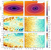 |
Fig. 1. Surface brightness contours (upper panels) of NGC 4550 (left) and NGC 2768 (right). The middle and lower panels show the v/σ maps constructed with the Gauss Hermite and non-parametric kinematics, respectively. |
In addition to moment maps, we can also visualise the stellar kinematics as channel maps for the non-parametric dataset, as is shown in Figs. 2 and 3. Channel maps are commonly used in radio observations and show the same image in different velocity intervals (for example, see Fig. 3 in Nakashima et al. 2009). While it is possible to construct such channel maps for parametric kinematics as well, they are not as straightforward to interpret, as the parametric LOSVDs are not defined as a probability distribution and hence can contain negative values at given velocities. For the non-parametric LOSVDs, the channel maps can be constructed by simply plotting the densities given by the histogram in the individual velocity bins. These bins – as defined in Bayes-LOSVD – give the velocity intervals of the channel maps4.
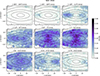 |
Fig. 2. Channel maps constructed from the non-parametric stellar kinematics of NGC 4550 over all spatial bins in different velocity intervals. The percentage of the contribution of each spatial bin to the specified velocity bin is colour-coded (see colour bar at right). |
For NGC 4550, the top right panel of Fig. 2 shows the prominence of the counter-rotating stellar disks at high negative velocity, while the bottom second panel is dominated by the regularly rotating disk at high positive velocity. These regions of high densities at high and low negative velocities in turn do not significantly contribute at v = 0 km/s in comparison to the rest of the galaxy (middle second and third panels) and are located in the same bins, where the v/σ map constructed from the Gauss Hermite kinematics indicates the counter-rotating disks in the middle left panel of Fig. 1.
The channel maps for NGC 2768 are shown in Fig. 3. The highest density for negative and positive velocities moves from the right (upper panels) to the left (lower panels) side of the galaxy, consistent to the information contained in the middle and lower right panels of Fig. 1. All results for this galaxy indicate regular rotation.
To investigate the difference between the two v/σ maps of NGC 4550, we also look at the resulting LOSVD shapes directly. For a broad overview of the whole galaxy, the upper panels of Fig. 4 show bimodality maps for NGC 4550, where the colours indicate the number of peaks detected in the Gauss Hermite (upper left panel) and non-parametric (upper right panel) LOSVDs, respectively. The number of peaks in the LOSVDs are determined with the find_peaks function in scipy. The grey bins correspond to unimodal LOSVDs and the black bins to bimodal shapes. The black bins in this map therefore highlight the regions where the counter-rotating stellar disks are resolved in the non-parametric kinematics. These bins correspond to those regions (at small |y| and large positive and negative x) in the middle left panel of Fig. 1, where the counter-rotating disks are indicated in the v/σ map of the Gauss Hermite kinematic data. In contrast, the peak map constructed with the Gauss Hermite kinematics (upper left panel) uniformly shows unimodal LOSVD in each spatial bin, indicating that this counter-rotating substructure is not well resolved directly in the parametric LOSVDs.
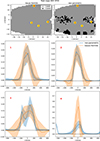 |
Fig. 4. Bimodality maps (upper panels) of NGC 4550 and comparison of different Gauss Hermite and non-parametric LOSVD shapes for four example spatial bins. |
To illustrate this further, the bottom four panels in Fig. 4 show a direct comparison between the LOSVDs resulting from the two different extraction techniques at the same spatial bin. The shaded regions correspond to the 68% credibility intervals for the respective LOSVDs. For the non-parametric kinematic data, this uncertainty interval results directly from the posterior sampling. For the Gauss Hermite kinematic data, we Monte Carlo sampled 500 sets of kinematic parameters from their uncertainty ranges derived from the spectral fit, and evaluated LOSVDs using these parameters. We then took the mean of these 500 LOSVDs to describe the best-fit. For comparison with the non-parametric uncertainty range, we also took the 68% credibility interval from the range of samples.
The middle left panel of Fig. 4 shows similar LOSVD shapes for the two kinematic sets. Both indicate a classical Gaussian shape of the LOSVD in this spatial bin. We do note, however, that the Gauss Hermite LOSVD is slightly broader. The sudden drop in the contribution to the LOSVD (that is the steepness of the slope) found in the non-parametric LOSVD is not represented in the parametric result. Additionally, the mean estimate of the Gauss Hermite LOSVD is positive but the uncertainties indicate potential negative contributions. For the non-parametric LOSVDs the uncertainty intervals are constrained to be non-negative. The middle right panel of Fig. 4 again shows similar results of the Gauss Hermite and non-parametric LOSVDs in the centre regions of the galaxy. However, this panel shows the issue of negative values in the Gauss Hermite distribution. They imply a negative number of stars at a given velocity, which is unphysical. This problem becomes more relevant at higher order in the Gauss Hermite expansion. See Appendix A for more detailed discussion.
The bottom left panel shows the mischaracterisation of the Gauss Hermite LOSVD as unimodal in a region where counter-rotation is suggested in both the non-parametric kinematics and the v/σ map of the Gauss Hermite kinematics. This results in a significant overestimation of σ in the parametric LOSVD. While the Gauss Hermite LOSVD is noticeably skewed towards positive velocities, it does not directly resolve the two counter-rotating stellar components in that region of the galaxy. This occurs in all regions where the non-parametric kinematics resolve bimodal LOSVDs. Overall, the Gauss Hermite description of the kinematics therefore produces significantly broader shapes in the velocity distribution.
At this point, we again point out that there are options within pPXF to fit multiple kinematic/stellar population components, with which it is possible to explicitly recover counter-rotating disks. This has been done for NGC 4550 in Johnston et al. (2013) and, for example, for multi-component fits to stellar continua for thin/thick disk systems in Shetty et al. (2020). While this is useful to relax unimodal assumptions inherent to single component parametric LOSVD reconstruction, this approach is usually only used if the single-component fits do not work at all or if there are some prior indications about the kinematic complexity of the observed objects. This is because the two-component fit is less straightforward and more complicated in terms of uncertainty estimation than the single-component fit. Therefore, we have chosen to take the default approach to fitting with pPXF, by fitting only one component. With Bayes-LOSVD, more complex LOSVD shapes are automatically recovered in the fitting process without adding options for multiple components. This may improve the success rate of recovering kinematically complex systems, as the same procedure can be applied to all galaxies without manually adjusting the number of components to fit.
One issue that we find for the non-parametric LOSVDs is indicated in the bottom right panel of Fig. 4. In some cases of the outermost spatial bins, where the data are noisier (hence the data have a lower S/N), the non-parametric kinematics show sudden spikes at the highest or lowest velocity bin. It is currently unclear why exactly these spikes occur. The bottom right panel of Fig. 4 shows one such spike at v = −600 km s−1, which leads to a broader LOSVD and hence higher velocity dispersions in the affected regions. In Appendix B, we show the spectrum fits with Bayes-LOSVD in the four regions of Fig. 4. The lowest spectrum fit in the left panel of Fig. B.2 corresponds to region 4 and clearly shows that the fit in this spatial bin is not very good. We did additional, regularised non-parametric fits (Appendix D) to investigate if regularisation limits the issue of the spikes and find that while there are still some outer bins where these spikes at large |v| occur, the total number of such cases decreases. To account for the regions where the spikes appear in our main analysis, we manually inflated the uncertainty by a factor of 10 in cases where the two outer velocity bins contribute more than 3% to the LOSVD to ensure that they do not overly bias the dynamical inference. We point out that this does not properly correct for the spikes in the wings, as the normalisation of the LOSVD will change if the power in the wings is moved into the main LOSVD. For a better handle on these spikes, it will be necessary to find a good balance for flexibility in the LOSVD shape and regularisation to enforce some level of smoothness.
The bimodality map for NGC 2768 is uniformly unimodal from the Gauss Hermite kinematics. Interestingly, the non-parametric kinematics do indicate several spatial bins with bimodal LOSVDs (see Fig. B.6, for more discussion see Appendix B). It is not immediately evident if these signatures are tracking specific substructures or if they are random noise being detected by the find_peaks function. This, together with the unphysical spikes in the tail at some outer spatial bins, again highlights the current limitations of the non-parametric LOSVD recovery in terms of including realistic regularisation. Overall however, the LOSVDs of NGC 2768 are mainly Gaussian-shaped in both cases, making the difference between the Gauss Hermite and the non-parametric kinematics negligible in comparison to NGC 4550, as already indicated in the v/σ maps in the right column of Fig. 1.
4. Dynamical inference: Method
There are different methods of dynamical modelling of stellar systems or galaxies based on observed stellar kinematics. All of them constrain the enclosed mass within the observed radius, as the stellar kinematics trace the underlying gravitational potential. The asymmetric drift correction (Binney & Tremaine 1987; Weijmans et al. 2008) uses the Jeans equation and the thin disk assumption to determine the enclosed mass. The Axisymmetric Jeans Anisotropic Multi-Gaussian expansion (JAM) model (Cappellari 2008) does not use the thin disk assumption and can provide the enclosed mass and the velocity anisotropy. Made-to-measure N-body simulations can be used to simulate particles representing (sets of) stars (Syer & Tremaine 1996). To model the internal structure of galaxies, however, there are a limited number of options. Orbit-superposition modelling based on the numerical models of Schwarzschild (1979, 1982) are typically used for recovering the full orbit structure and the intrinsic shape of an observed galaxy, along with its enclosed mass.
As the main aim of this work is to investigate differences in the dynamical inference of both the mass and the orbital structure caused by the type of stellar kinematics, we applied a recent implementation of triaxial orbit-superposition modelling DYNAMITE (DYnamics, Age and Metallicity Indicators Tracing Evolution; Jethwa et al. 2020; Thater et al. 2023)5 to both reconstructed LOSVDs.
DYNAMITE is an implementation of the orbit-superposition technique (Schwarzschild 1979, 1982) for modelling triaxial systems. The full method is described in van den Bosch et al. (2008), van de Ven et al. (2008). This section provides a brief overview of the method and our set-up. As this is the first description of how the results of Bayes-LOSVD are implemented, we also give a more detailed description of the application to the LOSVDs constructed from both Gauss Hermite and non-parametric methods, respectively.
4.1. Methods: DYNAMITE
The main assumption in dynamical modelling is that the gravitational potential does not change significantly during the time that the orbits are integrated. The main steps in the orbit calculation with DYNAMITE are the following:
-
Define a gravitational potential by setting up the hyper-parameter space (including dark and baryonic components);
-
Integrate a variety of orbits in the potential;
-
Find the optimum orbit weights so that the superimposed orbits reproduce the observables;
-
Change the potential and repeat.
Generally, the hyper-parameter space consists of the stellar mass-to-light ratio Υ, the super-massive black hole mass, the scale length of the analytic black hole potential, the dark matter fraction, and the intrinsic shape parameters p, q, u6. For our analysis, we searched the parameter space of Υ (in the parameter range 0.5−6 M⊙/L⊙ for NGC 4550 and 2−6 M⊙/L⊙ for NGC 2768) and two of the shape parameters, specifically p and q in the ranges 0.5−0.99 (0.6−0.8) and 0.1−0.99 (0.2−0.4) for NGC 4550 (NGC 2768). We note that the parameter ranges are narrower for NGC 2768, as we used constraints from Thater et al. (2023) for this galaxy.
As both galaxies visually appear axisymmetric, we fixed u to 0.99 for both galaxies. Additionally, we kept the black hole mass and the dark matter fraction M*/M200 parametrised by the dark matter halo mass M200 7 fixed in both galaxies to limit the number of free parameters.
Together with the surface brightness profile of the galaxy, which provides a representation of the stellar density distribution, we used these parameters to calculate a model of the gravitational potential. Within this model potential, we integrated the orbit library. The size of the orbit library is given by the numbers of the starting locations conserving the three integrals of motion, that is energy E, I2, and I3. We set nE = 21, nI2 = 10, and nI3 = 7. In addition, we mirror the orbits, which increases the size of the orbit library without additional integration, and include an additional set of box orbits. This triples the size of the orbit library, so that norbs = 3 ⋅ nE ⋅ nI2 ⋅ nI3 = 3 ⋅ 21 ⋅ 10 ⋅ 7 = 4410. In order to smoothen the orbit distribution, the orbit positions are dithered by a number of 5, increasing the sampled three-integral space by 53 (as dithering creates orbit-bundles)8. We integrate the orbits over 200 circular orbital periods.
We then solve for the weighted linear combination of orbits best fitting to the mass distribution and the kinematic observations. This is done by minimising the difference between the projected quantities of the data (surface brightness and kinematics) and the model. This process is iterated several times for different values of the hyper-parameters to select the best fitting gravitational potential. This is done via grid-search, by setting minimum and maximum limits for each parameter. The choice of the fit metric to select the best-fit model for the two types of kinematic input is different. This is discussed in more detail in Sects. 4.2 and 4.3. We ran the models on the Vienna Scientific Cluster9. Depending on the number of spatial bins, calculating one Schwarzschild model (that is, one set of parameters describing one gravitational potential) takes around 2 hours using 128 CPUs.
Table 1 shows an overview of the individual simulation runs we performed. The main analysis in Sect. 5 concerns NGC 4550 and NGC 2768 both binned to S/N = 60 for both kinematic sets. In addition, we aimed to test different effects of the kinematic input on the dynamical inference. For the counter-rotating galaxy NGC 4550, we tested how much the spatial binning of the observed spectrum affects the dynamical inference based on the two kinematic sets. In this run, we used the spectrum binned to S/N = 150, resulting in significantly fewer spatial bins than in the main analysis, where we used S/N = 60. We also ran DYNAMITE on regularised non-parametric kinematics to account for differences in the dynamical inference caused by regularisation, see Appendix D for more details. For all simulation runs, we used the same set-up as described above.
DYNAMITE runs performed with the respective kinematic input for NGC 4550 and NGC 2768.
4.2. Using Gauss Hermite kinematics in DYNAMITE
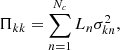
We set the type of weight solver for the Gauss Hermite input as LegacyWeightSolver in DYNAMITE, which uses a Fortran implementation of the Lawson & Hanson (1995) Non-Negative Least Squares algorithm. For model selection, we used the χ2 arising purely from the kinematic constraints (i.e. excluding the supplementary surface- and mass-density constraints). For the parametric kinematics, this yields two options for χ2 during the weight solving procedure, namely χkin2 and χkinmap2. These two are similar in theory, as both indicate the goodness-of-fit, but are calculated differently. The best fitting set of hyper-parameters is chosen based on the approach in Zhu et al. (2018), using the χ2 value of each model, derived in the following way:
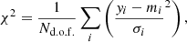 (1)
(1)
where yi are the observed kinematics, mi the model kinematics, and σi give the observational error, normalised by Nd.o.f., the total number of degrees of freedom in the model. In the Gauss Hermite case, this is the number of spatial bins times the number of Gauss Hermite moments. For the definition of χkinmap2, the parameters yi and mi are given by (v, σ, h3, h4) in each spatial bin. In contrast, the definition of χkin2 uses the parameters (h1, h2, h3, h4).
χkin2 is used to compute the orbit weights, fixing v and σ to the observed values, and fitting h1 and h2 along with the (specified) higher-order moments to describe the LOSVDs produced by the orbits in the apertures. The minimisation approach follows the description using Eq. (1). χkinmap2 is derived from the already weighted combination of orbits and fits v and σ along with the Hermite coefficients of order 3 and up, fixing h1 and h2 to zero, as is done in pPXF during the calculation of the Gauss Hermite moments. For Eq. (1), yi and mi would therefore be made up of v, σ, and the Gauss Hermite moments of orders h3 and up.
The choice of using χkinmap2 or χkin2 results in a difference in the model selection. We point out the importance of clearly stating which fit metric is chosen. For our analysis, we consistently use the χkinmap2-selected results, as these showed the least difference between the Gauss Hermite and the non-parametric results. For a discussion of the differences in the model results caused by the two fit metrics, see Appendix C.
4.3. Using non-parametric kinematics in DYNAMITE
This section describes the implementation of orbit-based modelling with non-parametric kinematics in DYNAMITE. Non-parametric kinematic measurements output by the Bayes-LOSVD software (Falcón-Barroso & Martig 2021) can be provided as inputs to DYNAMITE. These measurements consist of the posterior median (yij) and 68% credibility interval (σij) of inferred LOSVDs for some user-defined velocity bins (indexed i = 1, …, Nv) and spatial bins (indexed j = 1, …, Ns). Within DYNAMITE, orbit-bundles (indexed k = 1, …, Nb) are binned in the same way as the measurements. We represent the orbit-bundles as a 3D-array gijk which encodes the contribution of orbit-bundle k in spatial bin j and velocity bin i. These are normalised such that each orbit-bundle sums to one when integrated over spatial and velocity co-ordinates.
We next construct a set of linear equations to solve for the unknown orbit-weights wk. The non-parametric kinematics provide a total of Nv × Ns constraints of the form
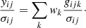 (2)
(2)
As is done for Gauss Hermite kinematics (van den Bosch et al. 2008), these kinematic constraints are supplemented by two sets of additional constraints to enforce self-consistency. The first set enforces that the solution matches the observed surface density within Ns spatial bins. The second set enforces that the solution matches the de-projected mass-density on a 3D-grid which has, by default, 360 grid cells. Altogether, this gives Nc = (Nv + 1)Ns + 360 constraints, which are arranged into a matrix with Nc rows and Nb columns. We solve this matrix equation using the scipy non-negative least squares (NNLS) function, which implements the fast NNLS algorithm (Bro & De Jong 1997) which is based on the Lawson & Hanson (1995) algorithm.
The relevant χ2 calculation is the same as Eq. (1), but now Nd.o.f. is equal to the number of velocity bins times the number of spatial bins, yi corresponds to the velocity bins from the observations, and mi to those from the model LOSVD. As before, σi gives the respective observational error. In contrast to the Gauss Hermite case, for non-parametric kinematics we avoid the issue of having to choose between two different options of χ2 for model selection. We also point out that the χ2 values resulting from the two sets of kinematic input are not quantitatively comparable with each other due to the different values of Nd.o.f..
5. Dynamical inference: Results
In this section, we discuss the differences in the dynamical inference caused by the type of LOSVD description. In the following analysis, the uncertainties are given by the range in the hyper-parameter space covered by the 50 best-fit models of the respective runs. These are also used to evaluate and compare the goodness-of-fit of the non-parametric and the Gauss Hermite dynamical models, as the uncertainties depend on how well the dynamical models fit the data (that is, a large scatter in the hyper-parameters results in a larger uncertainty and vice versa.) We are not comparing the χ2 values directly, as they are calculated differently for the two inputs, as explained in the previous section. For visualisation purposes, we include the χ2 map of the best-fit non-parametric models and the residual maps of the best-fit Gauss Hermite models for NGC 4550 and NGC 2768 in Figs. B.4 and B.5, respectively. Overall, both methods result in a good fit to the data.
5.1. Best-fit hyper-parameters
As Table 2 shows, there are small differences in the best-fit values for the intrinsic axis ratios p and q of NGC 4550 between the models based on Gauss Hermite and non-parametric kinematics, respectively. Cappellari (2002) argue that the shape is mainly determined by the MGE. During the modelling, we find that q is constrained to small values by the MGE, that is, by the inclination angle of the galaxy. The dark matter fraction in both model results is constrained to the same value. The most significant difference appears in the stellar mass-to-light ratio Υ, where the non-parametric case yields Υ = 2.88 M⊙/L⊙, while the parametric result gives Υ = 4.25 M⊙/L⊙, as shown in Table 2. In Sect. 5.2, we compute the enclosed mass profile from Υ.
Comparison of global values for the best-fit parameters, velocity anisotropy parameters, and relative contributions of different orbit types of NGC 4550.
For NGC 2768, Υ = 5.80 M⊙/L⊙ for the Gauss Hermite and Υ = 5.60 M⊙/L⊙ for the non-parametric kinematics (see Table 3), showing a smaller difference than for NGC 4550. This fits with our initial expectation, as this galaxy is a regular rotator and the difference in the LOSVDs is smaller, as described in Sect. 3.3. The most notable difference for the hyper-parameter space of this galaxy is in the shape parameter p, with a relative difference of around 10%. We note that the uncertainties for this case are quite small, which is likely caused by the smaller parameter range in p to be searched for this galaxy in comparison to that of NGC 4550 (Sect. 4) while using the same step size. While the range is the same for Gauss Hermite and the non-parametric case, we find only little variation in p.
To account for any potential missing models in the respective DYNAMITE runs, we also tested the goodness-of-fit for the Gauss Hermite kinematics but with the best-fit parameters from the non-parametric result. The kinematic maps show a significantly worse agreement between the observational data and the model in this case. The large σ values in regions of overlapping stellar disks (see e.g. bottom left panel of Fig. 4) result in a significantly different choice of the best set of parameters and, hence, a different gravitational potential compared to the models inferred from the non-parametric kinematics.
5.2. Enclosed mass profile
Figure 5 shows the enclosed total mass profiles of the models. The left panels shows NGC 4550, where the enclosed mass estimate of the non-parametric kinematics is significantly lower than for the Gauss Hermite case while the uncertainty regions show some overlap. We compare the results of our dynamical model to those of the Schwarzschild modelling of NGC 4550 by Cappellari et al. (2006, 2007) and to the M2M models of Long & Mao (2012). We note that the difference between their slope and the slope of our Gauss Hermite curve is likely caused by the different MGEs. They created the MGE from V-band photometry, while our results are based on the r-band photometry of Scott et al. (2013). To calculate the respective mass profiles, we used our best-fit parameters for deprojection of their MGE parameters (taken from the Appendix of Cappellari et al. 2006)10. Both comparison cases used the same Gauss Hermite kinematics as input for their subsequent modelling. The enclosed mass profiles of the two comparison cases lie slightly above the upper limit of the uncertainty in mass from the non-parametric models and within the uncertainty region of our Gauss Hermite case.
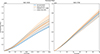 |
Fig. 5. Enclosed mass profiles for NGC 4550 (left) and NGC 2768 (right) resulting from Gauss Hermite parametrisation (orange) and the non-parametric description of the kinematics (blue). For NGC 4550, the comparison includes the results of Cappellari et al. (2006) (solid line) and Long & Mao (2012) (dashed line). |
We argue that the reason for the significant difference in the total mass is due to the overestimation of σ in the Gauss Hermite parametrisation of the LOSVD, which – due to the presence of two counter-rotating disks – is non-Gaussian. As demonstrated in the bottom left panel of Fig. 4, this leads to a broad LOSVD, that is, a high σ. Due to the relation between the velocity dispersion and the stellar mass, this results in a similarly larger value of the total mass.
This is further supported by the fact that we do not find a significant difference in the mass profiles for NGC 2768 (right panel of Fig 5). The extracted stellar kinematics are more similar and therefore the dynamically inferred masses are the same. It is only in the outer regions of the galaxy (at around 15 arcsec) that the masses start to diverge slightly. This difference is small but again the Gauss Hermite kinematics suggest a slightly higher total mass. In comparison with the uncertainties, however, this difference is negligible.
5.3. Shape profile
Figure 6 shows the shape profiles resulting from the dynamical models with the Gauss Hermite and the non-parametric kinematics. Alongside p and q, Fig. 6 also indicates the triaxiality  . The left panel shows the results for NGC 4550. As we have fixed u = 0.99, both kinematics sets result in a nearly axisymmetric system, with the non-parametric model suggesting a slightly less triaxial shape. This is caused by a higher p value. However, for both p and T this difference lies within the error bars of both the non-parametric and the Gauss Hermite results. We note that fixing u = 0.99 means that the intermediate axis of the galaxy is projected along the line of sight, which may impart a bias on the model selection. As we make this assumption for all our models, any differences caused by the different kinematic methods are not affected by this. The fixed u parameter however does put a caveat on any derived physical parameters of our models, as they may vary slightly under the assumption of a different u value.
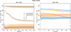 |
Fig. 6. Shape profiles of NGC 4550 (left) and NGC 2768 (right), where p (dotted line) and q (dashed line) are two axis ratios and T (solid line) gives the triaxiality of the galaxy. For both galaxies, the difference between the two methods is most apparent in p, which translates into T. |
Interestingly, we find a more significant difference for NGC 2768 (right panel of Fig. 6). Again, the models resulting from the non-parametric kinematics prefer a slightly less triaxial model, due to higher values for p. However, the difference in both parameters is notably larger than in the case of NGC 4550 and the values of the two models lie outside their respective uncertainty ranges. This is curious as the shape profile is mainly determined by the MGE (Cappellari 2002), and the same are used for our dynamical modelling of both the Gauss Hermite and the non-parametric kinematics. It is therefore likely that it is the difference in the stellar orbits that result in a different triaxial shape of the galaxy. We discuss this in more detail in Sects. 5.5 and 6.2.
5.4. Velocity anisotropy
For the velocity anisotropy parameters, we use βz and βr, as described in Binney & Tremaine (1987) and Cappellari et al. (2007) in the following way. With the dispersion tensor σkn described as
we can derive
 (3)
(3)
where Ln is the light contained in each of the Nc spherical bins of the model. Depending on the coordinate system, we use either the spherical (r, Φ, Θ) or cylindrical coordinates (R, Φ, z) for k, n. We then write
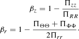 (4)
(4)
The resulting velocity anisotropy profiles of both galaxies are shown in Fig. 7.
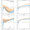 |
Fig. 7. Spherical (upper row) and cylindrical (bottom row) velocity anisotropy profiles of NGC 4550 (left column) and NGC 2768 (right column) resulting from the dynamical models using the Gauss Hermite kinematics (orange) and the non-parametric kinematics (blue), respectively. |
In the upper left panel of Fig. 7, we see that, for NGC 4550, βr from both kinematic types follow the same trend, with the non-parametric results showing more negative values, especially in the innermost region of the galaxy. This strong gradient at small r is likely caused by the two stellar disks. Similarly, the radial profiles of βz suggest less tangential velocity anisotropy for the Gauss Hermite results. In this case, the trend only becomes similar at around 12 arcsec, while in the inner regions the non-parametric results show a significantly negative tangential velocity anisotropy. From this, we expect more dynamically cold orbits in the non-parametric models, as they would be rotation-dominated and less radial.
The right panels of Fig. 7 show the anisotropy parameters of NGC 2768. While the difference in the innermost regions is less pronounced than in the case of NGC 4550, the non-parametric models again show smaller βr and βz values throughout the galaxy. As for NGC 4550, the Gauss Hermite models have higher-velocity anisotropies, suggesting more radial, less rotation-dominated orbits. This is consistent with the results of the right panel of Fig. 6, which also indicate more dispersion-dominated stars in the Gauss Hermite case due to the more triaxial shape of the galaxy.
For NGC 4550, we also compare our global anisotropy parameters (averaged over the radius, see Table 2) to those of Cappellari et al. (2006), Long & Mao (2012): The results are largely consistent between the models, the most significant difference occurs for the spherical anisotropy of our Gauss Hermite models, resulting in a global βr = −0.08, while βr = −0.40 for our non-parametric case and βr = −0.37 and βr = −0.26 for Cappellari et al. (2006) and Long & Mao (2012), respectively. Comparing the global values for NGC 2768 Table 3, we find that the cylindrical velocity anisotropy βz is consistent between the two models, while the spherical velocity anisotropy βr is smaller for the non-parametric kinematics by 1/4. Overall, the Gauss Hermite models show a more radial anisotropy globally.
5.5. Stellar orbits
We separate the orbit libraries resulting from the best-fit models to the two kinematic sets for both galaxies into the different orbit types, based on their angular momentum components (Lx, Ly, Lz). We separate the orbits into 4 types: Boxes, where all angular momentum components are close to 0, long (x) axis tubes, where |Lx| is the largest component, intermediate (y) axis tubes, where |Ly| is the largest component, and short (z) axis tubes, where |Lz| is the largest component. Box orbits are mainly dispersion-dominated, while tube orbits are mainly rotation-dominated. We point out that the intermediate axis tubes are unstable and therefore not present in real systems, while long axis tubes generally make up a relatively low percentage of orbits. We find that their contribution to the orbit libraries are small. The global values of the relative orbit fractions calculated from the best-fit models of for both galaxies are given in Tables 2 and 3, respectively. Figure 8 shows the radial profile of the percentage of box and short axis tube orbits for NGC 4550 (left panel) and NGC 2768 (right panel).
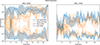 |
Fig. 8. Relative orbit fractions for the short axis tubes (solid lines) and the box orbits (dashed lines) from the Bayes-LOSVD (blue) and Gauss Hermite (orange) models, respectively, for NGC 4550 (left) and NGC 2768 (right). |
In NGC 4550, the short axis tubes dominate in every region of the galaxy in the non-parametric models. For the Gauss Hermite models, however, the box orbits dominate in the inner regions of the galaxy, out until around 5 arcsec. In the outer regions, the orbit fractions are more similar. This is consistent with the anisotropy profiles in the left panels of Fig. 7, where the inner regions also show the biggest differences. This is likely caused by the two stellar disks prominent in the inner regions of this galaxy, which are better resolved in the models resulting from the non-parametric kinematics. Similarly, both the anisotropy profile and the orbit fractions indicate more dispersion-dominated orbits in the Gauss Hermite models. In these cases, the model provides a higher fraction of box orbits to account for the broad LOSVDs (compare bottom left panel of Fig. 4). This higher fraction of box orbits also leads to the higher total mass we find in Fig. 5. As Table 2 shows, the number of box orbits in the Gauss Hermite models is almost twice as high as in the non-parametric models.
The right panel of Fig. 8 shows NGC 2768, which overall has a lower fraction of short axis tube orbits than NGC 4550, but a comparable amount of box orbits. Similarly to NGC 4550, it is again the innermost regions of NGC 2768 with the most significant difference in the short axis tube fractions between the Gauss Hermite and the non-parametric models, although the discrepancy is less extreme for this galaxy. This is also consistent with the anisotropy profiles in the right panels of Fig. 7. However, as indicated in Table 3, while the difference in the global short axis tube fractions is comparable to that of NGC 4550, the difference in the box orbits fraction is smaller, only 5%. From this we conclude that the difference in the velocity dispersions between the two models is significantly smaller than for NGC 4550. This is consistent with the difference we find in the mass profiles between the two galaxies (Fig. 5).
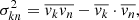
In order to analyse the difference in rotation and dispersion in more detail, we also show the one-dimensional short axis tube orbit distributions of the two galaxies in Figure 9. The x-axis gives the circularity parameter 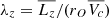 with averaged Lz, rO2 = x2 + y2 + z2, and
  . For Fig. 9, we have integrated λz along the time-averaged radius r. Based on this distribution, we separate the galaxy into dynamically cold (rotation-dominated), warm, hot (dispersion-dominated), and counter-rotating components by 0.75 < λz ≤ 1, 0.25 < λz ≤ 0.75, −0.25 ≤ λz ≤ 0.25, and −1 ≤ λz < −0.25, respectively. We note that the Gauss Hermite and non-parametric orbit distributions are normalised the same way for NGC 4550 and NGC 2768, respectively.
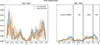 |
Fig. 9. One-dimensional circularity distribution of the short axis tube orbits of NGC 4550 (left) and NGC 2768 (right) resulting from the non-parametric (blue) and the parametric (orange) kinematics. |
For NGC 4550, the most significant difference between the two models is in the counter-rotating component. For the non-parametric case, most of these orbits cluster near λz = −1, indicating a dynamically cold counter-rotating disks, see the left panel of Fig. 9. For the Gauss Hermite result, we also find a clear indication for a counter-rotating component. The models, however, suggest a dynamically warmer secondary disk. At positive λz, the peak is more similar to the non-parametric result, but it is also located at a slightly smaller |λz|, implying more dispersion-dominated orbits. This, together with the generally higher fraction of box orbits, is likely accommodating the Gauss Hermite model’s preference for a higher Υ, which is in turn causing the difference in the total mass in the left panel of Fig. 5, assuming that both models fit equally well to their respective data. Figure B.4 shows how the best-fit model fits the data and we clearly see that the regions where the counter-rotating disks occur are fit very well both for the non-parametric (for this compare also Fig. 10) and the Gauss Hermite model.
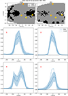 |
Fig. 10. As in Fig. 4, but the top left panel shows the bimodality map of the best-fit model of NGC 4550. The middle and bottom panels show the LOSVDs of the data (solid lines) and the model (dashed lines) of the same spatial bins as in Fig. 4. |
The right panel of Fig. 9 shows the short axis tube orbit distribution for NGC 2768. We see that the number of short axis tubes in this galaxy is significantly smaller than for NGC 4550. The small counter-rotating fraction is similar for both models, the non-parametric results only indicate a slightly stronger counter-rotating component. In this galaxy, the main difference is found at positive λz, where the Gauss Hermite results again indicate a dynamically warmer disk than what we find for the non-parametric results. As for NGC 4550, this is consistent with the shape and anisotropy profiles (right panels of Figs. 6 and 7), respectively. These differences in the short axis tube orbit distribution are likely negligible due to the generally small differences in the overall orbit fractions between the Gauss Hermite and the non-parametric results, leading to the similar values for Υ and hence more similar total mass estimates (right panel of Fig. 5).
5.6. Updated properties of NGC 4550 and NGC 2768
Overall, we find that the non-parametric kinematics suggest dynamically colder, hence thinner, disks for both galaxies. This is most influential for NGC 4550, where this leads to a significantly lower total mass than previous results using the Gauss Hermite kinematics. The galaxy’s total mass derived from the non-parametric models is around (7.5 ± 0.3)⋅109 M⊙ within 20 arcsec. We use cuts at λz = ±0.75 to select disks orbit. Then, the two dynamically cold counter-rotating disks can be easily separated, and their individual masses can be calculated. In total, the two dynamically cold stellar disks account for roughly 40% of the total orbit weights in the non-parametric models, i.e. slightly less than half of the galaxy’s total mass resides in the two thin disk components. Assuming a constant Υ for all dynamical components in the galaxy, we therefore calculate an estimate for the total mass of the prograde disk to be around 1.7 ⋅ 109 M⊙, and for the mass of the retrograde disk 1.4 ⋅ 109 M⊙ 11. This is consistent with Coccato et al. (2013), who find that the secondary component is slightly less massive than the main component of the galaxy. However, we note that Johnston et al. (2013) have found evidence for an age difference of around 8 Gyr between the two stellar disks. Therefore, it is likely that different stellar mass-to-light ratios appropriate for different stellar populations would need to be used for more accurate estimates of the mass of the two disks.
6. Discussion
In this section, we discuss the cause of the differences in the dynamical inference resulting from the parametric and the non-parametric descriptions of the stellar kinematics, as well as their limitations as input for dynamical modelling.
6.1. Bimodality in model LOSVDs
To investigate how well the dynamical models reconstruct the kinematic substructures from the input data, we also constructed the bimodality maps (as shown in the upper panels of Fig. 4) for NGC 4550 and NGC 2768 from the best-fit models. We perturbed the model LOSVDs with the uncertainty from the kinematic inference and locate those spatial regions, where the model suggests substructures by locating the bins indicating more than one peak in the LOSVD (again determined using the find_peaks function).
For NGC 4550, we find that the non-parametric model clearly resolves bimodal structures in the LOSVD in the same regions indicated by the data, compare the upper panels of Fig. 10. As can be seen in the bottom left panel, the model LOSVDs also show bimodal shapes which are consistent within the errors. On the other hand, the peak maps are flat at one peak for both the Gauss Hermite model and data. We do not show either here, as the bimodality maps are generally more meaningful for the non-parametric case by construction due to the higher flexibility in LOSVD shapes. While the orbit distribution (left panel of Fig. 9) suggests counter-rotating stellar disks, this structure is not recovered in the LOSVDs of the model, similar to the input data. Rather, these are again suggesting broad unimodal LOSVD shapes, resulting in the higher total mass.
For NGC 2768, the Gauss Hermite model and data again show flat bimodality maps, indicating no notable kinematic substructures. Interestingly, the non-parametric model LOSVDs do indicate some spatial regions with slightly bimodal LOSVDs. However, similar to the map constructed from the non-parametric kinematic data (see Sect. 3.3), these regions do not seem to form coherent structures. Rather, they are seemingly randomly distributed within the galaxy. It may be that the non-parametric recovery is either picking up very faint substructures or random noise, which is then reproduced in the model LOSVDs. Either way, the signal is not strong enough to cause a significant difference in the mass or the orbit distribution of that galaxy.
6.2. Effect of non-parametric kinematics in dynamical inference
Connecting our findings on the dynamical biases caused by parametric stellar kinematics, we see that the current description using Gauss Hermite expansion is not flexible enough to adequately recover significant deviations from Gaussian shapes of the LOSVD. Examples of such cases are counter-rotating galaxies or galaxies with other dynamical substructures, such as rings or bars, or stellar streams. Even if the moment maps of the Gauss Hermite expansion give an indication of these substructures when they are significant enough (for example the counter-rotation of NGC 4550 being captured in the v/σ map in the middle left panel of Fig. 1), it is not possible to properly resolve these substructures directly in the LOSVDs (bottom left panel of Fig. 4). Instead, they appear broader in regions of the galaxy where the substructures exist, resulting in an overestimation of the velocity dispersion σ.
We find that this has a significant effect on the dynamical inference, namely on the choice of gravitational potential, the recovered orbit solution, and the estimated mass. The dynamical models calculated from the Gauss Hermite kinematics prefer an orbit library populated with relatively more box than tube orbits. This implies larger weights for the dispersion-dominated orbits (Fig. 8). As the circularity of these orbit types is on average lower than that of the rotation-dominated orbits, the parametric kinematics model suggests dynamically warmer, thicker disks than the non-parametric kinematics model, as shown in Fig. 9. Figures B.4 and B.5 show that both best-fit models fit their respective datasets (Gauss Hermite and non-parametric kinematics) similarly well.
Hence, the preference for a more dispersion-dominated galaxy is likely what is causing the difference in the inferred mass of NGC 4550 (left panel of Fig. 5). The smaller difference in the mass estimate of NGC 2768 can be explained by the comparatively smaller fraction of rotation-dominated orbits in both models (see y-axis in the right panels of Figs. 8 and 9). While this overall difference in the orbit distributions leads to inconsistent values in the anisotropy parameters and the shape, it is not large enough to affect the mass estimate. It is likely that the shape profile shows a larger discrepancy between the two models for NGC 2768 because of the smaller variation range we adopted for this galaxy and the higher fraction of long axis tubes (compare Table 3). This is supported by the fact that the shape profiles for NGC 4550 are more consistent - the number of long axis tube orbits is negligibly small. Concerning the velocity anisotropy, the higher weight on the dispersion-dominated orbits in the Gauss Hermite models results in more radial anisotropy for both galaxies. This is more so the case for NGC 4550, especially in the inner regions, where we correspondingly find a high fraction of box orbits, but also noticeable for NGC 2768. In the case of more regular stellar kinematics, we therefore still find some differences in the recovered dynamical structure, even if the mass estimate is less affected.
Since the non-parametric kinematic recoveries are not limited to nearly Gaussian shapes and therefore do not bias σ in the same way as in the Gauss Hermite expansion, we argue that they are more reliable in terms of the results from subsequent dynamical inference. A σ value that is biased high cannot only inflate the mass estimate but also results in other biased observational quantities, such as v/σ, which is used to separate slow and fast rotators (Cappellari et al. 2007; Emsellem et al. 2007).
We conclude that the use of non-parametric kinematic recoveries for galaxies with complex kinematics (e.g. counter-rotation, but also bars, ring structures) is advantageous to resolve kinematic substructures better. These also yield results of the dynamical inference which are more consistent with these substructures. We suggest moving towards the use of non-parametric kinematic descriptions in the dynamical studies of all kinds of galaxies, as we also find notable differences in the orbit fractions and distribution of supposedly regular rotator NGC 2768.
6.3. Effect of signal-to-noise
To investigate whether the spatial binning of the spectra has any effect on the dynamical inference, we binned NGC 4550 to a higher S/N of 150 in the non-parametric kinematic recovery. To avoid any discrepancy caused by varying locations in the spatial bins, we used the same spatial binning for the parametric recovery with pPXF. Finally, we again used both kinematic datasets for orbit-superposition modelling.
Figure 11 shows the difference in the enclosed mass caused by different spatial binning for both types of kinematic input. The error bars are given by the 50 best-fit models of the S/N = 150 case, the thin lines indicate the best-fit model from our previous results for comparison. The mass estimate from the non-parametric kinematics is similar at both S/Ns, lying roughly within the error bars. The higher S/N case suggests a slightly higher mass. This is similar but more extreme for the Gauss Hermite models, where the S/N = 150 result again prefers a higher mass. In this case, the mass estimates from the 50 best models suggest even higher possible masses, resulting in an overestimation of the galaxy’s total mass.
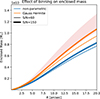 |
Fig. 11. Comparison of the estimated enclosed mass profile for NGC 4550 resulting from the Gauss Hermite (orange) and non-parametric (blue) stellar kinematics binned to different S/N. The thin lines show the result of the respective best-fit models seen so far with S/N = 60; the thick lines (and shaded uncertainty) show the results of the kinematic data binned to S/N = 150. |
This is again caused by an overestimation in σ. Binned to high S/N, this effect becomes stronger because, as more regions of the galaxy are binned together, the bimodal shapes of the respective LOSVDs become significantly smoothed out, especially so for the Gauss Hermite kinematic recoveries. Some of the bimodality is still resolved in the non-parametric kinematic data, leading to a smaller difference in the resulting mass estimate.
This is further supported by the orbit fractions and short axis tube distributions in Fig. 12. Interestingly, for both descriptions of stellar kinematics, the orbit fractions (upper panels) indicate a higher percentage of short axis tubes in comparison to the box orbits (again, the difference in the two binnings is more extreme for the Gauss Hermite kinematic data). This high fraction of short axis tubes at first seems counter-intuitive to the argument for higher dispersion in the high S/N case. However, the lower panels of Fig. 12 again show the distribution of the short axis tube orbits. On the bottom left, the distribution of the two non-parametric kinematic models are very similar, only showing a small preference for a dynamically warmer disk component at positive λz. For the Gauss Hermite case (bottom right), however, we find significantly warmer disks, suggesting higher σ of the tube orbits, in addition to the significant peak in box orbits in the inner regions of the galaxy (top right panel). Consequently, despite the higher fraction in short axis tubes, these are more dispersion-dominated, implying high dispersion and hence a higher mass.
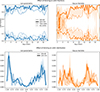 |
Fig. 12. Comparison of the differences caused by varying S/N in orbit fractions (upper panels, short axis-tubes: solid lines, box orbits: dashed lines) and circularity distributions (lower panels) for NGC 4550. Thick lines show results of S/N = 150 and the thin lines indicate previous results at S/N = 60 for comparison. Similarly to the difference in the estimated mass, the difference in the orbits caused by binning the kinematic data to different S/N is smaller for the non-parametric kinematic description. |
With Gauss Hermite, it appears to be more difficult to resolve kinematic substructure encoded in the observations, especially so when they are binned to higher S/N. The non-parametric kinematic recoveries are more robust to changes in spatial binning, both in terms of the LOSVD shape and subsequent dynamical inference.
We highlight that this investigation into the effect of the S/N concerns the choice of binning the signal of the data (which have been observed with a given S/N) to different values, resulting in a difference in the number and size of the resulting spatial bins. For modern observations resulting in higher S/N data, spatially binning to an accordingly high S/N does not result in such large spatial bins. Therefore, the bias we find for the Gauss Hermite models at different S/N binnings likely diminishes for more high-quality data.
For our cases, the significant differences in the Gauss Hermite solutions are likely caused by the bias term that induces regularisation in the kinematic extraction. This is not the case for our non-regularised non-parametric kinematic recovery. We also investigated how regularisation affects the results of the non-parametric kinematic data (in terms of the LOSVD shapes and the dynamical inferences). For details see Appendix D, but in short, we find a similarly large difference in the mass estimate as for Gauss Hermite, while the difference in the orbit distribution is smaller. This is because the bimodality resolved in the non-regularised LOSVDs gets smoothed out somewhat, being only noticeable in the most extreme cases of bimodality. This shows that a key question in terms of the kinematic extraction is how much regularisation is necessary.
6.4. Effect of uncertainty
Another aspect related to the recovery of the stellar kinematics between the parametric and non-parametric method is the observational uncertainty. In theory, the uncertainties of the kinematic data should be the same at every spatial bin, since the spectrum is binned to the same target S/N everywhere. In the outer regions of the galaxy, where the data are more affected by noise, the uncertainties may be slightly larger but not significantly so. Since the uncertainty of the kinematics informs how strongly the information from the individual spatial bins is weighted during the weight solving, we investigated the difference in the kinematic errors of NGC 2768.
The error for the non-parametric kinematics is directly inferred from the posterior sampling of the LOSVDs at each spatial bin. In order to compare the uncertainties across the galaxy, we summed over the logarithm of the uncertainties at each individual velocity bin at each spatial bin. Effectively, we then have one number quantifying the uncertainty in each region of the galaxy. For the non-parametric kinematic data, this is shown in the left panel of Fig. 13. We constructed the uncertainty map for the Gauss Hermite kinematics by following the same approach outlined in Sect. 3.3. We describe the LOSVD shape with the mean of the 500 LOSVDs sampled from the Gauss Hermite parameters and their errors. The uncertainties at each velocity bin (the same ones as for the non-parametric kinematics) were then taken as the 68% credibility interval from the range of sampled LOSVD shapes. We calculated the error in each spatial bin again by summing over the logarithm of each uncertainty value along all velocity bins. The Gauss Hermite uncertainty map is shown in the right panel of Fig. 13.
 |
Fig. 13. Uncertainty maps of the non-parametric (left) and Gauss Hermite (right) stellar kinematics for NGC 2768. |
It is immediately obvious that the uncertainties of the Gauss Hermite kinematics show a much stronger change from the inner to the outer regions than in the case of the non-parametric kinematics. While the latter shows a relatively flat uncertainty map (with the very centre regions only showing slightly smaller uncertainties), the Gauss Hermite uncertainty map shows very small values in the centre regions, significantly increasing outwards.
To investigate the effect of these differences in the kinematic uncertainties on the orbit distribution of our best-fit model, we performed a test where we adapt the Gauss Hermite errors so that the error map becomes flatter and similar to that of the non-parametric kinematic data. Naively, to achieve a spatially homogeneous uncertainties, one could try to set dv, dσ, dh3, and dh4 to constant values in every spatial bin. This, however, does not work, since even with constant dv, dσ, dh3, and dh4, the LOSVD uncertainty as we have defined it for the non-parametric case depends also depends on the values V, σ, h3, and h4, which are not spatially constant12. Therefore, we instead constructed a flat error map for the Gauss Hermite kinematics by multiplying the errors in h3 and h4 by ((rbin + α)/rbin, max)β, where rbin represents the radius at which the respective spatial bin is located, with α = 10 arcsec and β = −2. The right panel in Fig. 14 shows the adapted uncertainty map. We see that it is not completely flat in comparison to the left panel of Fig. 13 but it is the closest result to a flat error map we could construct with this approach. We then ran additional DYNAMITE models with these adapted kinematic datasets as input, fixing the hyper-parameters to the best-fit hyper-parameters from the original Gauss Hermite run. We note that in a thorough test of the impact of the uncertainties, it would be required to re-run the DYNAMITE models to select the new best-fit parameters, as they are also directly impacted by the measurement uncertainties. For the purpose of the current work, we are only interested in seeing their impact on the orbit distribution even at a fixed set of parameters.
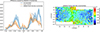 |
Fig. 14. Circularity distributions for NGC 2768 (left panel). The orange line shows the result of the original Gauss Hermite run; the grey line results from the adapted uncertainty map shown in the right panel. |
The left panel of Fig. 14 shows the impact of flattening the uncertainty map on the inferred λz distributions of the short axis tube orbits. We find notable changes with the peak λz value with changes in the uncertainty maps. It is not necessarily the case that the orbit distribution becomes more similar to that of the non-parametric results at increasingly flatter maps, but it is clear that a change in the uncertainties also leads to a change in the resulting dynamical model, even if the hyper-parameters are the same. It is therefore essential to have robust uncertainties associated with the stellar kinematics. Figure 13 suggests that the non-parametric recovery yields uncertainties that are more in line with expectations.
6.5. Limitations of Bayses-LOSVD
For the reasons discussed above, we infer that the non-parametric stellar kinematics extracted with Bayes-LOSVD yield more robust results in the dynamical inference in terms of information contained within the stellar LOSVD used as kinematic input. Specifically, we argue for an improvement in the constraints on the lower boundary of the total mass of galaxies due to making full use of the LOSVD information rather than relying on just the Gauss Hermite parameters. This is especially crucial for galaxies with complex kinematic substructures, which may have unrealistic values in σ and the higher-order moments. Even for regular galaxies, we find that the orbit fractions and distributions are affected by the choice of stellar kinematics. However, we note that, in the case of regular rotator NGC 2768, we also find seemingly spurious double-peaked signals with the non-parametric kinematics (Fig. B.6). This is one indication of how Bayes-LOSVD still faces some limitations. We have already mentioned the question of how much regularisation is necessary for the kinematic extraction from the spectra. While the non-regularised non-parametric stellar kinematics already show promising results in more robust constraints in the dynamical inference, the choice of the regularisation scheme will most likely limit the amount of dynamically cold orbits. This may be slightly overestimated in the current application, as the LOSVD shapes can be spiky, resulting in sudden drops in the LOSVD. This spikiness may also lead to the spurious double-peaked signals detected in the bimodality maps. While the non-regularised case can already be improved by decreasing the size of the velocity bins (Falcón-Barroso & Martig 2021), it will be imperative to find a (physically motivated) form of regularisation to avoid meaningless multiple peak detection. For the counter-rotating galaxy NGC 4550, the non-parametric bimodality map (upper right panel of Fig. 4) indicates double peaks that are spatially coherent and agree with the location of the counter-rotating disks in the middle left panel of Fig. 1. As we find more significant differences – especially concerning the estimated total mass – for this galaxy than for NGC 2768, we tentatively conclude that even with some spurious detection of bimodal features, the non-regularised non-parametric kinematics method yields similar results as the parametric method, while we find more robust results for a galaxy with complex kinematics, as the signal from any coherent kinematic substructures outweighs the influence of non-physical spikes caused by the lack of regularisation.
At this point, it is also necessary to point out the longer computational time required for the posterior sampling. While the kinematic extraction with pPXF for more than a thousand spatial bins is done within minutes, this requires several hours for Bayes-LOSVD, even when the kinematic extraction is performed at several spatial bins in parallel. This problem increases at finer spatial binning and velocity sampling due to the higher number of parameters. However, it is important to keep in mind that from this posterior sampling, we also directly get a robust uncertainty estimate. With pPXF, the MC sampling for the error estimation still needs to be done after the kinematic inference, increasing the computing tine by a factor of 10.
In Sect. 3.3, we have mentioned the issue of sudden spikes in the outer velocity bins in some of the outer spatial bins (see bottom right panel of Fig. 4). This corresponds to the regions with the lowest S/N spectra. In order to avoid problems with the dynamical inference in these regions, we manually modified the uncertainties in these regions to be larger. This, in turn, reduces the impact of the affected velocity bins on the dynamical modelling. However, this also means that any information contained in the LOSVD tails of these regions is not taken into account. In Mehrgan et al. (2019), the authors point out that the LOSVD tails constrain the escape velocity and, in turn, the potential of the galaxy. As our increased uncertainties in some of the wings may therefore suppress the tails, it may happen that we underestimate the mass. However, since the mass estimate for NGC 2768 is similar for both types of stellar kinematics, we do not expect the tail regions to significantly affect our findings for NGC 4550. It will nevertheless be important in the future to find a solution for avoiding these sudden spikes in the tails. Once again, we expect that this issue should be significantly improved by the implementation of a more informed prior for regularisation. In addition, we expect higher S/N data to be less affected by these spikes in the tails, as they mainly appear in regions of low S/N.
7. Conclusions and outlook
We investigated the difference in the results of orbit-superposition models using two types of kinematic input: a parametric LOSVD based on Gauss Hermite expansion extracted from the spectrum using pPXF and a non-parametric description of the LOSVD recovered using a Bayesian framework, Bayes-LOSVD. This was applied to the datacubes of NGC 4550, which contains two counter-rotating disks, and regular rotator NGC 2768. We explored the resulting hyper-parameter space and analysed the mass, shape and anisotropy profiles, and the orbit distributions resulting from the respective best fitting models. The main findings are:
-
Based solely on the kinematics, we recover a bimodal structure of the LOSVD for NGC 4550 in the non-parametric framework, suggesting counter-rotation. This is not the case for the kinematic extraction using Gauss Hermite parametrisation, which overall results in broad unimodal LOSVDs. In turn, this leads to a larger σ than might have been expected (Fig. 4) based on the non-parametric result. A higher σ implies a higher predicted dispersion for the orbits in the dynamical models. The LOSVDs of regular rotator NGC 2768 are more similar, as the LOSVDs are mainly Gaussian in both recoveries. In the non-parametric recovery, we find some indication of additional kinematic substructures.
-
Due to the larger dispersion, the total mass of NGC 4550 is notably higher in the Gauss Hermite-based models (Fig. 5). From the comparison with Cappellari et al. (2007), we suggest that this has also been the case in previous models using Gauss Hermite kinematic recoveries as input. There is no significant difference in the mass estimates of NGC 2768.
-
We find that both the shape and anisotropy profiles suggest a thinner, more rotation-dominated structure for both galaxies using the non-parametric kinematic recoveries (Figs. 6 and 7).
-
The non-parametric kinematic input results in two distinct dynamically cold peaks at λz ± 1 for NGC 4550 with a high fraction of short axis tubes (Fig. 9). The Gauss Hermite models result in 15% fewer tube orbits and twice as many box orbits, which is likely what causes the difference in the mass, shape, and anisotropy profiles. We find a similar but less significant trend in the orbit fractions for NGC 2768. Here, the non-parametric models again suggest less triaxial and less radially dominated orbits caused by the slightly lower fraction of box orbits and a more dynamically warm disk.
-
We find that the non-parametric kinematic recoveries are more similar at different spatial binnings and more robust in terms of their uncertainties (Figs. 12 and 13, respectively). In addition, they avoid the issue of choosing between fit metrics.
While it has been known that parametric descriptions of the LOSVD cannot capture the full complexity of kinematics found in both observations and numerical simulations, this work highlights the consequences in dynamical inference. Due to the discrepancy in the shape and anisotropy profile, as well as in the orbit distribution and, in the most extreme case of NGC 4550 also in the estimated mass, we suggest moving towards non-parametric kinematic recoveries. This will be especially important for the analysis of high-resolution spectra, for example from future surveys such as Hector (Bryant et al. 2024) and BlueMUSE (Richard et al. 2024), and for high-z spectroscopy with HARMONI (Thatte et al. 2016). Non-parametric kinematic recoveries will be more sensitive to the detection of kinematic substructures. The ability to resolve these substructures will allow us to make better use of the potential of the data.
An open question in the extraction of non-parametric kinematics from spectra is the amount of regularisation that is required in the inference. Current regularisation techniques in Bayes-LOSVD can smoothen out bimodal LOSVDs, resulting in broader velocity distributions and hence a higher fraction of dispersion-dominated orbits, making the regularised Bayes-LOSVD results more similar to the Gauss Hermite solution. To make full use of the advantages of the non-parametric kinematics, it will be imperative to find a physically motivated form of regularisation, which smoothens out any spurious bimodal detections from spiky LOSVD shapes, while keeping them flexible enough to detect spatially coherent multi-peak signals.
This question of regularisation also concerns the dynamical inference itself. In this work, we have indicated uncertainties in the dynamical models by a range of 50 models that fit the data well. However, in order to properly compare differences in orbit distributions, an improvement in the uncertainty quantification will be necessary to differentiate between distinct dynamical substructures. Similar to the question of regularisation in the kinematic recovery, it will be necessary to implement a more informed prior in the orbit computation. A potential approach for this is to use the information from cosmological simulations to construct a Bayesian prior for the orbit solution, similar to Remy et al. (2023), who used deep learning of priors in the context of weak lensing. This is subject to ongoing study. An additional idea we are planning on investigating is to use cosmological simulation to also create mock observations, which can be used with Bayes-LOSVD to analyse the impact of variation in the LOSVD tails, as well as any potential overestimation of the dynamically cold components resulting from the non-parametric kinematics.
The table for all galaxies is given in the section entitled ‘MGE parameters for the deconvolved r-band surface brightness’ at http://www-astro.physics.ox.ac.uk/atlas3d/
The authors thank Jesús Falcón-Barroso for initially providing the datacube in the form that was used in the tests for Bayes-LOSVD in Falcón-Barroso & Martig (2021).
The velocity bins are not symmetric around 0 due to our choice of a bin width of 60 km s−1. While we manually set a velocity range of [ − 700, 700] km s−1, Bayes-LOSVD automatically adapts the velocity range to [ − 667, 712] to be divisible by 60.
The intrinsic shape parameters indicate the triaxiality of the system, for more details see Cappellari (2002), van den Bosch et al. (2008).
This dark matter profile is derived from the mass-dependent halo concentration taken from the simulations detailed in Navarro et al. (1996). This is done as the SAURON data constrain only the inner regions of galaxies, providing little to no constraints on their dark matter component.
We tested whether our findings change when using a larger orbit library, but find no differences in the goodness-of-fit.
We performed the deprojection using the intrinsic shape parameters resulting from the Gauss Hermite kinematics.
The separation into the two disks can be done similarly with the Gauss Hermite model result but we highlight that setting the cut at λz = ±0.75 yields a lower fraction of total orbit weights in these regions due to the counter-rotating peak being shifted to lower |λz|, in turn resulting in less massive disk components.
The reason for choosing NGC 2768 here as an example rather than NGC 4550 is that the Gauss Hermite uncertainty map of the counter-rotating galaxy is more complex. The non-parametric uncertainty map is again flat, while the Gauss Hermite uncertainties show systematic differences between the counter-rotating and non-counter-rotating regions. It would therefore require more fine-tuning to modify the Gauss Hermite map, which would go beyond the scope of this paper.
High spectral resolution is necessary to properly constrain higher-order Gauss Hermite moments. Additionally, these higher-order moments do not have an easily interpretable meaning for the distribution as h3 and h4 do (skewness and curtosis, respectively).
Acknowledgments
This research was funded by the Austrian Science Fund (FWF) SFB 10.55776/F68 “Tomography Across the Scales”, project F6811- N36 (Advancing Extragalactic Archeology through Novel Inversion Techniques). The computational results presented have been achieved [in part] using the Vienna Scientific Cluster (VSC). The authors thank the referee for their valuable input and their many suggestions to improve this manuscript. The authors thank Alice Zocchi for her valuable comments and discussion points in the preparation of this manuscript.
References
- Bacon, R., Adam, G., Baranne, A., et al. 1995, A&AS, 113, 347 [NASA ADS] [Google Scholar]
- Binney, J., & Tremaine, S. 1987, Galactic Dynamics (Princeton: Princeton University Press) [Google Scholar]
- Bro, R., & De Jong, S. 1997, J. Chemom., 11, 393 [CrossRef] [Google Scholar]
- Bryant, J. J., Oh, S., Gunawardhana, M., et al. 2024, SPIE Conf. Ser., 13096, 130960D [Google Scholar]
- Bundy, K., Bershady, M. A., Law, D. R., et al. 2015, ApJ, 798, 7 [Google Scholar]
- Cappellari, M. 2002, MNRAS, 333, 400 [NASA ADS] [CrossRef] [Google Scholar]
- Cappellari, M. 2008, MNRAS, 390, 71 [NASA ADS] [CrossRef] [Google Scholar]
- Cappellari, M. 2017, MNRAS, 466, 798 [Google Scholar]
- Cappellari, M., & Emsellem, E. 2004, PASP, 116, 138 [Google Scholar]
- Cappellari, M., Bacon, R., Bureau, M., et al. 2006, MNRAS, 366, 1126 [Google Scholar]
- Cappellari, M., Emsellem, E., Bacon, R., et al. 2007, MNRAS, 379, 418 [Google Scholar]
- Cappellari, M., Emsellem, E., Krajnović, D., et al. 2011, MNRAS, 413, 813 [Google Scholar]
- Coccato, L., Morelli, L., Pizzella, A., et al. 2013, A&A, 549, A3 [Google Scholar]
- Croom, S. M., Lawrence, J. S., Bland-Hawthorn, J., et al. 2012, MNRAS, 421, 872 [NASA ADS] [Google Scholar]
- Deason, A. J., & Belokurov, V. 2024, New Astron. Rev., 99, 101706 [CrossRef] [Google Scholar]
- Derkenne, C., McDermid, R. M., Santucci, G., et al. 2024, MNRAS, 533, 1300 [Google Scholar]
- Ding, Y., Zhu, L., van de Ven, G., et al. 2023, A&A, 672, A84 [NASA ADS] [CrossRef] [EDP Sciences] [Google Scholar]
- Emsellem, E., Monnet, G., & Bacon, R. 1994, A&A, 285, 723 [NASA ADS] [Google Scholar]
- Emsellem, E., Cappellari, M., Peletier, R. F., et al. 2004, MNRAS, 352, 721 [Google Scholar]
- Emsellem, E., Cappellari, M., Krajnović, D., et al. 2007, MNRAS, 379, 401 [Google Scholar]
- Falcón-Barroso, J., & Martig, M. 2021, A&A, 646, A31 [NASA ADS] [CrossRef] [EDP Sciences] [Google Scholar]
- Forbes, D. A., Cortesi, A., Pota, V., et al. 2012, MNRAS, 426, 975 [CrossRef] [Google Scholar]
- Foster, C., Mendel, J. T., Lagos, C. D. P., et al. 2021, PASA, 38, e031 [NASA ADS] [CrossRef] [Google Scholar]
- Gaia Collaboration (Prusti, T., et al.) 2016, A&A, 595, A1 [NASA ADS] [CrossRef] [EDP Sciences] [Google Scholar]
- Gasymov, D., & Katkov, I. 2024, ASP Conf. Ser., 535, 279 [Google Scholar]
- Gelman, A., & Rubin, D. B. 1992, Stat. Sci., 7, 457 [Google Scholar]
- Gerhard, O. E. 1993, MNRAS, 265, 213 [Google Scholar]
- Jethwa, P., Thater, S., Maindl, T., & Van de Ven, G. 2020, Astrophysics Source Code Library [record ascl:2011.007] [Google Scholar]
- Johnston, E. J., Merrifield, M. R., Aragón-Salamanca, A., & Cappellari, M. 2013, MNRAS, 428, 1296 [Google Scholar]
- Lawson, C. L., & Hanson, R. J. 1995, Solving Least Squares Problems (Society for Industrial and Applied Mathematics) [Google Scholar]
- Long, R. J., & Mao, S. 2012, MNRAS, 421, 2580 [Google Scholar]
- Loubser, S. I., Hoekstra, H., Babul, A., & O’Sullivan, E. 2018, MNRAS, 477, 335 [NASA ADS] [CrossRef] [Google Scholar]
- McDermid, R. M., Emsellem, E., Shapiro, K. L., et al. 2006, MNRAS, 373, 906 [Google Scholar]
- Mehrgan, K., Thomas, J., Saglia, R., et al. 2019, ApJ, 887, 195 [NASA ADS] [CrossRef] [Google Scholar]
- Mehrgan, K., Thomas, J., Saglia, R., Parikh, T., & Bender, R. 2023, ApJ, 948, 79 [NASA ADS] [CrossRef] [Google Scholar]
- Nakashima, J.-I., Koning, N., Kwok, S., & Zhang, Y. 2009, ApJ, 692, 402 [Google Scholar]
- Navarro, J. F., Frenk, C. S., & White, S. D. M. 1996, ApJ, 462, 563 [Google Scholar]
- Poci, A., McDermid, R. M., Lyubenova, M., et al. 2021, A&A, 647, A145 [NASA ADS] [CrossRef] [EDP Sciences] [Google Scholar]
- Poci, A., McDermid, R. M., Lyubenova, M., et al. 2022, MNRAS, 514, 3660 [NASA ADS] [CrossRef] [Google Scholar]
- Remy, B., Lanusse, F., Jeffrey, N., et al. 2023, A&A, 672, A51 [NASA ADS] [CrossRef] [EDP Sciences] [Google Scholar]
- Rich, R. M., Mosenkov, A., Lee-Saunders, H., et al. 2019, MNRAS, 490, 1539 [Google Scholar]
- Richard, J., Giroud, R., Laurent, F., et al. 2024, SPIE Conf. Ser., 13096, 1309622 [Google Scholar]
- Rix, H.-W., Franx, M., Fisher, D., & Illingworth, G. 1992, ApJ, 400, L5 [NASA ADS] [CrossRef] [Google Scholar]
- Roy, V. 2020, Annu. Rev. Stat. Appl., 7, 387 [Google Scholar]
- Rubin, V. C., Graham, J. A., & Kenney, J. D. P. 1992, ApJ, 394, L9 [NASA ADS] [CrossRef] [Google Scholar]
- Rubino, M., Pizzella, A., Morelli, L., et al. 2021, A&A, 654, A30 [NASA ADS] [CrossRef] [EDP Sciences] [Google Scholar]
- Saha, P., & Williams, T. B. 1994, AJ, 107, 1295 [Google Scholar]
- Sánchez, S. F., Kennicutt, R. C., Gil de Paz, A., et al. 2012, A&A, 538, A8 [Google Scholar]
- Sanders, J. L., & Evans, N. W. 2020, MNRAS, 499, 5806 [Google Scholar]
- Santucci, G., Brough, S., van de Sande, J., et al. 2022, ApJ, 930, 153 [NASA ADS] [CrossRef] [Google Scholar]
- Santucci, G., Lagos, C. D. P., Harborne, K. E., et al. 2024, MNRAS, 534, 502 [Google Scholar]
- Schwarzschild, M. 1979, ApJ, 232, 236 [NASA ADS] [CrossRef] [Google Scholar]
- Schwarzschild, M. 1982, ApJ, 263, 599 [NASA ADS] [CrossRef] [Google Scholar]
- Scott, N., Cappellari, M., Davies, R. L., et al. 2013, MNRAS, 432, 1894 [NASA ADS] [CrossRef] [Google Scholar]
- Shetty, S., Bershady, M. A., Westfall, K. B., et al. 2020, ApJ, 901, 101 [CrossRef] [Google Scholar]
- Syer, D., & Tremaine, S. 1996, MNRAS, 282, 223 [Google Scholar]
- Thater, S., Jethwa, P., Lilley, E. J., et al. 2023, IAU Symp. Proc. Ser., 379 [Google Scholar]
- Thatte, N. A., Clarke, F., Bryson, I., et al. 2016, SPIE Conf. Ser., 9908, 99081X [NASA ADS] [Google Scholar]
- Urrutia, T., Wisotzki, L., Kerutt, J., et al. 2019, A&A, 624, A141 [NASA ADS] [CrossRef] [EDP Sciences] [Google Scholar]
- van de Ven, G., de Zeeuw, P. T., & van den Bosch, R. C. E. 2008, MNRAS, 385, 614 [NASA ADS] [CrossRef] [Google Scholar]
- van den Bosch, R. C. E., van de Ven, G., Verolme, E. K., Cappellari, M., & de Zeeuw, P. T. 2008, MNRAS, 385, 647 [Google Scholar]
- van der Marel, R. P., & Franx, M. 1993, ApJ, 407, 525 [Google Scholar]
- Vazdekis, A. 1999, ApJ, 513, 224 [NASA ADS] [CrossRef] [Google Scholar]
- Vazdekis, A., Coelho, P., Cassisi, S., et al. 2015, MNRAS, 449, 1177 [Google Scholar]
- Weijmans, A.-M., Krajnović, D., van de Ven, G., et al. 2008, MNRAS, 383, 1343 [Google Scholar]
- Zhu, L., van den Bosch, R., van de Ven, G., et al. 2018, MNRAS, 473, 3000 [Google Scholar]
- Zhu, L., van de Ven, G., Leaman, R., et al. 2022, A&A, 664, A115 [NASA ADS] [CrossRef] [EDP Sciences] [Google Scholar]
Appendix A: Higher-order Gauss Hermite and adapted kinematics
We also recovered the Gauss Hermite parameters up to order six (case 1) and to order eight (case 2), to investigate the difference in these parametric stellar kinematics with the non-parametric stellar kinematics in NGC 4550.13 We find that even at higher-order moments, the bimodal shapes of the LOSVDs are generally not resolved but there is a clear shift to one of the two peaks recovered with the non-parametric kinematics. This effectively reduces the σ estimate slightly. However, due to the stronger deviations from a regular Gaussian shape, the contribution of negative values in the LOSVD increase, especially so at order eight. This is an unphysical result, as it implies negative light contribution. For this reason, we only use the order six stellar kinematics for subsequent dynamical modelling.
The dynamical inference with Gauss Hermite sixth-order stellar kinematics results in a mass estimate between the Gauss Hermite fourth-order and the non-parametric kinematic data. The orbit distribution of the short axis tubes is, however, still dominated by dynamically warm orbits. We therefore note that simply moving to higher orders in the Gauss Hermite expansion slightly reduces the disparity in the mass estimate but not in the overall discrepancy in the orbit distribution, as the bimodal LOSVDs are still not resolved in the higher-order parametric kinematics.
To further analyse the difference between Gauss Hermite and the non-parametric kinematics, we also tested what happens when we set boundaries on σ in pPXF via the bounds-variable. The main aim of this approach is to see whether the results of the dynamical models become more similar to those of the non-parametric kinematics, if we force the parametric description to resemble it as closely as possible. We tested different values for the minimum and maximum in σ and compared the results to those of the non-parametric LOSVDs. We find the smallest difference between the two cases for a σ between 70 km s−1 ≤ σ ≤ 85 km s−1 in the counter-rotating regions. An example of this modified parametric LOSVD is shown in Fig. A.1.
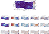 |
Fig. A.1. Difference of the LOSVD shapes for a different parametrisation. Moments up to order six with limits on σ. The non-parametric and the unmodified Gauss Hermite LOSVDs are shown for comparison. |
An issue of these bounds, however, is that the MC sampling for the error estimation now no longer leads to a normal distribution of values but rather a pile-up at the two boundary values. To avoid this issue where possible, we created our final modified parametric kinematic dataset as a mix of the two approaches: for the spatial bins containing bimodal LOSVDs (identified from the non-parametric kinematics), we set the bounds on σ, while in every other case we did not. We used Gauss Hermite moments up to order six.
The modified model with bounds on σ yield a significantly lower mass estimate than the regular Gauss Hermite case. This is as expected, as the bounds on σ limit the dispersion and hence reduce the recovered total mass of the galaxy. Interestingly however, we find an even lower mass estimate than for the non-parametric kinematic data. This indicates that the bounds on σ are likely too limiting. The galaxy model from this modified Gauss Hermite fit has a smaller fraction of box orbits than in the original Gauss Hermite model, making the result slightly more similar to that of the non-parametric kinematic data.
We have done these tests to investigate how sensitive the dynamical modelling is to changes in the kinematic input data and how sensitive the Gauss Hermite expansion is to changes in the pPXF settings. However, we note that such artificial modification of the parametric kinematic extraction is not useful in practice. This is because, even in the modified case, we still do not fully recover the bimodal LOSVD shapes properly and in reality we have no reference for such boundary conditions on σ.
Appendix B: Goodness-of-fit: Kinematics and dynamical modelling
Here we discuss the goodness-of-fit in both the stellar kinematics and the dynamical modelling, respectively. Figure B.1 shows the h3 (upper panels) and h4 (lower panels) kinematic maps of NGC 4550 (left) and NGC 2768 (right), similar to the v/σ maps in Fig. 1.
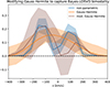 |
Fig. B.1. Moment maps (top row = h3, bottom row = h4) of NGC 4550 (left) and NGC 2768 (right). |
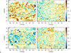 |
Fig. B.2. Spectrum fits for NGC 4550 and 2768 for the non-regularised fits with Bayes-LOSVD. The four individual spectra correspond to the four regions noted in Figs. 4 and B.6 in descending order. The grey regions define the masked regions during the spectral fit. |
To indicate how well the kinematic models fit the data in Bayes-LOSVD, Fig. B.2 shows the spectrum fits for the four spatial regions highlighted in Fig. 4 (numbers are in descending order). As we have used the Gauss Hermite kinematics from Emsellem et al. (2004), we cannot show the spectrum fit from pPXF but we highlight that Fig. B2 from their work shows example spectrum fits in a similar way to our Fig. B.2 for comparison. In the left panel of this figure, the bottom spectrum is one example for the fit in an outermost spatial bin, where we also find a spike at the negative velocity tail.
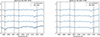 |
Fig. B.3. As in Fig. 4, but for NGC 4550 binned to high S/N. The upper right panel shows the spectrum fits for both the non-parametric and the Gauss Hermite kinematics in the four indicated regions. |
To illustrate the difference in the spectrum fits for Bayes-LOSVD and pPXF, Fig. B.3, shows the bimodality map for NGC 4550 binned to high S/N (i.e. fewer spatial bins) on the top left and the spectrum fits corresponding to the example regions on the top right panel. As discussed in Sect. 6.3, for this case we have re-run pPXF with our spatial binning, so we are also showing the four example spectrum fits from this method. Except for the bottom spectrum (corresponding to region 4), the two methods can fit the data equally well. As in the left panel of Fig. B.2, we see larger differences between the observed spectrum and the spectrum fit in this case. The bottom four panels of Fig. B.3 show the recovered LOSVDs from the spectrum fits. We find similar differences as discussed in Sect. 3.
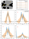 |
Fig. B.4. Local χ2 map for the non-parametric (top panel, Ndof = Nvelocity − bins) and residual maps for the Gauss Hermite (bottom panels) dynamical model for NGC 4550. |
To evaluate the goodness-of-fit of the dynamical models, Figs. B.4 and B.5 show the χ2 maps (top panels) of the non-parametric and the residual maps (lower panels) of the Gauss Hermite best-fit models for NGC 4550 and NGC 2768, respectively. We point out that the χ2 values of the non-parametric models can be < 1 because of the overestimation of the kinematic uncertainty. Nevertheless, the χ2 values are comparable between the spatial bins. Additionally, the lower four panels of Fig. 10 shows some example model LOSVDs in four different regions for NGC 4550. Both visualisations (Figs. 10 and B.4) indicate a good fit of the model with the data except in some of the outer bins, where the spikes appear in the velocity tails. The residual maps from the best-fit Gauss Hermite model similarly shows a good fit to the data and, in the model velocity map, the counter-rotation is well-resolved.
For NGC 2768, the non-parametric dynamical model indicates very good agreement with the data in most regions (upper panel of Fig. B.5), except for some seemingly random spatial bins, where the difference between data and model is comparatively large. Comparing the χ2 map to the bimodality map of the non-parametric NGC 2768 in the top right panel of Fig. B.6 indicates that the high χ2 values at least partially overlap with the spurious double-peak detections. Similarly, the residual maps from the Gauss Hermite best-fit dynamical model (lower panels of Fig. B.5) show relatively low values. We therefore conclude that both models fit comparatively well with the data (with respect to the kinematic uncertainties).
The lower panels of Fig. B.6 show four examples of what the non-parametric and Gauss Hermite LOSVDs look like in regions where we pick up multiple peaks in the non-parametric LOSVD. Due to the random distribution of double peaks detected in the upper right panel of this Figure, it is likely that Bayes-LOSVD is picking up noise in the data, resulting in the less smooth LOSVD shapes. As the resulting dynamical models are comparable for the non-parametric and Gauss Hermite case for NGC 2768 (compare Figs. 5, 8, 9, and B.5), we argue that the dynamical models are not as sensitive to this noise (likely because of the large uncertainties) as they are to spatially coherent multi-peak signal as in NGC 4550 (Figs. 4 and B.3). Nevertheless, we reiterate the importance of looking for more informed regularisation to differentiate real kinematic substructure and random noise in the spectrum fit.
Appendix C: Choice of fit metric
As discussed in Sect. 4, the dynamical inference based in the Gauss Hermite kinematics results in two metrics, on which the best-fit model can be selected, χkin2 and χkinmap2. For the non-parametric kinematic input, the weight solving yields only one fit metric.
Figure C.1 shows the differences in the mass profile (left panel), the orbit fractions (middle panel), and the orbit distribution of the short axis tubes (right panel) for NGC 4550. The orange lines show our results presented in the main text (that is, based on χkinmap2) and the red line the best-fit model (and related uncertainty) based on χkin2. Based on the uncertainty range – given by the range of 50 best-fit models – the model selection does seem to overlap significantly for both fit metrics. We note that in the set-up for the dynamical modelling, we set the which_chi-parameter, based on which the grid search proceeds, to χkinmap2. The range of models might change slightly if we search based on χkin2 instead.
The left panel of Fig. C.1 shows that the total mass estimate for the χkin2 models is even larger than the χkinmap2 estimate. In comparison to the orbit fractions, this seems counter-intuitive, as the fraction of box orbits is significantly higher in the χkinmap2-selected models, which would indicate a higher dispersion. However, the orbit distribution shows that the distribution of short axis tubes is similar for both best-fit models, with the exception that the surplus of short axis tubes in the χkin2-selected models has an average λz of 0.35. This contributes significantly to higher overall σ. We note that when binned to higher S/N, the differences caused by the χ2-selection increase significantly.
Figure C.2 shows the same comparison for regular rotator NGC 2768. We find similar – but significantly weaker – effects in the mass, orbit fractions, and orbit distributions as explained for NGC 4550. The differences caused by the choice of fit metric for regular rotating galaxies seem to be negligible. As Fig. C.1 has shown, this is not the case for galaxies with more complex kinematics. As it is not immediately obvious which metric is the better choice, moving towards the non-parametric modelling with straightforward χ2-minimisation may be the preferable option.
Appendix D: Regularisation in Bayes-LOSVD
As a short overview, the current regularisation schemes implemented in Bayes-LOSVD are the non-regularised case (assuming independent, identical priors for all velocity bins), the random-walk prior (where neighbouring velocity bins are linked), the auto-regressive prior with adjustable settings (linking more velocity bins depending on the order), and penalised B-splines (which link the spline coefficients rather than the velocity bins). For a more detailed explanation on the individual options, see Falcón-Barroso & Martig (2021).
While the non-regularised method yields larger uncertainties, the results are not biased towards smoother solutions. It is therefore possible to recover more complex structures. As pointed out in Falcón-Barroso & Martig (2021), NGC 4550 is an example for the caution necessary when implementing regularisation in the kinematic extraction.
For our study of NGC 4550 and NGC 2768, we used the non-regularised scheme for the recovery of the stellar kinematics with Bayes-LOSVD. To investigate the impact of adding some level of regularisation in the stellar kinematics on the dynamical inference, we also construct a non-parametric kinematic dataset using the auto-regressive prior of order 3. In the LOSVD shapes, we find that they are more similar to the Gauss Hermite LOSVDs, as they are largely unimodal in the regions where the non-regularised approach has resolved the bimodality in the velocity distribution.
To test whether this, as we expected, leads to a difference in the dynamical models as well, we also used the regularised kinematic datasets for NGC 4550 and NGC 2768 in the dynamical modelling. The results are shown in Fig. D.1 for NGC 4550. Similar to the difference caused by the choice of fit metric in App. C, the same trends can also be found for NGC 2768 but on a significantly smaller scale.
The left panel of Fig. D.1 shows the total mass estimate. Interestingly, the total mass inferred from the regularised case is even higher than in the Gauss Hermite case, although both lie within the error bars of each other. Generally, we find that the range of possible models covers a large range in mass for the regularised non-parametric kinematics. It even includes the non-regularised mass estimate, which is lower by almost 0.5 dex.
The middle and right panels of Fig. D.1 show the orbit fraction and distribution of NGC 4550, respectively. Overall the orbit fraction profiles are more similar to those of the non-regularised non-parametric kinematics. Only at around 3.5 arcsec does the fraction of box orbits of the regularised kinematic input show the same sudden spike as in the Gauss Hermite models, suggesting central regions with high velocity-dispersions. The distribution of the high number of short axis tube orbits shows the same distribution as that of the Gauss Hermite short axis tubes, peaking at smaller |λz| than the non-regularised non-parametric models. Again, this is likely the reason for the higher mass estimate we find in the left panel.
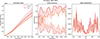 |
Fig. D.1. Difference in enclosed mass profiles (left), orbit fraction (middle), and the orbit distribution (right) of NGC 4550 between the χkinmap2-selected and χkin2-selected best-fit models (orange and red lines, respectively). |
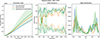 |
Fig. D.3. Comparison of the best-fit mass (left), orbit fractions (middle), and distribution of the short axis tube orbits (right) of NGC 4550 resulting from the non-regularised and regularised non-parametric kinematics (blue and green lines, respectively) and the Gauss Hermite kinematics (orange). |
All Tables
DYNAMITE runs performed with the respective kinematic input for NGC 4550 and NGC 2768.
Comparison of global values for the best-fit parameters, velocity anisotropy parameters, and relative contributions of different orbit types of NGC 4550.
All Figures
|
Fig. 1. Surface brightness contours (upper panels) of NGC 4550 (left) and NGC 2768 (right). The middle and lower panels show the v/σ maps constructed with the Gauss Hermite and non-parametric kinematics, respectively. |
| In the text | |
|
Fig. 2. Channel maps constructed from the non-parametric stellar kinematics of NGC 4550 over all spatial bins in different velocity intervals. The percentage of the contribution of each spatial bin to the specified velocity bin is colour-coded (see colour bar at right). |
| In the text | |
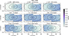 |
Fig. 3. As in Fig. 2, but for NGC 2768. |
| In the text | |
|
Fig. 4. Bimodality maps (upper panels) of NGC 4550 and comparison of different Gauss Hermite and non-parametric LOSVD shapes for four example spatial bins. |
| In the text | |
|
Fig. 5. Enclosed mass profiles for NGC 4550 (left) and NGC 2768 (right) resulting from Gauss Hermite parametrisation (orange) and the non-parametric description of the kinematics (blue). For NGC 4550, the comparison includes the results of Cappellari et al. (2006) (solid line) and Long & Mao (2012) (dashed line). |
| In the text | |
|
Fig. 6. Shape profiles of NGC 4550 (left) and NGC 2768 (right), where p (dotted line) and q (dashed line) are two axis ratios and T (solid line) gives the triaxiality of the galaxy. For both galaxies, the difference between the two methods is most apparent in p, which translates into T. |
| In the text | |
|
Fig. 7. Spherical (upper row) and cylindrical (bottom row) velocity anisotropy profiles of NGC 4550 (left column) and NGC 2768 (right column) resulting from the dynamical models using the Gauss Hermite kinematics (orange) and the non-parametric kinematics (blue), respectively. |
| In the text | |
|
Fig. 8. Relative orbit fractions for the short axis tubes (solid lines) and the box orbits (dashed lines) from the Bayes-LOSVD (blue) and Gauss Hermite (orange) models, respectively, for NGC 4550 (left) and NGC 2768 (right). |
| In the text | |
|
Fig. 9. One-dimensional circularity distribution of the short axis tube orbits of NGC 4550 (left) and NGC 2768 (right) resulting from the non-parametric (blue) and the parametric (orange) kinematics. |
| In the text | |
|
Fig. 10. As in Fig. 4, but the top left panel shows the bimodality map of the best-fit model of NGC 4550. The middle and bottom panels show the LOSVDs of the data (solid lines) and the model (dashed lines) of the same spatial bins as in Fig. 4. |
| In the text | |
|
Fig. 11. Comparison of the estimated enclosed mass profile for NGC 4550 resulting from the Gauss Hermite (orange) and non-parametric (blue) stellar kinematics binned to different S/N. The thin lines show the result of the respective best-fit models seen so far with S/N = 60; the thick lines (and shaded uncertainty) show the results of the kinematic data binned to S/N = 150. |
| In the text | |
|
Fig. 12. Comparison of the differences caused by varying S/N in orbit fractions (upper panels, short axis-tubes: solid lines, box orbits: dashed lines) and circularity distributions (lower panels) for NGC 4550. Thick lines show results of S/N = 150 and the thin lines indicate previous results at S/N = 60 for comparison. Similarly to the difference in the estimated mass, the difference in the orbits caused by binning the kinematic data to different S/N is smaller for the non-parametric kinematic description. |
| In the text | |
|
Fig. 13. Uncertainty maps of the non-parametric (left) and Gauss Hermite (right) stellar kinematics for NGC 2768. |
| In the text | |
|
Fig. 14. Circularity distributions for NGC 2768 (left panel). The orange line shows the result of the original Gauss Hermite run; the grey line results from the adapted uncertainty map shown in the right panel. |
| In the text | |
|
Fig. A.1. Difference of the LOSVD shapes for a different parametrisation. Moments up to order six with limits on σ. The non-parametric and the unmodified Gauss Hermite LOSVDs are shown for comparison. |
| In the text | |
|
Fig. B.1. Moment maps (top row = h3, bottom row = h4) of NGC 4550 (left) and NGC 2768 (right). |
| In the text | |
|
Fig. B.2. Spectrum fits for NGC 4550 and 2768 for the non-regularised fits with Bayes-LOSVD. The four individual spectra correspond to the four regions noted in Figs. 4 and B.6 in descending order. The grey regions define the masked regions during the spectral fit. |
| In the text | |
|
Fig. B.3. As in Fig. 4, but for NGC 4550 binned to high S/N. The upper right panel shows the spectrum fits for both the non-parametric and the Gauss Hermite kinematics in the four indicated regions. |
| In the text | |
|
Fig. B.4. Local χ2 map for the non-parametric (top panel, Ndof = Nvelocity − bins) and residual maps for the Gauss Hermite (bottom panels) dynamical model for NGC 4550. |
| In the text | |
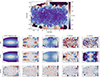 |
Fig. B.5. Same as Fig. B.4, but for NGC 2768. |
| In the text | |
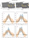 |
Fig. B.6. As in Fig. 4, but for NGC 2768. |
| In the text | |
|
Fig. D.1. Difference in enclosed mass profiles (left), orbit fraction (middle), and the orbit distribution (right) of NGC 4550 between the χkinmap2-selected and χkin2-selected best-fit models (orange and red lines, respectively). |
| In the text | |
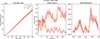 |
Fig. D.2. As in Fig. C.1, but for NGC 2768. |
| In the text | |
|
Fig. D.3. Comparison of the best-fit mass (left), orbit fractions (middle), and distribution of the short axis tube orbits (right) of NGC 4550 resulting from the non-regularised and regularised non-parametric kinematics (blue and green lines, respectively) and the Gauss Hermite kinematics (orange). |
| In the text | |
Current usage metrics show cumulative count of Article Views (full-text article views including HTML views, PDF and ePub downloads, according to the available data) and Abstracts Views on Vision4Press platform.
Data correspond to usage on the plateform after 2015. The current usage metrics is available 48-96 hours after online publication and is updated daily on week days.
Initial download of the metrics may take a while.