| Issue |
A&A
Volume 701, September 2025
|
|
|---|---|---|
| Article Number | A81 | |
| Number of page(s) | 15 | |
| Section | Numerical methods and codes | |
| DOI | https://doi.org/10.1051/0004-6361/202554423 | |
| Published online | 05 September 2025 | |
RFI-HWT: Hybrid deep-learning algorithm for advanced RFI mitigation in radio astronomy
1
School of Physics and Electronic Science, Guizhou Normal University,
Guiyang
550025,
China
2
Guizhou Provincicial Key Laboratory of Radio Astronomy and Data Processing, Guizhou Normal University,
Guiyang
550025,
China
3
College of Big Data and Information Engineering, Guizhou University,
Guiyang
550025,
China
4
CAS Key Laboratory of FAST, National Astronomical Observatories, Chinese Academy of Sciences,
Beijing
100101,
China
5
Key Laboratory of Information and Computing Guizhou Province, Guizhou Normal University,
Guiyang
550001,
China
6
National Space Science Center, Chinese Academy of Sciences,
Beijing
100000,
China
7
Guizhou Software Engineering Research Center,
Guiyang
550000,
China
★ Corresponding authors: This email address is being protected from spambots. You need JavaScript enabled to view it.
; This email address is being protected from spambots. You need JavaScript enabled to view it.
Received:
7
March
2025
Accepted:
16
July
2025
Abstract
Context. High-sensitivity radio telescopes face increasing challenges of radio frequency interference (RFI) from various sources, including communication base stations, TV broadcasts, satellite signals, and so on. This RFI degrades the quality of observational data, posing a significant obstacle to the detection of pulsars and fast radio bursts (FRBs). Consequently, the development of effective RFI mitigation techniques is crucial.
Aims. To address this issue, this study aims to develop an advanced RFI mitigation algorithm, RFI-HWT, to overcome the limitations of existing machine-learning-based methods by integrating multi-scale and multidirectional signal decomposition with deep-learning-based denoising.
Methods. RFI-HWT integrates the multilevel two-dimensional wavelet transform (2D WT) with a deep-learning denoising model, namely DnCNN, to accurately identify and eliminate RFI via multi-scale and multidirectional signal decomposition. Furthermore, our model employs a self-training semi-supervised learning strategy, effectively utilizing both limited labeled and abundant unlabeled data during training to enhance its generalization and adaptability.
Results. Preliminary experiments on FAST and Parkes datasets demonstrate RFI-HWT’s superior performance: it achieves a 15% average signal-to-noise ratio (Avg.S/N) enhancement and 14% average structural similarity index measure (ASSIM) improvement over PRESTO’s “rfifind” method, outperforms the original 2D WT (11% Avg.S/N, 12% ASSIM gains), and surpasses the representative deep-learning methods RFI-Net (3.26% Avg.S/N, 4.46% ASSIM) and RFDL (2.12% Avg.S/N, 2.71% ASSIM). Furthermore, higher precision, recall, and F1-score values across both datasets confirm its strong generalization capability. CUDA parallelization ensures efficient processing while maintaining excellent performance.
Conclusions. These findings demonstrate that RFI-HWT is a feasible solution for mitigating multiple types of RFI sources and is capable of improving the data quality and efficiency of pulsar and FRB searches with high-sensitivity telescopes.
Key words: methods: data analysis / techniques: interferometric / cosmology: observations
© The Authors 2025
 Open Access article, published by EDP Sciences, under the terms of the Creative Commons Attribution License (https://creativecommons.org/licenses/by/4.0), which permits unrestricted use, distribution, and reproduction in any medium, provided the original work is properly cited.
This article is published in open access under the Subscribe to Open model. This email address is being protected from spambots. You need JavaScript enabled to view it. to support open access publication.
1 Introduction
With the rapid advancements in technology, new-generation high-sensitivity radio telescopes, such as the Five-hundred-meter Aperture Spherical Telescope (Smits et al. 2009), Low Frequency Array (Callingham et al. 2019), and Square Kilometre Array (Li et al. 2019), have become capable of capturing weak radio astronomical signals. These instruments are highly sensitive to radio frequency interference (RFI) from diverse sources, including communication base stations, TV broadcasts, satellite signals, and aircraft, severely impacting observation quality. For instance, the radar RFI from the nearby airport causes saturation in FAST’s receivers, obscuring faint space signals and making it difficult to distinguish between genuine signals and noise. Consequently, the quality of the data is degraded. Therefore, developing effective RFI mitigation techniques is crucial for improving the signal-to-noise ratio (S/N) of observational data.
To systematically enhance the data quality of radio astronomical observations, a step-by-step strategy has been developed for RFI mitigation, primarily consisting of three stages (Yang et al. 2020; Rafiei-Ravandi & Smith 2023). The first stage emphasizes proactive prevention through careful site selection and the establishment of quiet zones to physically isolate RFI sources. Although the methods employed in this stage have achieved significant results, they are limited by regional constraints and sensitivity issues, and they are not fully effective against dynamic interference sources. The second stage is pre-correlation processing. Specifically, for single antennas, RFI is identified and suppressed using reference antennas and adaptive filters (Mitchell et al. 2005). Additionally, for antenna arrays, spatial filtering is employed (Sardarabadi et al. 2015). However, the effectiveness of these methods relies heavily on acquiring precise prior knowledge of the interference source’s location, which can be particularly challenging in complex environments.
The third stage is post-correlation processing, where multiple, efficient RFI mitigation methods are proposed for the captured observation data. So far, these methods can be roughly classified into four categories. The first category refers to the threshold statistical method, which uses statistical properties (such as mean and root mean square) to set thresholds for identifying and processing RFIs that exceed these thresholds. For instance, Li et al. (2006) proposed a typical linear method for RFI suppression based on a principal component analysis (PCA). Subsequently, Song et al. (2021) proposed the pulsar phase and standard deviation algorithm (PPSD), which focuses on identifying abnormal phases and standard deviation signals. The efficiency of this type of method is constrained by empirical thresholds, and it may not be effective in dealing with new or unknown RFIs. The second category encompasses model-driven methods (Pen et al. 2009; Shan et al. 2022), which leverage the physical models of pulsars to preserve and recover pulsar signals, thereby reducing the impact of RFI. For instance, Pen et al. (2009) introduced the singular vector decomposition (SVD), which can identify and suppress interference signals with specific patterns. However, it struggles to optimally suppress interferences without clear patterns or with complex variations. Similarly, Shan et al. (2022) utilized compressed sensing (CS) technology to remove false RFI-induced peaks in multi-peak pulsar profiles, significantly enhancing the S/N. This type of method usually requires accurate prior knowledge of the signal’s sparsity, and in practice it may necessitate additional signal processing steps to ensure this. The third category involves techniques that combine both signal and image processing to analyze and address RFI (Fu et al. 2023). For instance, Tian-qi et al. (2021) effectively mitigated RFI in astronomical signals using wavelet-transform (WT) frequency-band identification and directional suppression, resulting in significant improvements in interference suppression accuracy and efficiency. However, the selection of parameters and thresholds often relies on experience and statistical methods, limiting its adaptability to complex interference scenarios. In the fourth category, machine-learning (ML) methods, particularly deep learning (DL), are used to automatically identify and eliminate RFI by learning and extracting data features. The AOFlagger (Offringa et al. 2010) is a widely used benchmark in this field. Subsequently, Vafaei Sadr et al. (2020) presented the R-Net, which uses residual connections and larger kernel sizes for effective RFI identification. Yang et al. (2020) proposed RFI-Net, integrating residual units and batch normalization to enhance accuracy and minimize false positives for automated RFI detection and mask generation. Building on this, Yan et al. (2021) introduced the AC-Unet, which uses atrous convolution to enhance the receptive field. Zhang et al. (2021) further advanced the field by proposing the DSC-Dual-Resunet, combining depth-wise separable convolutions with a dual U-Net structure to improve computational efficiency. More recently, Sun et al. (2022) developed a robust convolutional neural-network (CNN) model that effectively identified and suppressed RFI across diverse datasets, including SKA1-LOW simulations and real data from the LOFAR and Meer Karoo Array Telescope (MeerKAT). In parallel, Mesarcik et al. (2022) introduced the RFI-NLN method that employs unsupervised learning with AOFlagger-generated weak labels and latent space representations to improve RFI detection generalization. Lastly, van Zyl & Grobler (2024) proposed the remove first detect later (RFDL) framework, which removes RFI through inpainting prior to detection, thereby enhancing the performance of DL models. These methods collectively underscore the progress in improving RFI detection and mitigation techniques for radio astronomy.
This paper is dedicated to research into DL methods at the post-correlation processing stage. Currently, ML methods have overcome the limitations of empirical factors through strategies such as adaptive determination of threshold parameters, demonstrating higher processing efficiency in dealing with complex and varied RFI. Nonetheless, challenges persist in the field of RFI mitigation technology. On one hand, the diversity and unpredictability of RFI sources make developing a comprehensive mitigation method very complex, necessitating a blend of various techniques. On the other hand, when processing large-scale radio astronomical signals, existing RFI detection and mitigation methods face performance limitations, such as limited accuracy and high resource demands, which make efficient analysis challenging. In this work, we propose a hybrid RFI mitigation method called RFI-HWT, which integrates multi-level 2D WT (Li et al. 2021) with a denoising convolutional neural network (Quan et al. 2021), based on insights from the literature (Tian-qi et al. 2021). The specific contributions of our work are as follows: (i) by fusing two methods, the 2D WT is optimized with adaptive thresholds, thereby improving efficiency; (ii) by utilizing wavelet transform, various RFI sources can be accurately identified and mitigated to achieve multi-scale and multi-directional analysis; (iii) the introduction of semi-supervised learning can reduce costs and significantly enhance the model’s generalization ability, robustness, and adaptability. The proposed algorithm was trained and tested using actual observational data collected from the FAST and Parkes telescopes, and the experimental results show that it is feasible and can be applied to CRAFTS1, GPPS2, and other high-sensitivity telescope observations. The rest of this paper is organized as follows. Section 2 describes the characteristics of RFI in radio astronomy and its mitigation. Section 3 presents the methodology of the proposed RFI-HWT. In Section 4, the experiments and results are illustrated, including dataset details, evaluation metrics, model training, and performance analysis. Finally, Section 5 concludes this paper and outlines future work.
2 Characteristics and mitigation of RFI
In radio astronomy, RFI sources are diverse, including both external emissions from satellites and internal electronic devices within observatories. Unlike astronomical signals, which typically have a smooth and broad frequency profile, RFI often exhibits high-amplitude and complex structures. This interference can be orders of magnitude stronger than astronomical signals, adversely affecting data quality. To address these challenges, RFI is categorized into two primary types: narrowband and broadband interference.
Narrowband RFI is characterized by its presence in specific frequency bands and continuous temporal occurrence. It can be mathematically represented as
 (1)
(1)
here, S narrow (n) is the narrowband RFI signal, A is the amplitude, f is the frequency, ϕ is the phase, and n is the sampling index. The spectral signature of narrowband RFI is identifiable through Fourier transforms, facilitating its mitigation. Broadband RFI, on the other hand, spans a wide frequency range and is described by
 (2)
(2)
In this formula, Sbroad (n) represents the broadband RFI signal, with Ak , fk , and ϕk being the amplitude, frequency, and phase of the k-th component, respectively, and N the number of RFI sources. The suppression of broadband RFI requires sophisticated signal processing techniques, which are essential for maintaining the integrity of radio astronomical data. It can be proven that the multi-resolution analysis of 2D WT excels at distinguishing between RFI and astronomical signals (Tian-qi et al. 2021). However, the distinct time-frequency signatures of RFI from various sources complicate the analysis of diverse RFI signals using wavelet transform approaches. In addition, deep learning models, particularly DnCNNs, offer unparalleled feature-extraction capabilities. Therefore, the integration of 2D WT and deep learning denoising models can not only detect, they can also effectively reduce RFI, ensuring the pristine quality of radio astronomical data.
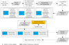 |
Fig. 1 Overall process of RFI-HWT. |
3 Methodology
3.1 Overall process
The overall process of RFI-HWT is depicted in Fig. 1, with the primary steps outlined as follows: (i) preprocessing: read the raw observational data file, extract the time-frequency data matrix, and normalize and segment the data as n normalized data (4096 × 4096); (ii) multi-level 2D WT: apply 2D WT (Li et al. 2021) to the normalized data for three-layer sub-band decomposition, recursively decomposing each layer into low-frequency and high-frequency components as detailed in Fig. 7; (iii) DL integration: employ the DnCNN model (as shown in Fig. 4) (Quan et al. 2021) to process the low-frequency and high-frequency components, enhancing feature selection through a channel-attention mechanism to generate attention weights (Figs. 5 and 6); (iv) RFI elimination: subtract the predicted noise from the original signal components to eliminate interference and combine the cleaned components to form intermediate cleaned data; (v) data reconstruction: utilize an inverse 2D WT to reconstruct the intermediate cleaned data, producing the final cleaned data.
3.2 Data preprocessing
In radio astronomy, data preprocessing is crucial for ensuring the validity and accuracy of analysis results. Observational data are typically stored in the standardized Flexible Image Transport System (FITS) format, which includes extensive metadata and scientific information. A FITS file comprises a header and a data unit. The header contains descriptive information, such as the observation frequency (OBSFREQ), number of observation channels (OBSNCHAN), and observation bandwidth (OBSBW), as well as details about the data unit’s format and content. The data unit stores the actual scientific data, which can be transformed into images, tables, or other forms for further analysis.
The process begins by accessing the Header-Data Units (HDUs) of the FITS file to extract a list of all HDUs. Each HDU contains a dataset and its associated metadata. The second HDU (indexed as 1) includes sub-integration information for the observational data, such as the number of channels, the number of samples, and the sub-integration length. Parsing this HDU yields five-dimensional data: the number of sub-integration blocks, the number of sample points per block, the number of polarization channels, the number of frequency channels, and the data point values. Subsequently, these five-dimensional data are reshaped into the desired two-dimensional time-frequency data format. Data normalization is a crucial step, as it eliminates scale variations arising from different observation conditions. This is achieved through min-max scaling, which standardizes the data’s amplitude or energy to a consistent scale, enhancing algorithm stability and reducing bias during model training. Overall, this systematic approach ensures that the data are well-prepared for subsequent scientific research and discoveries.
3.3 Multi-level 2D WT
The WT is an advanced technique for time-scale signal analysis and serves as a pivotal tool in contemporary signal processing and analysis. Its primary advantage lies in its ability to capture local signal features simultaneously in both the time and frequency domains. By flexibly adjusting the shape, time window, and frequency window of the analysis framework, it facilitates a comprehensive multi-scale analysis of signals, effectively extracting crucial information.
For two-dimensional time-frequency signal matrices, the multi-level 2D WT (Li et al. 2021) is utilized to decompose the signal. This process depends on one two-dimensional scaling function and three 2D wavelet functions, denoted as Eqs. (3), (4), (5), and (6), each of which corresponds to a different decomposition direction. The specific forms of these functions are as follows:
 (3)
(3)
 (4)
(4)
 (5)
(5)
 (6)
(6)
here, h (x) and h (y) are one-dimensional scaling functions along the x and y directions, respectively, while H (x) and H (y) are one-dimensional wavelet functions along the x and y directions, respectively. Using these functions, the signal f (x, y) is transformed into the following form:
 (7)
(7)
where j denotes translation, m denotes x -sampling in the x-dimension with m ∈ [0, 1, 2, …, M – 1], n denotes y-sampling in the y-dimension with n ∈ [0, 1, 2, …, N – 1], the inner product 〈H (0, m, n) h0,m,n (x, y)〉 of H (0, m, n) with h0,m,n (x, y) denotes the approximation parameters of the original data at the scaling level, 〈H1 (j, m, n) hj,m,n (x, y)〉 denotes the wavelet decomposition of the data in the horizontal direction, 〈H2 (j, m, n) hj,m,n (x, y)〉 denotes the wavelet decomposition of the data in the vertical direction, and 〈H3 (j, m, n) hj,m,n (x, y)〉 denotes the wavelet decomposition of the data in the diagonal direction. Therefore, the original two-dimensional time-frequency matrix can be decomposed into three distinct sets of parameters: the approximation parameters at the scaling level, termed as low-frequency features (LL); the decompositions in the horizontal (x) and (y) directions, designated as high-frequency features (HL and LH, respectively); and the decomposition in the diagonal direction, classified as high-frequency features (HH). To validate this approach, a 3328 × 4096 matrix was constructed from down-sampled Parkes telescope data (Fig. 2). Three-layer decomposition (layers 1-3) isolates RFI into distinct spatial-frequency bands (HL/LH/HH), enabling precise RFI localization and suppression, as demonstrated in Fig. 3.
The preprocessed two-dimensional time-frequency data can be recursively decomposed into three layers. Each layer consists of one low-frequency component (LL) and three high-frequency components (HL, LH, HH). The next-level components originate from decomposing the previous level’s LL component. In the inverse wavelet transform and RFI-cleaned low-frequency and high-frequency components are used as inputs. The same wavelet basis employed in the multi-level 2D WT is applied. Beginning from layer 3 down to layer 1, high-frequency details are integrated into the low-frequency approximation using the inverse wavelet filter, layer by layer, until all layers are merged. Ultimately, the inverse wavelet transform reconstructs a clean data matrix, maintaining data integrity and ensuring effective interference mitigation.
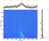 |
Fig. 2 Time-frequency representation of test data. |
3.4 DnCNN network design
The strategy that integrates the DnCNN denoising model with a channel-attention mechanism effectively eliminates RFI from both low-frequency and high-frequency components in each layer, producing interference-free outputs. For each component obtained from the multilayer 2D WT, the DnCNN network structure can be adjusted to accurately identify and remove noise leveraging deep learning techniques. For instance, the HL component of the third layer, with an input size of 525 × 525 × 1, corresponds to the DnCNN network structure shown in Fig. 4. Moreover, the method of the channel-attention mechanism, as illustrated in Fig. 5, involves using the feature maps from either the fifth or 12th layer of the DnCNN model, after convolution, batch normalization, and ReLU activation, as input features. These features are then processed through global average pooling and global max pooling to reduce the spatial dimensions of each channel to 1 × 1 , resulting in two sets of 1 × 1 × 64 feature data. Each set is subsequently passed through two consecutive 1 × 1 convolutional layers with a ReLU activation function in between to introduce nonlinearity. This process generates two sets of channel attention weights, which are then element-wise multiplied with the original input feature maps and summed up, ultimately producing the weighted and optimized feature maps. The mathematical expression for this is shown in Eq. (8):
 (8)
(8)
where P denotes the output image or feature map, S denotes the sigmoid activation function, I1×1 denotes a 1 × 1 convolution, Mc denotes global max pooling across the spatial dimensions, Ac denotes global average pooling across the spatial dimensions, and O denotes the input image or feature map. Fig. 6 illustrates channel-attention weights for the HL component of the first layer, highlighting the attention mechanism’s role in RFI detection. The heat map uses a threshold-based color scheme: red for weights exceeding 0.8 (high relevance) and blue for weights below 0.2 (low relevance). Notably, channels 8, 26, 34, 35, and 55 in Fig. 6 show significantly elevated weights, suggesting their strong relevance to RFI pattern recognition. Furthermore, the DnCNN model is initially trained on labeled samples using a self-training semi-supervised approach (details provided in Section 4.2). This approach aims to minimize dependence on labeled data and enhance the model’s performance in RFI mitigation, especially when labeled data are limited. Ultimately, the RFI-mitigated low-frequency and high-frequency components for the three layers are generated.
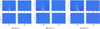 |
Fig. 3 2D WT decomposition for time-frequency signal: layers 1–3 (four subplots per layer displaying multiscale approximation/detail coefficients). |
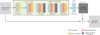 |
Fig. 4 DcCNN network structure for first-layer LH component. The encoding module of DnCNN consists of 17 layers. The first layer begins with 64 3 × 3 convolutional kernels, followed by ReLU activation, and outputs a 525 × 525 × 64 feature map. From the second to the 16th layer, each layer starts with 64 3 × 3 convolutional kernels, followed by batch normalization and then ReLU activation. Specifically, at the fifth and 12th layers, a channel-attention mechanism is introduced after these operations to refine the weighting of the feature maps. Each of these layers outputs a 525 × 525 × 64 feature map. The 17th layer generates a disturbance-estimation map of 525 × 525 × 1 using a single 3 × 3 convolutional kernel. Finally, this disturbance estimation map is subtracted from the original data to obtain clean data with the RFI mitigated, resulting in an output size of 525 × 525 × 1. |
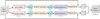 |
Fig. 5 Channel-attention-mechanism network architecture. |
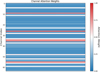 |
Fig. 6 Visualization of channel attention weights for HL component of first layer in RFI detection. |
4 Experiments and results
4.1 Datasets and evaluation metrics
The datasets used in this study are detailed as follows. The training dataset consisted of 400 spectrograms, including 200 from the FRB20201124A data within the fast radio burst (FRB) Key Science Project3 and 200 from the FAST Early Science Project3 and 200 from the FAST Early Science Project4 dataset. We adopted stratified, five-fold cross-validation on the labeled samples (treated as a subset) of these spectrograms, ensuring balanced class representation in each fold. Within each fold, 80% of the samples (i.e., 80 samples) were used for training, and 20% (i.e., 20 samples) for validation. The independent test set comprised 78 spectrograms: 60 (10 per pulsar) from six FAST-observed sources (B1907+02, B1929+10, J1850+0124, J1905+0400, B0320+39, B0523+11) and 18 (3 per pulsar) from six Parkes-observed sources (J0034-0712, J2048-1616, J1136+1551, J0953+0755, J1034-3224, J0529-0715). Critical observational parameters for these pulsars are detailed in Appendix 1. Pulsar names follow the J2000 coordinate system, where “J” is prefixed to the right ascension and declination coordinates (e.g., J1850+0124 indicates right ascension of ~18 h 50 min and declination of ~+01°24′).
The performance of the RFI suppression algorithm is evaluated based on four primary metrics: S/N, Structural Similarity Index Measure (SSIM), RFI Flagging Percentage, and reduced chi-squared  . Among these, the S/N measures the signal strength relative to background noise and serves as a critical metric for assessing the detectability of pulsar signals in the presence of RFI. The SSIM index is employed to quantify the similarity between the clean (label) time-frequency matrix and the RFI-mitigated time-frequency matrix. The format of these matrices is described in Section 3.2. This metric assesses the effectiveness of the RFI mitigation algorithm in preserving the structural information of the pure signal while eliminating interference. The calculation formula is given in Eq. (9):
 (9)
(9)
where x and y represent the clean signal and the RFI mitigated signal, respectively. μx and μy are the means of x and y,  and
and  are the variances of x and y, and σxy is the covariance between x and y. C1 and C2 are small constants used to stabilize the division with weak denominators. Typically, C1 = (K1 L)2 and C2 = (K1 L)2, where L is the dynamic range of the signal values, and K1 and K2 are small constants, typically empirically set to K1 = 0.01 and K2 = 0.03 based on experimental results and practical applications. The RFI flagging percentage represents the proportion of data points flagged as affected by RFI relative to the total number of data points in the dataset, providing a quantitative measure of the extent to which a particular mitigation method identifies data as RFI. The
  is used to assess the significance of periodic signals in the data by comparing observed data with expected data under a specific signal model. It is calculated using following Eq. (10) as follows:
 (10)
(10)
here, Rj denotes the counting rate in the j-th phase bin, μ denotes the mean counting rate, σj denotes the standard deviation in the j-th bin, and n denotes the number of bins. A higher  value indicates a better match between the observed data and the signal model, suggesting more effective RFI mitigation and less signal contamination. In our experiment, RFI flagging is conducted during the “rfifind” processing stage using the Pulsar Exploration and Search Toolkit (PRESTO) software5, which is one of the tools available for this purpose. The S/N and
  values are calculated from the P(Noise) and ;
 values, respectively, provided during the “prepfold” processing stage of PRESTO.
To further validate the robustness of RFI-HWT, we also introduced three widely adopted classification metrics – precision, recall, and F1 score. These metrics, calculated from the confusion matrix generated during RFI detection, collectively assess model performance across diverse operational scenarios. The average values of these metrics, denoted as Precave, Recave, and F1ave, are defined below:
 (11)
(11)
 (12)
(12)
 (13)
(13)
where TPi, FPi, and FNi, respectively, denote true positives (correct RFI detection), false positives (clean signals flagged as RFI), and false negatives (missed RFI) for the i-th sample, and N is the total number of data samples.
Additionally, we calculated the Avg.S/N and the Average Structural Similarity Index Measure (ASSIM) to comprehensively evaluate the algorithm’s RFI mitigation effectiveness. The Avg.S/N represents the mean S/N across all data samples and provides a comprehensive measure of the overall signal quality improvement achieved by the algorithm. It is calculated as follows:
 (14)
(14)
where N is the number of data samples and S/Ni is the S/N of the i-th sample. Similarly, the ASSIM represents the mean SSIM across all data samples and provides a measure of the overall structural similarity between the original and processed data. It is calculated as follows:
 (15)
(15)
where SSIMi denotes the structural similarity index measure of the i-th sample.
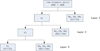 |
Fig. 7 Detailed three-layer wavelet decomposition process. |
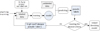 |
Fig. 8 Self-training procedure for semi-supervised learning. |
4.2 Model training
After preprocessing, each sample (a w × 4096 matrix) in the training dataset undergoes three-layer wavelet decomposition as detailed in Section 3.3, producing low-frequency (LL) and high-frequency (HL, LH, HH) components, where w denotes the number of time samples and 4096 represents the number of frequency channels. Each sample is decomposed into one approximation coefficient layer and three detail coefficient layers, which are represented as [LL3, [HL1, LH1, HH1], [HL2, LH2, HH2], [HL3, LH3, HH3]]. Subscripts indicate the decomposition levels; for example, LH1 is the vertical component of the first layer. Empirically, LL3, HL1, HL2, and HL3 are identified as the dominant interference sources, whereas other high-frequency components (lower power density) are omitted during training. Fig. 7 illustrates the detailed decomposition process and data sizes of the components. For oversized time-frequency matrices (w > 4096), the data are segmented into 4096 × 4096 sub-matrices. Each sub-matrix undergoes independent RFI mitigation and is subsequently reassembled into the original w × 4096 matrix.
As detailed in Section 4.1, the training dataset comprises 400 spectrograms: 180 labeled and 220 unlabeled. The labeled samples are paired with corresponding “clean” counterparts, which refer to denoised spectrograms reconstructed from inpainted data. The training procedure, illustrated in Fig. 8, is conducted as follows. The model is initially trained on labeled samples for supervised learning. Specifically, we used stratified five-fold cross-validation on the 180 labeled samples, with each fold containing 144 training samples and 36 validation samples to ensure balanced class representation. Subsequently, the model undergoes semi-supervised five-fold cross-validation on the entire dataset, including both labeled and unlabeled samples. In each fold, the model predicts the unlabeled samples, converts these predictions into pseudo-labels via inverse wavelet transforms, and incrementally incorporates high-confidence pseudo-labeled samples into the training set. This cycle of training, predicting, generating pseudo-labels, and retraining continues until the model demonstrates satisfactory performance across all folds.
Table 1 lists the key training parameters for each component. The learning rate (LR) and optimizer are set uniformly across all components. Typically, the LR is selected through empirical methods, often starting with a standard value such as 0.001 and then adjusted based on the model’s convergence behavior. The optimizer, chosen for its efficiency and adaptability, is typically set to Adam due to its proven effectiveness in deep learning applications. The Batch_Size is determined based on resource constraints (including dataset size and hardware limitations) as well as model complexity and training objectives. To prevent GPU and RAM bottlenecks under resource constraints, the Batch_Size must be restricted to a small range (1–4). The loss function, mean squared error (MSE), is computed by reconstructing the denoised wavelet coefficients into a spectrogram via inverse wavelet transform and then averaging the squared differences between this reconstructed spectrogram and the clean ground-truth spectrogram. This ensures the loss is evaluated in the original data domain for effective training.
Different model-training parameters.
4.3 Parallelization
As a combination of 2D WT and DnCNN methods, RFI-HWT exhibits a more complex serial process than the standalone 2D WT algorithm. To efficiently manage this complexity, we utilized Compute Unified Device Architecture (CUDA)6, a platform for heterogeneous computing that leverages both CPU and GPU resources to harness the parallel processing capabilities of modern GPUs. In CUDA, the thread hierarchy is structured into blocks of threads and grids of blocks, with the efficient arrangement of these threads being vital, given the independence of the data being processed. During the multilevel 2D WT described in Section 3.3, raw observational data was decomposed into various components across three layers, which were then aggregated into a single batch. This batch was processed concurrently within the DnCNN model to eliminate RFI, leveraging CUDA’s parallel processing power. Moreover, each layer of the RFI elimination process can handle multiple samples simultaneously, similarly to data parallelism in DL, fully exploiting GPU parallelism.
Briefly, incorporating batch processing into both training and inference phases significantly speeds up DnCNN model training and convergence. By combining CUDA parallelization with batch processing in the RFI-HWT algorithm, execution time can be significantly reduced compared to sequential processing, leading to substantial performance improvements. This is crucial for efficiently handling large-scale radio astronomical datasets and ensuring scalable, effective RFI mitigation.
Parameters used in Preprold.
4.4 Results analysis and discussion
Our algorithm was tested on a Linux cluster with seven physical nodes, each equipped with an Intel 6230 Xeon CPU at 2.1 GHz, totaling 480 cores. The cluster also featured four Nvidia GeForce RTX 2080 Ti GPUs, 5.3TB of RAM, and 3.6PB of disk space. The system is running Linux 3.10.0-862. el7.x86_64, PRESTO, Anaconda3-4.2.0, Python 3.8, CUDA 11.0, and PyTorch 1.7.1+cu110. To evaluate the RFI-HWT algorithm’s mitigation efficacy, we compared it with the “rfifind” in the PRESTO pipeline, the original 2D WT method (Li et al. 2021), and two representative DL-based approaches: RFI-Net (Yang et al. 2020) and the recent RFDL framework (van Zyl & Grobler 2024). All these methods were executed under identical hardware and software conditions. PRESTO is widely used for pulsar detection and astrophysical signal processing. Its workflow effectively handles RFI using the rfifind program, which generates a “mask” file that is crucial for subsequent folding processing to produce a “prepfold” file. For accurate performance assessment, the RFI-HWT, 2D WT, RFI-Net, and RFDL methods were integrated into the PRESTO pipeline, replacing rfifind during the comparative analysis. Table 2 presents the parameter settings used in the “prepfold” processing, and the information related to these parameters can be queried in the psrcat7 database.
Tables 3 and 4 present a performance comparison of five methods on the FAST dataset. Table 3 shows that RFI-HWT consistently outperforms the other four methods in Avg.S/N and ASSIM across all test samples. Table 4 further demonstrates that RFI-HWT generally achieves higher Precave, Recave, and F1ave scores than the other methods on the FAST dataset. Tables 5 and 6 show the overall performance comparison of these methods on the Parkes dataset. Notably, the RFI-HWT model trained on FAST data demonstrates good generalization capability when applied to data from the Parkes telescope. As shown in Tables 5 and 6, RFI-HWT consistently achieves the highest Avg.S/N, ASSIM, Precave, Recave, and F1ave values among all compared methods, including RFI-Net and RFDL, on the Parkes dataset.
Across both the FAST and Parkes datasets, RFI-HWT achieves significant superiority in RFI suppression capabilities over other methods. Specifically, compared to rfifind, it improves Avg.S/N by approximately 15% and ASSIM by about 14%. Relative to the 2D WT method, it enhances Avg.S/N by roughly 11% and ASSIM by around 12%, with these improvements averaged across all test samples. Additionally, RFI-HWT exhibits an average improvement of approximately 3.26% in Avg.S/N and 4.46% in ASSIM compared to RFI-Net. Compared with RFDL, it shows a 2.12% enhancement in Avg.S/N and a 2.71% improvement in ASSIM.
Specifically, samples were arbitrarily selected for further in-depth analysis. As depicted in Fig. 9a, a comprehensive comparison of five methods (i.e., rfifind, 2D WT, RFI-NET, RFDL, and the proposed RFI-HWT) on a B1929+10 sample reveals that RFI-HWT performs better across nearly all evaluation metrics except computational efficiency. Obviously, it exhibits the highest RFI flagging accuracy and offers significant  while maintaining notable S/N enhancement and SSIM performance, indicating its superior ability in preserving astrophysical signal morphology. Moreover, the CUDA-parallelized implementation of RFI-HWT exhibits a lower execution time compared to 2D WT, although it is slightly higher than that of rfifind, RFI-Net, and RFDL. Notably, the CUDA-parallelized RFI-HWT implementation has a shorter execution time than 2D WT, but it is slightly longer than those of rfifind, RFI-Net, and RFDL. It should be noted that the time consumption for RFI-HWT here only refers to the inference phase, including signal matrix decomposition, component-wise RFI mitigation, and signal reconstruction, while excluding model training overhead. This evaluation approach aligns with the protocols used for RFI-Net and RFDL. This suggests that its parallel mode using CUDA can improve execution efficiency while maintaining accurate RFI mitigation. Fig. 9b shows a comprehensive comparison of the five methods on a PKS J0953+0755 sample, with results similar to those in Fig. 9a.
Figures 10 and 11 present the integrated profiles of B1929+10 and PKS J0953+0755 obtained using the five methods, respectively. It can be observed that, compared to rfifind, 2D WT, RFI-Net, and RFDL, our method effectively eliminates outliers and yields smoother integrated profiles. Figs. 12 and 13 present comparisons of the time-frequency diagrams for the B1929+10 and PKS J0953+0755 samples, respectively. Fig. 12a highlights the transient interference observed at specific locations within the raw data. Fig. 12b shows the ideal time-frequency signal intensity after all RFI has been completely removed. Figs 12c–12f illustrate that rfifind (S/N=320.4 σ / SSIM=86.1%), the 2D WT (S/N=323.8 σ / SSIM=89.4%), RFI-Net (S/N=328.9 σ / SSIM=93.2%), and RFDL (S/N=322.6 σ / SSIM=88.3%) can partially mitigate this interference but fail to completely eliminate it. In contrast, as illustrated in Fig. 12g, the RFI-HWT algorithm achieves S/N=331.6 σ and SSIM=95.2%, indicating near-total suppression of RFI while preserving the original pulsar signal characteristics. Notably, within the spectral region bounded by the two red markers, our methodology achieves marked interference attenuation, closely approaching the intensity level depicted in Fig. 12b. Furthermore, Figs. 12h–12l, respectively, show the difference spectrograms for RFIfind, 2D WT, RFI-Net, RFDL, and RFI-HWT algorithms. These visualizations demonstrate algorithmic performance through spectral differences before and after processing. Warm-colored positive regions indicate successful interference removal, while cool-colored negative regions may suggest poor processing or the introduction of new interference. Notably, Fig. 12l displays concentrated positive regions, demonstrating effective local interference removal. Despite still-existing negative regions, its localized performance indicates comparatively superior overall RFI suppression, and its localized performance indicates comparatively superior overall RFI suppression. Conversely, other figures exhibit either limited positive regions or widespread negative dominance, indicating less satisfactory suppression performance.
Figure 13a presents a variety of interference types found in the raw data, including impulsive interference, narrowband interference, and broadband interference, while Fig. 13b shows the ideal interference-free signal. As demonstrated in Figs. 13c–13g, all five methods effectively mitigate these interferences, with red-framed regions highlighting critical RFI areas. Notably, RFI-HWT achieves superior performance (S/N=44.6 σ / SSIM=97.0%) compared to rfifind (S/N=38.1 σ / SSIM=85.3%), 2D WT (S/N=39.3 σ / SSIM=87.4%), RFI-Net (S/N=41.6 σ / SSIM=91.4%), and RFDL (S/N=44.1 σ / SSIM=96.3%), demonstrating better interference suppression and S/N improvement. However, our approach still lags behind the ideal baseline in Fig. 13b regarding complete RFI detection. Difference spectrograms in Figs. 13h–13l further reveal that both RFI-HWT (Fig. 13l) and RFDL (Fig. 13k) exhibit superior RFI removal with similar positive region patterns. RFI-HWT shows denser red stripes, indicating stronger suppression capability than RFDL at specific time-frequency coordinates.
The results on the FAST and Parkes datasets reveal that RFI-HWT significantly outperforms both traditional algorithms (rfifind and 2D WT) and recent deep-learning-based approaches (RFI-Net and RFDL) across key metrics: Avg.S/N, ASSIM,  , RFI Flagging Percentage, Precave, Recave, and F1ave . Specifically, RFI-HWT achieves average improvements of 3.26% in Avg.S/N and 4.46% in ASSIM over RFI-Net, and 2.12% in Avg.S/N and 2.71% in ASSIM over RFDL on both datasets. In summary, these findings demonstrate the effectiveness of RFI-HWT in mitigating various RFI types and balancing the evaluated metrics. Consequently, we conclude that the proposed hybrid approach, which integrates the multi-scale and multidirectional decomposition of 2D WT with the robust feature extraction and noise suppression capabilities of DnCNN and is augmented by a self-training semi-supervised learning strategy, provides a powerful solution for enhancing the quality of radio astronomical observations. Furthermore, with adequate model training, our proposed method can identify and mitigate diverse RFI sources within complex astronomical signals. However, despite the significant contributions of RFI-HWT to mitigating RFI, it is crucial to consider its computational efficiency and practicality. Although the running time decreases with the addition of parallel nodes, its overall computational requirements still need further improvement, particularly when processing large-scale datasets. This may pose challenges for real-time processing and deployment in resource-constrained environments. While RFI-HWT generalizes well across known datasets, its adaptability to novel types of RFI requires further validation. Additionally, the presence of residual noise in high-frequency components suggests there is room for further optimization to enhance feature extraction precision. These limitations can be addressed through ongoing research and development.
Comparison results on FAST dataset in Avg.S/N(σ) /ASSIM(%).
Comparison results on FAST dataset in Precave (%) / Recave(%) / F1ave(%).
Comparison results on Parkes dataset in Avg.S/N(σ) /ASSIM(%).
Comparison results on Parkes dataset in Precave (%) / Recave(%) / F1ave(%).
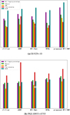 |
Fig. 9 Comprehensive comparison of five methods applied to data samples containing B1929+10 and PKS J0953+0755. |
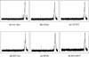 |
Fig. 10 Integration contour plots for B1929+10 using five methods. |
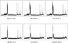 |
Fig. 11 Integration contour plots for PKS J0953+0755 using five methods. |
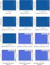 |
Fig. 12 Comparison of time-frequency plots for five methods on a B1929+10 sample. |
5 Conclusions
In this paper, we present RFI-HWT, a hybrid deep learning algorithm aimed at tackling the challenges of RFI mitigation in high-sensitivity radio astronomy. By integrating the multilevel 2D WT with a denoising convolutional neural network (DnCNN), our algorithm effectively leverages multi-scale and multidirectional signal decomposition to identify and eliminate RFI, thereby improving the quality of observational data. The adoption of a self-training, semi-supervised learning approach enhances the model’s generalization capability, allowing it to handle both labeled and unlabeled datasets. Through preliminary experiments with real observational data from the FAST and Parkes telescopes, the feasibility of RFI-HWT has been demonstrated. Furthermore, the parallelized implementation of RFI-HWT ensures efficient processing of large-scale datasets.
Future work will focus on optimizing the model’s architecture to reduce computational complexity while preserving its performance. This can be accomplished by exploring more efficient network designs and leveraging parallel computing techniques. Additionally, strategies for continuous learning and transfer learning will be explored to enable the model to rapidly adapt to new types of RFI and varying environments. This will ensure that the model maintains high performance consistently over time and across different astronomical signals. The program codes of RFI-HWT were uploaded online8.
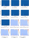 |
Fig. 13 Comparison of time-frequency plots for five methods on a PKS J0953+0755 sample. |
Acknowledgements
This research is partially supported by the National Key R&D Program of China (No. 2022YFE0133700), the National Science Foundation of China (NSFC, grant Nos. 12273008, 11963003, 12273007, and 62062025), the National SKA Program of China (No. 2020SKA0110300), the Guizhou Province Science and Technology Support Program (General Project, No. Qianhe Support [2023] General 333), the Science and Technology Foundation of Guizhou Province (Key Program, No. [2019]1432), the Guizhou Provincial Science and Technology Projects (Nos. ZK[2022]143 and ZK[2022]304), and the Cultivation Project of Guizhou University (No. [2020]76). This work made use of the data from FAST (Five-hundred meter Aperture Spherical radio Telescope). FAST is a Chinese national mega-science facility, operated by National Astronomical Observatories, Chinese Academy of Sciences.
Additionally, we acknowledge the use of data from the Parkes telescope, which significantly enhanced the scope of this study.
Appendix A Critical observational parameters for the 12 Pulsars in the test set
| names/Parameters | telescope | P(s) | DM (pc/cm3) | S1400 (mJy) | PEpoch (MJD) | S400 (mJy) | RM (rad m–2) | W10 (ms) | F0 (Hz) |
|---|---|---|---|---|---|---|---|---|---|
| B1907+02 | FAST | 0.989831207210 | 171.7 | 0.63 | 49695.0 | 21.0 | 266.5 | 12.1 | 1.0102685320583 |
| GB1929+10 | FAST | 0.2265187466568 | 3.18 | 29 | 57600 | 303 | –6.950 | 14.7 | 4.4146421450799 |
| J1850+0124 | FAST | 0.003559763768043 | 118.88 | 0.188 | 5583 | * | –68.9 | * | 280.9175173300 |
| J1905+0400 | FAST | 0.0037844047882356 | 25.6 | 0.050 | 53700 | * | 36.9 | 113.3 | 264.24234614348 |
| B0320+39 | FAST | 3.032071956385 | 26.1898 | 0.9 | 49290.0 | 34 | 60.00 | 74.7 | 0.3298074763345 |
| B0523+11 | FAST | 0.35443759451370 | 79.42 | 1.94 | 48262.0 | 19.5 | 4.4 | 22.3 | 2.8213705328215 |
| J0034-0721 | Parkes | 0.9429509945598 | 10.922 | 11 | 46635.0 | 52 | 8.3 | 120 | 1.060499976 |
| J2048-1616 | Parkes | 1.961572303613 | 11.456 | 22 | 46423.0 | 116 | –10.520 | 84 | 0.5097919243998 |
| J1136+1551 | Parkes | 1.187913065936 | 4.8407 | 20 | 46407.0 | 257 | 2.56 | 34 | 0.8418094604365 |
| J0953+0755 | Parkes | 0.2530651649482 | 2.96927 | 100 | 46375.0 | 400 | –0.45 | 21 | 3.951547269235 |
| J1034-3224 | Parkes | 1.150590428417 | 50.75 | 8 | 50705.0 | 41 | –46.0 | 306 | 0.869118853459 |
| J0529-0715 | Parkes | 0.689223601359 | 87.3 | 0.125 | 58372.0 | * | –46 | 26.3 | 1.450907946316 |
References
- Callingham, J., Dijkema, T., de Gasperin, F., et al. 2019, A&A, 622, A1 [NASA ADS] [CrossRef] [EDP Sciences] [Google Scholar]
- Fu, Z., Zhang, H., Zhao, J., Li, N., & Zheng, F. 2023, Remote Sens., 15, 846 [Google Scholar]
- Li, L., Gaiser, P. W., Bettenhausen, M. H., & Johnston, W. 2006, IEEE Trans. Geosci. Remote Sens., 44, 530 [Google Scholar]
- Li, W., Xu, H., Ma, Z., et al. 2019, ApJ, 879, 104 [Google Scholar]
- Li, H.-S., Fan, P., Peng, H., Song, S., & Long, G.-L. 2021, IEEE Trans. Cybern., 52, 8467 [Google Scholar]
- Mesarcik, M., Boonstra, A.-J., Ranguelova, E., & van Nieuwpoort, R. V. 2022, MNRAS, 516, 5367 [NASA ADS] [CrossRef] [Google Scholar]
- Mitchell, D., Robertson, J., & Sault, R. 2005, ApJ, 130, 2424 [Google Scholar]
- Offringa, A., De Bruyn, A., Biehl, M., et al. 2010, MNRAS, 405, 155 [NASA ADS] [Google Scholar]
- Pen, U.-L., Chang, T.-C., Hirata, C. M., et al. 2009, MNRAS, 399, 181 [Google Scholar]
- Quan, Y., Chen, Y., Shao, Y., et al. 2021, Pattern Recognit., 111, 107639 [Google Scholar]
- Rafiei-Ravandi, M., & Smith, K. M. 2023, ApJS, 265, 62 [Google Scholar]
- Sardarabadi, A. M., van der Veen, A.-J., & Boonstra, A.-J. 2015, IEEE Trans. Signal Process., 64, 432 [Google Scholar]
- Shan, H., Yuan, J., Wang, N., & Wang, Z. 2022, ApJ, 935, 117 [Google Scholar]
- Smits, R., Lorimer, D., Kramer, M., et al. 2009, A&A, 505, 919 [NASA ADS] [CrossRef] [EDP Sciences] [Google Scholar]
- Song, Y., Liu, Z., Wang, N., Li, J., & Yuen, R. 2021, ApJ, 922, 94 [Google Scholar]
- Sun, H., Deng, H., Wang, F., et al. 2022, MNRAS, 512, 2025 [NASA ADS] [CrossRef] [Google Scholar]
- Tian-qi, L., Ya-jun, W., Ren-jie, Z., & Zhi-jun, X. 2021, Chin. Astron. Astrophys., 45, 587 [Google Scholar]
- Vafaei Sadr, A., Bassett, B. A., Oozeer, N., Fantaye, Y., & Finlay, C. 2020, MNRAS, 499, 379 [NASA ADS] [CrossRef] [Google Scholar]
- van Zyl, D. J., & Grobler, T. L. 2024, MNRAS, 530, 1907 [Google Scholar]
- Yan, R.-Q., Dai, C., Liu, W., et al. 2021, Res. Astron. Astrophys., 21, 119 [Google Scholar]
- Yang, Z., Yu, C., Xiao, J., & Zhang, B. 2020, MNRAS, 492, 1421 [NASA ADS] [CrossRef] [Google Scholar]
- Zhang, Y.-J., Li, Y.-Z., Cheng, J., & Yan, Y.-H. 2021, Res. Astron. Astrophys., 21, 299 [Google Scholar]
All Tables
All Figures
|
Fig. 1 Overall process of RFI-HWT. |
| In the text | |
|
Fig. 2 Time-frequency representation of test data. |
| In the text | |
|
Fig. 3 2D WT decomposition for time-frequency signal: layers 1–3 (four subplots per layer displaying multiscale approximation/detail coefficients). |
| In the text | |
|
Fig. 4 DcCNN network structure for first-layer LH component. The encoding module of DnCNN consists of 17 layers. The first layer begins with 64 3 × 3 convolutional kernels, followed by ReLU activation, and outputs a 525 × 525 × 64 feature map. From the second to the 16th layer, each layer starts with 64 3 × 3 convolutional kernels, followed by batch normalization and then ReLU activation. Specifically, at the fifth and 12th layers, a channel-attention mechanism is introduced after these operations to refine the weighting of the feature maps. Each of these layers outputs a 525 × 525 × 64 feature map. The 17th layer generates a disturbance-estimation map of 525 × 525 × 1 using a single 3 × 3 convolutional kernel. Finally, this disturbance estimation map is subtracted from the original data to obtain clean data with the RFI mitigated, resulting in an output size of 525 × 525 × 1. |
| In the text | |
|
Fig. 5 Channel-attention-mechanism network architecture. |
| In the text | |
|
Fig. 6 Visualization of channel attention weights for HL component of first layer in RFI detection. |
| In the text | |
|
Fig. 7 Detailed three-layer wavelet decomposition process. |
| In the text | |
|
Fig. 8 Self-training procedure for semi-supervised learning. |
| In the text | |
|
Fig. 9 Comprehensive comparison of five methods applied to data samples containing B1929+10 and PKS J0953+0755. |
| In the text | |
|
Fig. 10 Integration contour plots for B1929+10 using five methods. |
| In the text | |
|
Fig. 11 Integration contour plots for PKS J0953+0755 using five methods. |
| In the text | |
|
Fig. 12 Comparison of time-frequency plots for five methods on a B1929+10 sample. |
| In the text | |
|
Fig. 13 Comparison of time-frequency plots for five methods on a PKS J0953+0755 sample. |
| In the text | |
Current usage metrics show cumulative count of Article Views (full-text article views including HTML views, PDF and ePub downloads, according to the available data) and Abstracts Views on Vision4Press platform.
Data correspond to usage on the plateform after 2015. The current usage metrics is available 48-96 hours after online publication and is updated daily on week days.
Initial download of the metrics may take a while.