| Issue |
A&A
Volume 701, September 2025
|
|
|---|---|---|
| Article Number | A59 | |
| Number of page(s) | 13 | |
| Section | Interstellar and circumstellar matter | |
| DOI | https://doi.org/10.1051/0004-6361/202554479 | |
| Published online | 03 September 2025 | |
Isentropic instability and dynamic substructures in the Orion Bar photodissociation region: Analytical and numerical insights
1
Department of Theoretical Physics, Lebedev Physical Institute,
Samara,
Russia
2
Department of Physics, Samara National Research University,
Samara,
Russia
★ Corresponding authors.
Received:
11
March
2025
Accepted:
15
July
2025
Abstract
Context. The Orion Bar photodissociation region (PDR), which is shaped by far-ultraviolet (FUV) radiation, displays filamentary substructures and non-thermal gas motions across its ionized, atomic, and molecular zones, as observed by ALMA, JWST, and other telescopes, suggesting dynamic processes beyond static equilibrium.
Aims. Our goal is to test isentropic instability as a mechanism for these features, focusing on the atomic zone’s shockwave structures and their alignment with observational data.
Methods. We adapted gasdynamic equations to derive analytical solutions for shockwave pulse properties and complemented them with numerical simulations to track their evolution under varying initial conditions while incorporating a heat-loss function reflecting Orion Bar conditions.
Results. Our analytical and numerical results yield pulse widths (∼0.001 pc) and periods (∼0.02 pc) that closely match the observed substructure sizes (0.002–0.004 pc) and separations (0.01 pc), while the velocity amplitudes (0.72 cS) agree with non-thermal estimates. The leading pulse amplitude reaches a stationary value within 5000–40 000 years, which is well within the estimated ∼105−year lifetime of the Orion Bar PDR.
Conclusions. This study demonstrates that isentropic instability can reproduce the Orion Bar’s dynamic features, bridging theoretical predictions and high-resolution observations from ALMA and JWST.
Key words: instabilities / shock waves / ISM: clouds / photon-dominated region (PDR) / ISM: individual objects: Orion Bar
© The Authors 2025
 Open Access article, published by EDP Sciences, under the terms of the Creative Commons Attribution License (https://creativecommons.org/licenses/by/4.0), which permits unrestricted use, distribution, and reproduction in any medium, provided the original work is properly cited.
This article is published in open access under the Subscribe to Open model. This email address is being protected from spambots. You need JavaScript enabled to view it. to support open access publication.
1 Introduction
The thermal instability of optically thin plasma, which undergoes heating and radiative cooling, has attracted considerable attention since the seminal works of Parker (1953) and Field (1965). In astrophysics, the primary motivation for studying thermal instabilities lies in explaining the formation of dense localized structures with masses insufficient for gravitational compression. According to Field (1965), thermal instabilities can be classified into three types: isochoric, isobaric, and isentropic instabilities. Of these, only the last two can lead to stationary or oscillating condensations within an initially homogeneous medium.
The isochoric instability generates exponential temperature growth that remains spatially uniform throughout the unstable region, avoiding distinct structural formation. However, according to Field (1965), pressure variations associated with temperature changes under isochoric conditions generally induce fluid motions that disrupt the constant density required for the instability to be sustained.
The most well-known instability in astrophysics is the isobaric instability, which results in the stratification of the medium into hot rarefied gas and dense cold clumps at constant pressure. Consequently, it is often referred to as the condensation instability. This type of instability is relevant to a wide range of astrophysical phenomena, including condensations in planetary nebulae (e.g., Zanstra 1955), the two-phase model (Field 1965; Goldsmith et al. 1969), and multiphase models of interstellar clouds (e.g., Jennings & Li 2021). Isobaric instability is also associated with high-density clumps and filaments in quiescent diffuse star-forming clouds (Wareing et al. 2016), solar prominences (e.g., Smith & Priest 1977; Priest & Smith 1979; Xia & Keppens 2016), and coronal rain (e.g., Claes & Keppens 2019). Additionally, it has been explored in the context of molecular loops in the Galactic central region (Peng & Matsumoto 2017), the origin of cold gas in galactic clusters and haloes (Ji et al. 2018), and the vertical thermal collapse of thin disks accreting onto stellar-mass black holes (Fragile et al. 2018), among others.
In this paper, we focus on the nonlinear manifestations of another type of thermal instability: isentropic (acoustic) instability. Unlike isobaric instability, which leads to the formation of stationary dense condensations at constant pressure, isentropic instability results in the amplification of acoustic waves. Consequently, denser regions become hotter and exhibit a higher pressure compared to the rarefied surroundings. These regions propagate through space at the speed of sound in the linear approximation. Moreover, in contrast to the isobaric case, density perturbations in the stationary state are accompanied by gas motion.
It has been demonstrated that the conditions for isentropic (acoustic) instability are met in various astrophysical media. For instance, Oppenheimer (1977), Krasnobaev & Tarev (1987), and Krasnobaev (2000) have shown that this instability can occur in interstellar molecular clouds near hot stars. These clouds, composed primarily of molecular hydrogen with minor admixtures of grains and CO molecules, are heated by collisions with hot grains and cooled by radiation in the rotational lines of CO. Similarly, Flannery & Press (1979) and Dudorov et al. (2019) investigated acoustic instability in diffuse cold interstellar clouds using a model of the interstellar medium in which heating and ionization result from cosmic ray interactions with atoms, molecules, and grains, while cooling occurs due to electron collisional excitation of C+. Isentropic instability has also been studied in other media, including the Earth’s ionosphere (Suleimenov et al. 2006), solar corona plasma (Ibanez & Sanchez 1992; Nakariakov et al. 2000; Molevich et al. 2016; Zavershinskii et al. 2019), and even near black hole horizons (Parikh & Wilczek 1998).
The isentropic instability has been most extensively studied in the atomic zones of photodissociation regions (PDRs; Molevich et al. 2011; Krasnobaev et al. 2016; Krasnobaev & Tagirova 2017, 2019; Zavershinskii et al. 2020; Molevich & Riashchikov 2021; Riashchikov et al. 2022). Analytical and numerical studies have shown that, at the nonlinear stage, isentropic instability leads to the formation of self-sustaining, quasi-periodic structures characterized by increased density, temperature, pressure, and velocity (multiple shock waves). A characteristic profile of such structures is illustrated in Figure 1. As highlighted in Krasnobaev & Tagirova (2017), these multiple shock waves can manifest as filamentary or reticulate structures, not only in the HI zone but also in ionized gas due to the penetration of perturbations into the HII region. Similar structures have also been observed penetrating the molecular zone of PDRs.
The structures formed by isobaric and isentropic instabilities exhibit notable differences. Isobaric instability primarily results in the stratification of the medium into quasi-static, cold dense regions (clouds) and a hot rarefied medium. In contrast, isentropic instability is characterized by the emergence of dynamic quasi-periodic multi-front structures that propagate at supersonic speeds. These structures, due to their shockwave nature, feature sharp perturbation fronts where density, pressure, temperature, and velocity undergo rapid changes. Estimates for PDRs (Krasnobaev & Tagirova 2017) suggest that the thickness of these shock fronts is on the order of an astronomical unit or less. Behind the sharp fronts, the medium’s parameters change more gradually. It is useful to define a characteristic scale, L1, as the distance over which the magnitude behind the wavefront decreases by a factor of e. The characteristic periodicity of these structures, denoted as L2, is also illustrated in Figure 1.
Recent observations have provided substantial evidence of the existence of similar shockwave structures in PDRs. The Orion Bar PDR, being the closest PDR to the Solar System (at a distance of ~414 ± 7 pc), has been the subject of numerous studies. Indirect evidence of small-scale regions of rapidly increasing gas velocity comes from the analysis of non-thermal line widths in the Orion Nebula (Ferland et al. 2012). Ferland investigated the NI pumping zone and demonstrated that a non-thermal broadening mechanism must operate at scales of a few astronomical units, likely driven by small-scale thermal instabilities of neutral gas in the temperature range ~1000-3000 K.
Advances in the resolution of ground-based and space telescopes have enabled direct and detailed studies of smallscale structures. The Atacama Large Millimeter Array (ALMA) obtained the first ~1″ resolution images of CO and HCO+ emission in the Orion Bar (Goicoechea et al. 2016), revealing rich substructures such as filaments, globulettes, and ripples with increased density and pressure moving into the molecular region. These substructures, observed near the dissociation front (DF) and in the atomic region, have characteristic sizes of ~2″ (~4.0 × 10⁻³ pc) and are spaced at roughly periodic distances of about 5″ (≈0.01 pc). These differ from the larger (~5″-10″) condensations previously observed deeper within the molecular cloud (Owl et al. 2000; Lis & Schilke 2003). The findings of Goicoechea et al. (2016) were further corroborated and expanded by Joblin et al. (2018) and Habart et al. (2023).
Joblin et al. (2018) analyzed high-J CO emission lines (where J is the rotational quantum number) in two PDR prototypes (Orion Bar and NGC7023 NW) using data from the Herschel Space Observatory. They concluded that high-J CO line emission originates from small structures with typical thicknesses of ~10−3 pc and at high thermal pressures in the Orion Bar.
Habart et al. (2023) confirmed that the edge of the Orion Bar is composed of small, dense substructures at high thermal pressure embedded in a more diffuse medium. Observations with the Keck/Near Infrared Camera 2 (NIRC2) spatially resolved numerous irradiated substructures, including ridges, filaments, globules, and proplyds. Peaks of H2 emission were detected starting from ~10″ from the ionization front (IF) and extending up to ~20″ or even 25″-30″ in some regions. These peaks exhibit sharp fronts toward the IF and are spaced by a few arcseconds (0.005-0.01 pc or ~1000-2000 au). Bright substructures such as ridges and filaments with widths of 1″-2″ (0.0020.004 pc or 400–800 au) run parallel to the DF. Additionally, a series of bright substructures in H2 emission were observed toward the molecular region.
The James Webb Space Telescope (JWST) has provided the most detailed and sharpest images of the Orion Nebula, including high-resolution infrared spectral imaging of the Orion Bar PDR with an angular resolution of 0.075″ up to 0.173″ (1.5-3.46 × 10⁻⁴ pc at 414 pc) (Habart et al. 2024; Peeters et al. 2024). These images reveal that the molecular cloud borders are highly structured at small scales of 0.1″-1″ (0.0002-0.002 pc or 40–400 au). Numerous small-scale structures, such as ridges, waves, globules, and proplyds, are evident. The spatial distribution of the aromatic infrared bands (AIBs) indicates that the PDR edge is very steep (on scales of 1″ or 0.002 pc), with a sharp density rise in the neutral zone followed by an extensive warm atomic layer with number density nH = (0.5– 1.0) × 105 cm−3 up to the DF, where multiple ridges are observed. The transition from the atomic to the molecular PDR is highly structured, displaying three terraced-like DFs overlaid with numerous smaller-scale structures (of a few 0.1″).
Similar substructures have been observed in other PDRs, where resolution permits. For example, infrared images of the Horsehead Nebula captured by JWST (Abergel et al. 2024) reveal filamentary structures in the 1–0 S(1) line of H2 at the illuminated edge of the PDR on scales as small as 1.5″ (2.0 × 10⁻³ pc), with numerous sharp substructures on even smaller scales. Zemlyanukha et al. (2022) reported the first evidence of a clumpy HI environment in the S187 PDR, located 1.4 ± 0.3 kpc from the Solar System.
In the Carina Nebula, dynamic high-pressure structures moving at supersonic velocities were detected using observations from the Herschel Space Observatory (Wu et al. 2018), ALMA (Hartigan et al. 2022; Downes et al. 2023), and the Gemini telescope (Hartigan et al. 2020). ALMA’s angular resolution (~1″) at a distance of 2.3 kpc resolved clumps in the Carina’s Western Wall with sizes exceeding 0.01 pc. In Hartigan et al. (2022), it was found that the internal turbulent velocity dispersion within individual clumps of this spatial scale is comparable to the sound speed of the gas and tends to be higher in more massive clumps. The velocity between clumps was typically three to five times the sound velocity. Using high-resolution ALMA observations, Downes et al. (2023) presented a variety of investigations of the turbulent dynamics of PDR boundary in the Carina’s Western Wall and length-scales. It was obtained that shock waves dominate the turbulence and that length scales in the range 0.02-0.03 pc are important in the dynamics of the Western Wall. The Gemini telescope achieved subarcsecond resolution (~0.06″-0.11″), revealing spaced ridges, filaments, and waves in the Western Wall molecular cloud with spatial scales between 0.001-0.01 pc (or 200-2000 au) (Hartigan et al. 2020).
Given the wealth of observational data, the origin of these substructures remains a key question. In Peeters et al. (2024), following the hypothesis proposed by Goicoechea et al. (2016), small-scale substructures are attributed to preexisting, turbu-lently driven density variations, such as those developing during the passage of shock waves due to isentropic thermal instability (Molevich et al. 2011; Krasnobaev et al. 2016; Krasnobaev & Tagirova 2017; Riashchikov et al. 2022).
In this paper, we further develop a hypothesis linking the observed structures in PDRs to isentropic instability as a driver for their emergence. We aim to identify the key parameters that govern the formation and evolution of these structures. Specifically, we seek to estimate the characteristic spatial scales of these structures, such as the width of individual shockwave pulses (L1) and the distance between neighboring pulses (L2), as well as their amplitude (A) and the time required for their formation in the atomic zone of the Orion Bar PDR. Understanding these parameters will provide insights into the physical processes driving the observed substructures and help bridge the gap between theoretical models and observational data.
Our paper is organized as follows. First, in Section 2, we describe the basic system of equations and the heat-loss function, which is acceptable for the Orion Bar PDR atomic zone, and provide numerical values of the main parameters of this function. In Section 3, we present two approaches to analyze optically thin plasma, which undergoes some heating and radiative cooling. Sections 3.1 and 3.2 conclude with a clarification of analytical and numerical approaches. Section 4 is divided into four parts. First, in Section 4.1, we present an estimation of the pulse amplitude, A, and the characteristic scale, L1, obtained with the analytical method. In Section 4.2, we examine the early stage of gasdynamic disturbance evolution. In Section 4.3, we estimate the distance between a pair of peaks, L2, and discuss the autowave nature of investigated pulses. In Section 4.4, we examine the time required for the leading pulse to attain the stationary amplitude predicted by the analytical method as well as the dependency of this time on the initial disturbance parameters. The discussion and main conclusions are presented in Section 5.
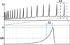 |
Fig. 1 Characteristic profile of quasi-periodic shockwave structures in an isentropically unstable medium showing gasdynamic disturbances. Here, A represents the pulse amplitude, L1 is the characteristic scale of the shockwave pulse, and L2 is the distance (period) between neighboring pulses. |
2 Model
To describe one-dimensional motion with velocity v along the x-axis in the atomic zone of a PDR, we consider the system of ideal gasdynamic equations supplemented by the generalized heat-loss function  . The governing equations are as follows:
 (1)
(1)
 (2)
(2)
 (3)
(3)
 (4)
(4)
In Equations (1)-(4), v, T, ρ, and P represent the velocity, temperature, density, and pressure, respectively. CV∞ is the heat capacity at constant volume, kB is the Boltzmann constant, m is the hydrogen atom mass. The notation d/dt = ∂/∂t + v ∂/∂x denotes the substantial derivative.
The generalized heat-loss function  is expressed as (Field 1965)
 (5)
(5)
where Λ(ρ, T) is the cooling rate and Γ(ρ, T) is the heating rate of the medium. The stationary condition is defined by equality of this function to zero  (ρ0, T0) = 0, which corresponds to thermal balance. Deviations from the stationary density and temperature parameters result in thermal misbalance. If thermal misbalance leads to increased heat release in high-pressure regions of an acoustic perturbation, the medium exhibits acoustic (isentropic) instability. Conversely, if thermal misbalance results in cooling in high-pressure regions, the acoustic disturbance is damped (Field 1965; Molevich & Oraevsky 1988).
As mentioned in Section 1, there are three types of thermal instability: isochoric, isobaric, and isentropic. These were initially described in terms of derivatives of the heat-loss function (see Field 1965, for details). Since we subsequently employ an analogy with a non-equilibrium relaxing medium, it is convenient to reformulate the instability conditions using the notations for the so-called low-frequency specific heat capacities at constant volume CV0 and pressure CP0 (6) and high- and low-frequency adiabatic indices, γ∞ and γ0, respectively (7) (see Molevich & Oraevsky 1988; Molevich et al. 2011 for details):
 (6)
(6)
 (7)
(7)
where CP∞ = CV∞ + kB/m is the specific heat capacity at constant pressure,  are partial derivatives of the generalized heat-loss function with respect to temperature and density, respectively, evaluated at the steady state. The conditions for thermal instability are summarized in Table 1.
With regard to the mechanism of heating in the PDR, it is noteworthy that this process is primarily driven by the photoelectric effect, which takes place on large polycyclic aromatic hydrocarbon (PAH) molecules and small dust particles.
FUV photons absorbed by grains produce energetic electrons. As these electrons diffuse through the grain, they lose energy via collisions. However, if, during this diffusion process, they reach the surface with sufficient energy, they can be injected into the gas phase with excess kinetic energy (Tielens 2005; Tielens & Hollenbach 1985). Under otherwise constant conditions, the photoelectric heating rate is proportional to the dust-to-gas mass ratio. For the Orion Bar PDR, the ratio of the dust abundance δd to that in the diffuse interstellar medium was assumed to be 1 for the standard model and 0.5 for an improved fit (Tielens & Hollenbach 1985). For PDRs with higher metallicity than that of the Orion Bar PDR, this can lead to a decrease in the characteristic heating time and a reduction in the characteristic size L1 of the forming nonlinear structures (Molevich & Riashchikov 2021). However, this linear increase in the photoelectric heating rate with dust-to-gas ratio only holds in the limit of low dust concentrations. At high dust densities, nonlinear corrections for dust grain charging and self-shielding become significant. According to Weingartner & Draine (2001), the size distribution of dust grains plays a crucial role. The grain size distributions are consistent with extinction curves characterized by parameters RV and bC, where RV is the ratio of visual extinction to reddening, and bC is the carbon abundance in the very small grains (radius ≤100 Å). The expression for the photoelectric heating rate in the atomic region of the PDR is given by (Weingartner & Draine 2001; Krasnobaev & Tagirova 2017) in the form
 (8)
(8)
where G0 is the ambient FUV flux field. For the Orion Bar PDR, G0 ranges from 2.2 × 10⁴ to 7.1 × 10⁴ H.U. (Habart et al. 2024). Here, ne represents the electron density in the medium, with ne = ξCn near the surface of PDR, where n = ρ/m and ξC is the carbon abundance in the gas. Quantities C0-6 are constants determined by the parameters RV, bC, grain size distribution, and radiation field spectrum, as detailed in Draine & Bertoldi (1996); Weingartner & Draine (2001). For our calculations, we adopt RV = 5.5 and bC = 3.0 × 10⁻⁵, consistent with Krasnobaev & Tagirova (2017).
There are mainly two processes that contribute to the cooling rate. Firstly, a significant part of the cooling in the medium is related to the collision of electrons with PAH and dust particles. According to Weingartner & Draine (2001), for temperature range T ≳ 1000 K, the cooling rate of the gas due to the accretion of electrons to grains can be calculated as follows:
 (9)
(9)
where  is in units of K1/2 cm3, D0-4 are constants determined by parameters RV and bC.
Second, cooling of the atomic gas of PDRs occurs mainly due to the excitation of fine-structure levels during collisions of atoms and ions of heavy elements with hydrogen atoms. The dominant contributions arise from the emission lines [CII] 158 µm, [OI] 63 µm, and [OI] 146 µm. The cooling rate due to radiative emission in general is expressed as
![Mathematical equation: \Lambda_{21} &= \xi E_{21} A_{21} \beta(\tau_{21})\\ &\quad\times\Big( m \big[ 1 + g_1/g_2 ~ \exp\left( E_{21} / k_B T \right) \left( 1 + \beta (\tau_{21}) n_{cr} / n \right) \big] \Big)^{-1},](/articles/aa/full_html/2025/09/aa54479-25/aa54479-25-eq15.png) (10)
(10)
where E21 is the energy difference between the upper level 2 and lower level 1 of some species, A21 is the probability of spontaneous transition, g1,2 are the statistical weights of two levels, ξ is the oxygen (ξO) or carbon (ξC) abundances, ncr = A21 /γ21 is the critical number density above which the levels undergo collisional thermalization, γ21 is the collisional de-excitation rate coefficient for atomic hydrogen collisions, β(τ21) is the escape probability at optical depth τ21 of the line. The values of the constants E21, A21, γ21 for the lines [CII] 158 µm, [OI] 63 µm, and [OI] 146 µm are given in Table 1 of (Krasnobaev & Tagirova 2017).
The atomic zone of the Orion Bar is characterized by the optical depths τ12 = τc, τo63, and τo146 for the lines [CII] 158 μm, [OI] 63 µm, and [OI] 146 µm, respectively. As shown in Krasnobaev & Tagirova (2017), optical depths τ12 can be expressed through the optical depth τc as τo63 = 0.72τc × ξO/ξC, τo146 = 0.92τ c × ξO/ξC. In the atomic zone of PDR, τc is usually in the range from 0 to 1 (Tielens 2005). The escape probability β = 0.5 at τc = 0 (near the boundary of PDR and the ionized gaz region). For this case, radiative cooling has its largest value. As τc increases, the value of β decreases.
By substituting ρ = mn, the heat-loss function can be expressed in terms of number density and temperature as  . Then, the generalized heat-loss function used in this study can be written in the following form (Krasnobaev & Tagirova 2017):
 (11)
(11)
The stationary state of medium is described by equation  , which allows us to estimate the stationary gas number density dependence on stationary temperature n0(T0). Figure 2 illustrates this dependence for different values of G0 and τc. Here, for certainty, we use abundances ξO = 2.56 × 10⁻⁴ and ξC = 1.2 × 10⁻⁴, as reported in (Wakelam & Herbst 2008). The influence of different values of ξO and ξC on n0(T0) is discussed in greater detail in Krasnobaev et al. (2016); Krasnobaev & Tagirova (2017); Riashchikov et al. (2022).
As can be clearly seen in the top panel of Figure 2, the stationary state is weakly dependent on the parameters G0. Therefore, for our subsequent numerical calculations, we adopt G0 = 4.0 × 10⁴, a commonly cited value in the literature Goicoechea et al. (2016); Salgado et al. (2016); Joblin et al. (2018); Habart et al. (2023, 2024). In contrast, the bottom panel of Figure 2 demonstrates a strong dependence of stationary parameters on optical depth τc. For cases where τc = 0.5, 0.75, 1.0, the resulting values of n0 align with the number density range nH = (0.5-1.0) × 105 cm−3, reported in Goicoechea et al. (2016); Salgado et al. (2016); Joblin et al. (2018); Habart et al. (2023, 2024).
Conditions for thermal instabilities based on low-frequency thermal capacities.
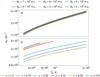 |
Fig. 2 Dependence of number density on temperature in the stationary state: a) with τc = 0.5 and different values of G0; b) with G0 = 4 × 10⁴ H.U. and different values of τc. |
3 Analytical and numerical approaches for shock waves description
In this study, we investigate the parameters of shock-wave structures that can form under conditions of isentropic instability. To achieve this, we employed both analytical and numerical approaches. The analytical methods, proposed in Zeldovich & Kompaneets (1960); Landau & Lifshitz (1987); Galimov & Molevich (2009), are used to describe wave properties during the linear and nonlinear stages of evolution. For further details on the analytical approach, refer to Section 3.1. Using these methods, we determine the amplitude A and width L1 of shock pulses (see Figure 1). However, the currently available analytical approaches do not provide complete information on the structures of interest. Therefore, we complement our study with numerical modeling to estimate the formation time of shock-wave structures and the period L2 between shock peaks. The numerical model is described in Section 3.2.
3.1 Analytical approach
To a first approximation, the growth time of wave structures can be estimated from the results of linear analysis. Within the linear approximation, wave properties are analyzed using the dispersion relation, which provides the conditions for wave amplification, growth rate, and phase speed.
To characterize the influence of heating and cooling processes, an analogy is drawn between heat-releasing and non-equilibrium relaxing media (Molevich & Oraevsky 1988; Molevich 2004; Molevich et al. 2011). Within this framework, the influence of the heat source is described using the previously introduced effective low-frequency heat capacities at constant volume CV0 and pressure CP0 (see Eq. (6)).
Thus, using the system of Equations (1)–(4) and the aforementioned notations, the dispersion relation for acoustic waves and the entropy mode can be expressed as
 (12)
(12)
Here, we use the characteristic cooling (heating) time:
 (13)
(13)
Representing the wave number as k = kRe + i kIm, and assuming kIm ≪ kRe, the increment kIm can be derived. This expression enables the analysis of the dependence of the wave growth time on its frequency:
 (14)
(14)
 (15)
(15)
In the presented equations, ξ is the effective bulk (second) viscosity coefficient caused by thermal misbalance, and ξ0 is the low-frequency bulk viscosity coefficient. The phase speed cph is given by
 (16)
(16)
where,  represent the high- (ωτ0 ≫ 1) and low-frequency (ωτ0 ≪ 1) limits of the phase speed of acoustic waves, respectively.
For wave amplification, the quantity kIm must be negative. It is clearly seen that the sign of kIm depends on the sign of bulk viscosity coefficient ξ. It can be shown that the condition for isentropic instability coincides with the condition for negative bulk viscosity, i.e., CV0 (γ∞ - γ0) < 0 (Molevich & Oraevsky 1988; Molevich et al. 2011). Thus, if the isentropic instability condition is satisfied (see Table 1), kIm is negative for all harmonics, leading to wave growth during the evolution of disturbances.
From Equations (14) and (15), we observe a quadratic dependence of the increment on frequency in the low-frequency limit. In contrast, the increment becomes frequency-independent in the high-frequency limit. The expressions for the increment in these limits are detailed in Molevich & Oraevsky (1988); Molevich et al. (2011). In Molevich et al. (2016), the frequency dependence of the damping and growth rates of magnetoacoustic waves is illustrated (see Figure 3 in cited article). The increment is smaller in the low-frequency limit but increases with frequency growth, eventually saturating at high frequencies. Consequently, in gasdynamic disturbances containing multiple harmonics, high-frequency harmonics contribute more significantly to the growth rate than low-frequency ones. Thus, the amplitude of disturbances with predominant high-frequency harmonics grow faster. This effect is further examined and confirmed in Section 4.
The maximum gain at a given wavelength occurs at a frequency (Kogan & Molevich 1986):
 (17)
(17)
or a timescale
 (18)
(18)
The parameter τq is employed below as a characteristic timescale for normalization purposes.
As the amplitude of the perturbation increases, the influence of nonlinear effects on its evolution becomes more pronounced. It has been shown in Molevich & Riashchikov (2021) that the analogy between heat-releasing and non-equilibrium relaxing media remains valid even in the nonlinear regime. In media with relaxation processes (Zeldovich & Kompaneets 1960; Landau & Lifshitz 1987; Galimov & Molevich 2009), a homogeneous stationary state is followed by a discontinuity of density, temperature, pressure, and gasdynamic velocity, which is sharp on the scale of the mean free path of particles. In the region behind the shock-wave front, slow relaxation processes of thermodynamic equilibrium establishment play an essential role. For this reason, the shock front is followed by a region of slower changes of gasdynamic quantities up to their equilibrium values. In media with thermal misbalance, the relaxation time is analogous to previously mentioned τ0, which is the time required to establish thermal balance between heating and cooling (see Equation (13)). This qualitative similarity of physical processes in the medium with thermal misbalance and relaxing media allows us to use this method to describe the profiles of stationary shock wave structures (Molevich & Riashchikov 2021). In the current paper, this method is denoted by the method of adiabats.
The foregoing method is designed to determine the type and properties of stationary structures in a medium with thermal misbalance. We should note that here, by the term “stationary wave structures”, we mean structures that do not change their shape over time in a reference frame moving with speed D. If we seek a solution to the system of Equations (1)–(4) in the form of one-dimensional stationary structures propagating through the medium at speed D, we can introduce the following automodel substitution z = x - Dt. We assume that the medium ahead of the wave front is undisturbed, with parameters ρ0, P0, T0, and that the initial velocity v0 = 0.
For stationary waves, integrating the system of Equations (1)–(4) in automodel form yields the following expressions (Molevich & Riashchikov 2021):
 (19)
(19)
 (20)
(20)
 (21)
(21)
 (22)
(22)
 (23)
(23)
where E is the specific energy.
The solution to the differential Equation (19) together with expressions (20)–(22) allows us to find the shape of the stationary structure propagating in the medium with thermal misbalance. However, if the stationary structure is a shock wave, these expressions can describe only the parameters of this structure behind the sharp front. This is because the thermodynamic parameters change so rapidly at the shock-wave discontinuity that heating and cooling processes do not have time to influence the jump conditions. Thus, variations in thermodynamic parameters directly at the shock front are governed by the Rankine–Hugoniot adiabat (24), a well-established concept in the theory of shock and detonation waves (Zeldovich & Kompaneets 1960):
 (24)
(24)
We also note that Equation (21) represents the well-known expression for the Rayleigh-Michelson line, whose slope in the PV-diagram is related to the propagation speed D of the structures. As shown in Molevich & Riashchikov (2021), the type of stationary structures depends on the order of intersection of the Rayleigh–Michelson line (21) with the curves describing the zeros of the numerator and denominator of Equation (19), as well as the Rankine–Hugoniot adiabat (24). This allowed the authors to describe possible types of stationary structures in isentropically stable and unstable media depending on their propagation speed D. In the case of an isentropically non-equilibrium medium, one of the structures described by Molevich & Riashchikov (2021) is the so-called autowave (self-sustained) pulse. An autowave pulse represents a self-sustaining nonlinear wave structure that maintains constant velocity and profile while propagating through the medium. Its velocity and amplitude are determined by the parameters of the propagation medium and the heat-loss function.
In this paper, we focus exclusively on expressions describing the parameters of the autowave pulse in an isentropically unstable medium, omitting other possible structures from consideration. This focus is justified for two reasons. First, the autowave pulse is the only possible stationary structure in an isentrop-ically unstable medium, characterized by identical parameters ahead of and behind the shock-wave discontinuity. Second, numerical experiments (see Section 4) show that initial perturbations of different shapes and amplitudes in a homogeneous medium consistently develop into a series of autowave pulses, with parameters that agree with the analytical predictions.
The autowave pulse represents a solution at which the derivative dρ/dz is positive everywhere along the Rayleigh-Michelson line (20). Such a solution is possible when it passes through the point of intersection of the zeros of the numerator and denominator of Eq. (19). Thus, the speed of pulse propagation Dp can be found from the solution of Equation (25):
 (25)
(25)
where

The density amplitude, ρA, of the autowave pulse is determined by the intersection condition of the Rayleigh–Michelson line (21) at D = Dp with the Rankine-Hugoniot adiabat (24) and is given by
 (26)
(26)
Using the calculated density value ρA , the amplitude values of temperature, pressure, and gasdynamic velocity at the shock front of the autowave pulse can be obtained from expressions (20)–(22).
As Equation (25) shows, the pulse speed Dp and, consequently, the pulse amplitude ρA are governed by the heat-loss function (5), i.e., by the medium’s properties. For a shockwave pulse, the amplitude decay behind the wavefront follows an approximately exponential profile (see Figure 4). Thus, to estimate the characteristic pulse width (L1, as shown in Figure 1), we measure the distance over which the magnitude behind the wavefront decreases by a factor of e.
The results obtained using this method are detailed in Section 4.1. Although this method has several advantages, it cannot provide information about the pulse growth time to its maximum amplitude or the distance L2 between the two following structures (Figure 1). To overcome these limitations, we use numerical modeling, as described in the following subsection.
3.2 Numerical model
As discussed in Section 3.1, the method of adiabats provides only the static shape of a single traveling structure. To evaluate the growth time of shockwave pulses and the period L2 between pulses, we use the Athena++ code (Stone et al. 2020) to numerically model the evolution of a hydrodynamic disturbance in the Orion Bar PDR. This code offers extensive possibilities for modeling hydrodynamic and magnetohydrodynamic processes.
We perform 1D simulations using the heat-loss function (11) and an initial perturbation described below. The center of the initial disturbance is located at x0 = 0. The density and pressure perturbations are modeled as Gaussian curves:
![Mathematical equation: a_{P,~\rho} = A_{P,~\rho} \exp{ \left[ \frac{-(x - x_0)^2}{\sigma^2} \right]},](/articles/aa/full_html/2025/09/aa54479-25/aa54479-25-eq36.png) (27)
(27)
where AP and Aρ are the amplitudes of the pressure and density perturbations, respectively, and σ is the characteristic spatial scale of the initial perturbation.
When performing calculations, the spatial coordinate was normalized to Lq :
 (28)
(28)
where τq is defined in Eq. (18).
The system of Equations (1)–(4) is solved using Low-dissipation Harten-Lax-van Leer-Contact (LHLLC) Riemann solver proposed by Minoshima & Miyoshi (2021). Time integration is performed using a second-order accurate van Leer predictor–corrector scheme. We use the outflow boundary conditions, as wave-boundary interactions are not the focus of this study. The Courant-Friedrichs-Lewy (CFL) number is set to 0.1 for all simulations.
Numerical calculations are subject to errors due to approximation in the numerical method, rounding errors, and other computational limitations. We generalize these effects of numerical modeling as numerical effects. The listed calculation errors may cause small disturbances on the surface of the modeled structure. As previously mentioned, disturbances with small characteristic sizes exhibit high growth rates. Consequently, such disturbances, even if they lack a physical origin, can grow into new shockwave pulses, complicating the analysis of the primary pulse’s growth. To prevent the occurrence of such disturbances, we performed our calculations with an additional isotropic viscosity coefficient µ = 0.01 (in the units used in Athena++). This additional viscosity suppresses small disturbances during the early stages of evolution, preventing them from interfering with the growth of the primary pulse. However, the inclusion of viscosity also has secondary effects: it reduces the amplitude of the main pulse and slightly increases its growth time. As a result, the amplitude obtained in numerical calculations is slightly lower than the theoretical prediction. Additionally, to isotropic viscosity, which we can supervise by coefficient µ, we have a viscosity, caused by listed numerical effects. The result of this viscosity presence is also a decrease of the amplitude of the pulse under study. For further details on the influence of additional viscosity caused by numerical effects on amplitude and methods to control this effect, see Appendix A.
The results of numerical modeling, presented in Sections 4.2–4.4, are compared with the analytical solutions described in Section 3.1 in terms of characteristic width and amplitude. The spatial grid step used in each numerical experiment is also provided.
Characteristic numerical values of the atomic zone of the Orion Bar PDR.
4 Results
4.1 Analytical estimation of shockwave pulse scale L1 and amplitudes
To begin, let us determine the conditions for isentropic instability in the Orion Bar for a chosen temperature T0, its corresponding concentration n0, and different values of optical thickness τc (see Figure 2).
We consider different values of optical depth, namely τc = 0.5, 0.75, and 1.0, and estimate the values of the low-frequency heat capacities CV0 and CP0 using Equation (6), with the previously chosen parameter values (see Table 2). The calculations reveal that the medium is always isochorically stable, i.e., CV0 > 0. Consequently, the condition for isentropic instability simplifies to the inequality γ0/γ∞ > 1. Figure 3 illustrates the dependence of the ratio γ0/γ∞ on temperature. It is evident that the condition for isentropic instability, as well as the values of the γ0/γ∞ ratio themselves, are basically independent of the optical depth τc . The medium becomes isentropically unstable at temperatures T0 ≳ 480 K.
Thus, gasdynamic perturbations in the Orion Bar, induced in regions with a stationary temperature T0 ≳ 480 K, can evolve into shock-wave pulses with amplitude of density ρA (26). For a known density amplitude ρA, the velocity amplitude vA and pressure amplitude PA in the shock-wave pulse are determined using Equations (20) and (21), respectively. These derived amplitudes ρA, PA, and vA, along with the pulse speed DP, are plotted in Figure 3 as functions of the stationary temperature T0.
Figure 3 shows that the pulse parameters mentioned above weakly depend on the optical depth τc. Due to this fact, for the certainty, we use the value τc = 0.5 in subsequent calculations. The parameters used for these calculations are summarized in Table 2.
Using the method of adiabats (Molevich & Riashchikov 2021), briefly described in Section 3.1, we obtain the pulse shape shown in Figure 4 for three temperature values: T0 = 600, 1000, and 2000 K. According to Figure 2, each temperature T0 corresponds to a specific stationary number density n0. The corresponding stationary values of T0, n0 are shown at the top of Figure 4 and in Table 3. This table also includes the pressure, velocity, and density amplitudes in the shock-wave pulses, as well as the ratio of the pulse propagation speed to the speed of sound DP/cs.
Figure 4 shows that in spite of completely different medium parameters (T0 and n0) and pulse parameters (including amplitudes ρA, PA, vA and propagation velocity DP), their characteristic spatial scale remains practically unchanged. We investigated the temperature dependence of the characteristic scale L1, defined as the distance over which the density magnitude behind the wavefront decreases by a factor of e, in the range of 600–2000 K (see Figure 5). One can see that the values of L1 range from 8.43 × 10 4 to 8.87 × 10 4 pc, which is comparable to the sizes of observed substructures in the Orion Bar PDR, with widths of 1″-2″ (i.e., 0.002-0.004 pc) (Habart et al. 2023, 2024; Peeters et al. 2024).
While the shape of the shockwave pulse, determined by its amplitude and characteristic scale L1, can be derived analytically, the period L2 of the quasi-periodic structure (see Figure 1) requires numerical modeling of the evolution of initial disturbances occurring in the medium with the stationary state defined as (n0, T0). Therefore, in Section 4.2, we numerically simulate the process of pulse formation from the initial perturbation and estimate the parameters L1 and L2 during the early stages of pulse evolution. Subsequently, in Section 4.3, we numerically analyze the final stage of the pulse evolution, enabling us to demonstrate its autowave nature and estimate the parameter L2. Finally, in Section 4.4, we evaluate the pulse formation time for various initial perturbations.
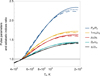 |
Fig. 3 Dependence of adiabatic indices ratio, γ0/γ∞, and pulse parameters on the steady state temperature, T0, of Orion Bar PDR. Calculations are shown for different values of optical depth: τc = 0.5 (solid line), τc = 0.75 (dashed line), τc = 1.0 (dot-dashed line). The gray thin line, γ0/γ∞ = 1, divides the figure into two regions. The upper region corresponds to isentropic instability, while the lower region indicates stability. Shock-wave pulses occur where γ0/γ∞ > 1, i.e., T0 ≳ 480 K. |
Values of pressure, velocity, and density amplitudes and a pulse propagating velocity obtained by the method of adiabats for characteristic temperatures and number densities in the atomic region of the Orion Bar PDR.
4.2 Investigating early stages of pulse evolution
In this section, we describe the formation of a sequence of shock-wave structures from an initial perturbation. Here, for definiteness, we assume the initial perturbation to be a Gaussian function (27) with amplitude of Aρ = 0.1, characteristic width of σ = 0.1 Lq, and adiabatic amplitude ratio of Ap/Aρ = γ∞ = 5/3.
The evolution of the pulses is illustrated in Figure 6. Over a timescale of roughly 10 000 years, a multifront structure with sharp gas-dynamic disturbance fronts develops. However, during this time, none of the pulses reach their maximum amplitude. The interval between the first and second maxima in the pulses is measured as L2 = 6.0 × 10⁻³ pc. The characteristic scale of the first pulse, which exhibits the most advanced development, is L1 = 9.0 × 10⁻⁴ pc. This scale aligns closely with the analytically derived pulse scales, which is shown in Figure 5.
During the initial 9600 years, the first pulse propagates a distance of approximately 4.0 × 10⁻² pc from the starting point. This distance is consistent with the estimated separation between the IF and DF in the Orion Bar PDR, as reported in previous studies (Salgado et al. 2016; Habart et al. 2023, 2024). Thus, if wave reflection from the fronts is neglected and only the evolution of a single initial perturbation is considered, a maximum of three shock-wave fronts can form within the investigated scale. However, it is important to note that wave fronts can propagate not only perpendicular to the IF but also parallel to it (e.g., Salgado et al. (2016) estimates the characteristic length of the PDR along the IF as ≈0.32 pc) or at an angle. Additionally, re-reflection within the medium is plausible, which could allow perturbations to develop into larger amplitudes. In this context, the autowave nature of these pulses becomes significant, particularly their ability to retain their shape after interacting with similar structures.
4.3 Discussing autowave nature of shockwave pulses
In this section, we investigate and demonstrate the autowave (self-sustained) nature of the studied shock-wave structures through numerical modeling. The results are derived using the computational approach described in Section 3.2. Verification of the numerical calculations against the analytical model is provided in Appendix A.
We now proceed to demonstrate the autowave nature of the studied structures on longer evolutionary timescales. As a fundamental example of an initial perturbation, we again employ the Gaussian function (27). To illustrate that the parameters of the resulting structures remain invariant regardless of the initial perturbation, we examined various types of initial perturbations, including different density and pressure amplitude ratios AP/Aρ, characteristic widths σ, and absolute density amplitude values Aρ. Due to the autowave nature of the structures, the pattern at later stages of evolution exhibits minimal variation when altering different parameters of the initial perturbation. To avoid redundancy and ensure clarity in the manuscript, we present only the modeling results corresponding to variations in the initial perturbation width σ. For consistency across all calculations, we selected an adiabatic initial perturbation (AP/Aρ = 5/3) with an initial density amplitude of Aρ = 0.05.
The results of our numerical simulations are presented in Figure 7. For these calculations, we used width values of σ = (0.1, 0.5, 1.0, 3.0) Lq. The curves in this figure depict the state of the medium after the evolution of the initial perturbation over a timescale of τ = 140 thousand years. By this time, the pulse amplitudes have reached maximum stationary value, which is predicted by Equation (26). It is evident that, in all cases, the evolution of the initial perturbation leads to the formation of autowave (self-sustained) structures with identical amplitudes. Furthermore, the period of fully developed pulses (whose “tails” have reached a steady-state level) is approximately the same across all calculations, with L2 ≈ (2.14 ± 0.06) × 10−2 pc.
It is noteworthy that the number of fully developed autowave structures at the same moment τ after the disturbance occurrence varies depending on the initial perturbation width. Specifically, for σ = 3.0 Lq, only the first two pulses have fully developed. In contrast, for other initial perturbation widths, three autowave pulses have already fully formed by the same time. For the case of σ = 3.0 Lq, the third autowave pulse will fully develop by τ = 175 thousand years after the onset of evolution.
Based on the presented results, we conclude that the width σ of the initial perturbation does not influence the amplitude of the resulting structures. However, the width σ of the initial perturbation does affect both the formation time to the final amplitude of the first (or leading) pulse and the time to form a sequence of the same given number of fully developed pulses. This effect is related to the previously discussed frequency dependence of the acoustic wave increment, as described by expressions (14) and (15). High-frequency harmonics, due to their larger increment, contribute more significantly to the amplitude growth of the overall structure compared to low-frequency harmonics. Consequently, perturbations with smaller characteristic widths σ, which are dominated by high frequencies, evolve more rapidly than those with larger σ values. This results in variations in the time required to establish the periods between pulses and the amplitude of the leading pulse, as is detailed in the subsequent analysis.
To estimate the minimum time required for the leading pulse to reach its maximum amplitude, we conducted a series of experiments with varying initial perturbation parameters. The results of these experiments, along with a visualization of the leading pulse amplitude growth over time, are presented in the following subsection.
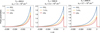 |
Fig. 4 Perturbation profiles of pressure, velocity, and density in the shock-wave pulse obtained for stationary states by the method of adiabats at different temperatures and number densities. The point of the pulse front is selected as the null-point. |
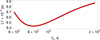 |
Fig. 5 Dependence of pulse characteristic scale, L1, on stationary temperature, T0. |
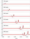 |
Fig. 6 Profiles of the structures formed at different moments of time, τ, after the beginning of evolution from Gaussian initial disturbance with parameters Aρ = 0.1, σ = 0.1 Lq, AP/Aρ = 5/3. |
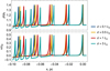 |
Fig. 7 Comparison of the shape and size of structures for density and velocity, obtained using different characteristic widths, σ, of the initial disturbance. The point of the leading pulse front is selected as the null-point. |
4.4 Estimating pulse formation time
To investigate the pulse formation time, we selected the width σ, the initial amplitude Aρ, and the ratio AP/Aρ as the variable parameters of the initial perturbation, which is described by Equation (27).
To further explore the spectral composition of the initial perturbation and its influence on the growth dynamics of the self-sustained pulse, as introduced in the preceding subsection, a series of numerical experiments was conducted by varying the characteristic width σ of the initial pulse. The results of these simulations, corresponding to different values of σ, are illustrated in panel a of Figure 8.
For this set of experiments, the initial amplitude Aρ was set to 0.1, and the ratio AP/Aρ was maintained at 5/3. The results demonstrate that the time required to attain the stationary amplitude is significantly influenced by the width of the initial perturbation. Moreover, the evolution of the perturbation can be divided into two distinct stages: linear and nonlinear. Taking into account the calculated values of the pulse amplitudes, we roughly define the linear stage as the period during which the perturbation grows to half of its maximum amplitude, while the nonlinear stage encompasses the subsequent time interval until the stationary state is reached. It is evident that the linear stage of the process is accurately described by the previously discussed frequency dependence of the wave increment (see Equation (14)). Specifically, perturbations exhibiting a larger width (or period) require a longer duration to develop. For instance, a perturbation with a width ofσ = 3.0 Lq attains half of its maximum amplitude in ≈25 000 years, whereas a perturbation with a width of σ = 0.1 Lq reaches the same amplitude threshold in ≈5000 years. Further, during the nonlinear stage, the time required to achieve amplitudes approaching the stationary value is approximately consistent, on the order of 104 years. Notably, the total time required to reach the stationary amplitude value does not exceed 35 000 years, which does not exceed the estimated lifetime of the Orion Bar PDR, approximately 105 years, as estimated by Salgado et al. (2016); Kirsanova & Wiebe (2019).
In addition, the influence of the initial disturbance amplitude Aρ was investigated in numerical simulations. The simulation results are shown in panel b of Figure 8. For this set of experiments, the width σ was set to 0.1 Lq, and the ratio AP/Aρ was also maintained at 5/3. It is evident that for small amplitudes Aρ ≪ 1, an increase in the initial amplitude leads to a predictable reduction in the time required to transition to the nonlinear stage. For initial perturbations with high amplitudes Aρ ⩾ 1, the nonlinear stage commences immediately upon induction and is characterized by a rapid decline in the maximum value followed by a gradual approach to the stationary amplitude of the autowave pulse.
In the final set of numerical simulations, the impact of varying types of initial perturbations was analyzed by examining different values of AP/Aρ. The characteristic width was kept the same as in the previous series (σ = 0.1Lq), and both weak (Aρ = 0.1) and strong (Aρ = 1.0) initial perturbations were considered. The results are shown in panel c of Figure 8. They confirm the conclusions outlined earlier and further demonstrate that the growth duration depends only minimally on the ratio of specific initial amplitudes.
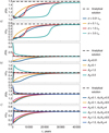 |
Fig. 8 Dynamics of the maximum pulse amplitude for density and velocity compared with the static analytical solution of the pulse amplitude. (a) Dynamics obtained with different initial disturbance characteristic widths σ. (b) Dynamics obtained with different initial disturbance density amplitude Aρ. (c) Dynamics obtained with different initial disturbance pressure to density amplitude ratio AP/Aρ in two characteristic cases: Aρ = 0.1 (low amplitude) and Aρ = 1.0 (high amplitude). |
5 Discussion
The study of the Orion Bar PDR as an isentropically unstable medium presented in current work has provided valuable insights into the formation and evolution of shockwave structures in PDRs. By combining analytical and numerical approaches, we have been able to model the nonlinear dynamics of these structures and compare our results with observational data from various telescopes, including ALMA, Herschel, Keck, and the James Webb Space Telescope (JWST). Our findings contribute to the broader understanding of the physical processes governing the interstellar medium and the role of thermal instabilities in shaping its structure.
The Orion Bar PDR, being one of the closest and most well-studied PDRs, serves as an ideal laboratory for investigating the interplay between FUV radiation from massive stars and the surrounding interstellar gas. Observations from ALMA, Herschel Space Observatory and JWST have revealed a wealth of substructures, including filaments, ridges, and globules, with characteristic sizes ranging from a few arcseconds to sub-arcsecond scales (Goicoechea et al. 2016; Joblin et al. 2018; Habart et al. 2023, 2024; Peeters et al. 2024). These structures are often associated with non-thermal gas motions, suggesting the presence of dynamic processes such as shockwaves and turbulence.
Our theoretical framework, based on the isentropic instability model (Oppenheimer 1977; Molevich et al. 2011; Krasnobaev et al. 2016; Krasnobaev & Tagirova 2017, 2019; Zavershinskii et al. 2020; Molevich & Riashchikov 2021; Riashchikov et al. 2022), provides a plausible explanation for the observed phenomena. Unlike isobaric instability, which leads to the formation of static condensations, isentropic instability results in the amplification of acoustic waves, leading to the propagation of shockwave pulses through the medium. This model aligns well with the observed dynamic structures in the Orion Bar, particularly in the atomic zone, where non-thermal velocities and periodic density enhancements have been detected.
One of the key findings of our study is the close correspondence between the predicted shockwave parameters and the observed characteristics of the Orion Bar PDR. The velocity amplitude of the shockwave pulses, calculated to be approximately vA = 0.72 cS for T0 = 2000 K (see Table 3), is consistent with the non-thermal velocity estimates vnth = 0.49 cS for T0 = 2000 K derived from spectral line broadening observed in the Orion Nebula (Ferland et al. 2012). This agreement suggests that the isentropic instability model provides a plausible explanation for the observed non-thermal motions in the atomic zone.
Furthermore, the characteristic scales L1 and L2 of the shockwave pulses are in good agreement with observational data. Specifically, the characteristic width of the shockwave pulse L1, found to be approximately ~0.001 pc, matches the observed widths of dense structures in the Orion Bar, which range from 1″ to 2″ (approximately 0.002 to 0.004 pc) (Habart et al. 2023, 2024; Peeters et al. 2024). Additionally, the period of the pulses L2, estimated as ~0.02 pc, aligns with the observed spacing between substructures in the DF. Observations of the Orion Bar PDR reveal that substructures, such as ridges and filaments, are spaced at roughly periodic intervals of about 5″ (0.01 pc). This spacing is consistent with the calculated L2 value, suggesting that the quasi-periodic nature of the shockwave structures could account for the observed spacing between dense substructures in the PDR.
These results demonstrate that the isentropic instability model can successfully reproduce the spatial characteristics of the filamentary and reticulate structures observed in the Orion Bar PDR. The agreement between the model predictions and observational data underscores the model’s potential to explain the formation and dynamics of substructures in PDRs.
Our numerical simulations have also revealed that the time required for the leading shockwave pulse to reach its maximum amplitude ranges from 5000 to 40 000 years, depending on the initial perturbation parameters. This timescale is well within the estimated lifetime of the Orion Bar PDR, which is approximately 105 years (Salgado et al. 2016; Kirsanova & Wiebe 2019). This suggests that the observed substructures could have formed and evolved within the current lifetime of the Orion Bar. However, it is important to note that the time required to establish a long sequence of fully developed pulses may exceed the lifetime of the Orion Bar. This implies that the observed substructures may have originated from initial perturbations with relatively small characteristic widths, which evolve more rapidly due to the higher increment of high-frequency harmonics. This finding underscores the importance of considering the spectral composition of initial perturbations when modeling the evolution of shockwave structures in PDRs.
While our model offers a plausible explanation for many of the observed features in the Orion Bar PDR, certain discrepancies remain that necessitate further investigation. As reported by Joblin et al. (2018); Habart et al. (2024); Peeters et al. (2024), the observed background number density values in the atomic zone of the Orion Bar PDR fall within the range of nH = (0.5-1.0) × 105 cm−3. In contrast, our estimates for the stationary-state number density yield values in the range of n = (0.6-4.0) × 105 cm−3. These estimates were derived based on currently available models describing the heating and cooling mechanisms of the Orion Bar PDR. The observed disparity between the empirical data and our model predictions is likely attributable to the limitations of existing models in accurately capturing nonadiabatic processes. Specifically, the discrepancy suggests that incorporating additional physical processes – such as cooling via [CI] lines (Tielens 2005), cosmic ray heating (Kirsanova & Wiebe 2019), or more intricate kinetic processes (particularly near the DF) (Röllig & Ossenkopf-Okada 2022) – into the heat-loss function may be necessary to achieve a more precise representation of the observed conditions. Further refinement of these models is essential to reconcile theoretical predictions with observational data and to advance our understanding of the complex physical processes governing PDRs.
Moreover, the current model assumes a one-dimensional geometry, which may not fully capture the complexity of the three-dimensional structures observed in the Orion Bar. Future studies could benefit from extending the model to include multidimensional effects, as well as incorporating additional heating and cooling mechanisms that are relevant to the interstellar medium. While our analysis has focused on isentropic instability mechanisms, we note that alternative fragmentation processes may operate in the molecular cloud. In particular, large-scale instabilities such as the Vishniac instability in expanding shells (Vishniac 1983) and thin-shell gravitational instabilities (Elmegreen 1994) typically operate on larger scales (>0.1 pc), potentially contributing (if applicable under Orion Bar conditions) to the molecular cloud’s large-scale structure. Additionally, turbulence-driven fragmentation under isentropic instability conditions may produce an additional hierarchy of scales that will be investigated in forthcoming work.
In conclusion, our study demonstrates that the isentropic instability model provides a robust framework for understanding the formation and evolution of shockwave structures in the atomic zone of the Orion Bar PDR. The close agreement between the predicted and observed parameters of these structures supports the hypothesis that isentropic instability plays a key role in shaping the observed substructures in PDRs. However, further refinements to the model, including the incorporation of additional physical processes and multidimensional effects, will be necessary to fully reconcile the theoretical predictions with the observational data.
The insights gained from this study not only enhance our understanding of the Orion Bar PDR but also have broader implications for the study of other PDRs and the interstellar medium in general. As observational capabilities continue to improve, particularly with the advent of next-generation telescopes such as JWST, we can expect to uncover even more detailed and complex structures in PDRs, providing further opportunities to test and refine our theoretical models.
Acknowledgements
Acknowledgements. This work was supported in part by the Ministry of Science and Higher Education of the Russian Federation under State assignment to educational and research institutions under Project No. FSSS-2023-0009 and FFMR-2024-0017. We also acknowledge the use of data from ALMA, Herschel, Keck, and JWST, which have been instrumental in advancing our understanding of the Orion Bar PDR.
Appendix A Comparison of numerical and analytical solutions
We consider that it is important to conduct a comparative analysis of amplitudes and characteristic scale L1, which are obtained by numerical modeling performed with the approach described in Section 3.2, and analytical solution of equations presented in Section 3.1.
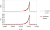 |
Fig. A.1 A shockwave pulse shape modeled by numerical calculation compared with an autowave pulse obtained by analytical method for density and velocity. The stationary parameters of the medium are T0 = 1000 K, n0 = 2.2 × 105 cm−3. |
Figure A.1 shows a shape of a shockwave pulse obtained in numerical solution of equations (1) - (4) (red curve) at the moment of time τ = 44 thousand years after the appearance of the initial perturbation (27). The parameters of the medium are given in Table 2. To test the numerical scheme, Figure A.1 also shows the same pulse (dashed curve) obtained analytically. It can be seen that the two pulses are almost identical. The characteristic scale obtained by numerical method L1 = 8.98 × 10⁻⁴ pc is approximately equal to the analytical value discussed in the Section 4.1.
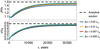 |
Fig. A.2 Dynamic of maximum pulse amplitude for density and velocity compared with the static analytical solution of the pulse amplitude for different spatial size of grid cells ∆x = (0.5 - 2.0) × 10−2Lq. Parameters of the initial perturbation are Aρ = 0.1, σ = 0.1 Lq, AP/Aρ = 5/3. |
Presented numerical experiments have shown us an equality of pulse amplitude and width for analytical and numerical methods, which makes the two methods relevant for the further studies. However, the pulse amplitude in numerical simulation is somewhat smaller than in the analytical solution. The effect of the amplitude decrease is caused by the presence of the additional viscosity of the numerical method itself (see Section 3.2). The effect can be reduced by decreasing the spatial cell size ∆x.
The influence of grid step on the maximum pulse amplitude is shown in Figure A.2. The results, which are presented in Figure A.1 and in Sections 4.3, 4.4, are obtained with the spatial grid step ∆x = 5 × 10⁻³ Lq.
References
- Abergel, A., Misselt, K., Gordon, K., et al. 2024, A&A, 687, A4 [NASA ADS] [CrossRef] [EDP Sciences] [Google Scholar]
- Claes, N., & Keppens, R. 2019, A&A, 624, A96 [NASA ADS] [CrossRef] [EDP Sciences] [Google Scholar]
- Downes, T. P., Hartigan, P., & Isella, A. 2023, MNRAS, 519, 5427 [Google Scholar]
- Draine, B. T., & Bertoldi, F. 1996, ApJ, 468, 269 [Google Scholar]
- Dudorov, A. E., Stepanov, C. E., Fomin, S. O., & Khaibrakhmanov, S. A. 2019, MNRAS, 487, 942 [Google Scholar]
- Elmegreen, B. G. 1994, ApJ, 427, 384 [Google Scholar]
- Ferland, G. J., Henney, W., O’Dell, C., et al. 2012, ApJ, 757, 79 [NASA ADS] [CrossRef] [Google Scholar]
- Field, G. B. 1965, ApJ, 142, 531 [Google Scholar]
- Flannery, B. P., & Press, W. H. 1979, ApJ, 231, 688 [Google Scholar]
- Fragile, P. C., Etheridge, S. M., Anninos, P., Mishra, B., & Kluz´niak, W. 2018, ApJ, 857, 1 [CrossRef] [Google Scholar]
- Galimov, R., & Molevich, N. 2009, Fluid Dyn., 44, 158 [Google Scholar]
- Goicoechea, J., Pety, J., Cuadrado, S., et al. 2016, Nature, 537, 207 [CrossRef] [Google Scholar]
- Goldsmith, D., Habing, H., & Field, G. 1969, ApJ, 158, 173 [Google Scholar]
- Habart, E., Gal, R. L., Alvarez, C., et al. 2023, A&A, 673, A15 [NASA ADS] [CrossRef] [EDP Sciences] [Google Scholar]
- Habart, E., Peeters, E., Berné, O., et al. 2024, A&A, 685, A73 [NASA ADS] [CrossRef] [EDP Sciences] [Google Scholar]
- Hartigan, P., Downes, T., & Isella, A. 2020, ApJ, 902, L1 [NASA ADS] [CrossRef] [Google Scholar]
- Hartigan, P., Hummel, M., Isella, A., & Downes, T. 2022, ApJ, 164, 257 [Google Scholar]
- Ibanez, S. M. H., & Sanchez, D. N. M. 1992, ApJ, 396, 717 [Google Scholar]
- Jennings, R. M., & Li, Y. 2021, MNRAS, 505, 5238 [NASA ADS] [CrossRef] [Google Scholar]
- Ji, S., Oh, S. P., & McCourt, M. 2018, MNRAS, 476, 852 [NASA ADS] [CrossRef] [Google Scholar]
- Joblin, C., Bron, E., Pinto, C., et al. 2018, A&A, 615, A129 [NASA ADS] [CrossRef] [EDP Sciences] [Google Scholar]
- Kirsanova, M. S., & Wiebe, D. S. 2019, MNRAS, 486, 2525 [CrossRef] [Google Scholar]
- Kogan, E. Y., & Molevich, N. 1986, Sov. Phys. J., 29, 547 [Google Scholar]
- Krasnobaev, K. 2000, Ap&SS, 274, 307 [Google Scholar]
- Krasnobaev, K., & Tarev, V. Y. 1987, Astron. Rep., 64, 1210 [Google Scholar]
- Krasnobaev, K. V., & Tagirova, R. R. 2017, MNRAS, 469, 1403 [NASA ADS] [CrossRef] [Google Scholar]
- Krasnobaev, K., & Tagirova, R. 2019, Astron. Lett., 45, 147 [Google Scholar]
- Krasnobaev, K., Tagirova, R., Arafailov, S., & Kotova, G. Y. 2016, Astron. Lett., 42, 460 [NASA ADS] [CrossRef] [Google Scholar]
- Landau, L. D., & Lifshitz, E. M. 1987, Fluid Mechanics, 2nd edn., 6, Course of Theoretical physics, Eds. L. D. Landau, & E. M. Lifshitz (Butterworth-Heinemann) [Google Scholar]
- Lis, D., & Schilke, P. 2003, ApJ, 597, L145 [NASA ADS] [CrossRef] [Google Scholar]
- Minoshima, T., & Miyoshi, T. 2021, J. Computat. Phys., 446, 110639 [NASA ADS] [CrossRef] [Google Scholar]
- Molevich, N. 2004, in 42nd AIAA Aerospace Sciences Meeting and Exhibit, 1020 [Google Scholar]
- Molevich, N., & Oraevsky, A. 1988, J. Exp. Theor. Phys., 67, 504 [Google Scholar]
- Molevich, N., & Riashchikov, D. 2021, Phys. Fluids, 33 [Google Scholar]
- Molevich, N., Zavershinsky, D., Galimov, R., & Makaryan, V. 2011, Ap&SS, 334, 35 [Google Scholar]
- Molevich, N., Ryashchikov, D., & Zavershinskiy, D. 2016, Magnetohydrodynamics, 52, 199 [Google Scholar]
- Molevich, N., Zavershinskiy, D., & Ryashchikov, D. 2016, Magnetohydrodynamics, 52, 191 [Google Scholar]
- Nakariakov, V. M., Mendoza-Briceño, C. A., et al. 2000, ApJ, 528, 767 [NASA ADS] [CrossRef] [Google Scholar]
- Oppenheimer, M. 1977, ApJ, 211, 400 [Google Scholar]
- Owl, R. C. Y., Meixner, M. M., Wolfire, M., Tielens, A., & Tauber, J. 2000, ApJ, 540, 886 [Google Scholar]
- Parikh, M. K., & Wilczek, F. 1998, Phys. Rev. D, 58, 064011 [Google Scholar]
- Parker, E. N. 1953, ApJ, 117, 431 [Google Scholar]
- Peeters, E., Habart, E., Berné, O., et al. 2024, A&A, 685, A74 [NASA ADS] [CrossRef] [EDP Sciences] [Google Scholar]
- Peng, C.-H., & Matsumoto, R. 2017, ApJ, 836, 149 [Google Scholar]
- Priest, E., & Smith, E. 1979, Sol. Phys., 64, 267 [NASA ADS] [CrossRef] [Google Scholar]
- Riashchikov, D. S., Pomelnikov, I. A., & Molevich, N. E. 2022, Bull. Lebedev Phys. Inst., 49, 307 [NASA ADS] [CrossRef] [Google Scholar]
- Röllig, M., & Ossenkopf-Okada, V. 2022, A&A, 664, A67 [NASA ADS] [CrossRef] [EDP Sciences] [Google Scholar]
- Salgado, F., Berné, O., Adams, J. D., et al. 2016, ApJ, 830, 118 [Google Scholar]
- Smith, E., & Priest, E. 1977, Sol. Phys., 53, 25 [NASA ADS] [CrossRef] [Google Scholar]
- Stone, J. M., Tomida, K., White, C. J., & Felker, K. G. 2020, ApJS, 249, 4 [NASA ADS] [CrossRef] [Google Scholar]
- Suleimenov, I., Aushev, V., Tulebekov, E., & Antoshchuk, I. 2006, Geomagn. Aeron., 46, 371 [Google Scholar]
- Tielens, A. 2005, The Physics and Chemistry of the Interstellar Medium (Cambridge University Press) [Google Scholar]
- Tielens, A., & Hollenbach, D. 1985, ApJ, 291, 722 [NASA ADS] [CrossRef] [Google Scholar]
- Vishniac, E. T. 1983, ApJ, 274, 152 [NASA ADS] [CrossRef] [Google Scholar]
- Wakelam, V., & Herbst, E. 2008, ApJ, 680, 371 [NASA ADS] [CrossRef] [Google Scholar]
- Wareing, C., Pittard, J., Falle, S., & Van Loo, S. 2016, MNRAS, 459, 1803 [NASA ADS] [CrossRef] [Google Scholar]
- Weingartner, J. C., & Draine, B. T. 2001, ApJS, 134, 263 [CrossRef] [Google Scholar]
- Wu, R., Bron, E., Onaka, T., et al. 2018, A&A, 618, A53 [NASA ADS] [CrossRef] [EDP Sciences] [Google Scholar]
- Xia, C., & Keppens, R. 2016, ApJ, 825, L29 [NASA ADS] [CrossRef] [Google Scholar]
- Zanstra, H. 1955, Vistas Astron., 1, 256 [Google Scholar]
- Zavershinskii, D., Kolotkov, D., Nakariakov, V. M., Molevich, N., & Ryashchikov, D. 2019, Phys. Plasmas, 26 [Google Scholar]
- Zavershinskii, D., Molevich, N., Riashchikov, D., & Belov, S. 2020, Phys. Rev. E, 101, 043204 [Google Scholar]
- Zeldovich, I. B., & Kompaneets, A. S. 1960, in Theory of Detonation [Google Scholar]
- Zemlyanukha, P., Zinchenko, I. I., Dombek, E., et al. 2022, MNRAS, 515, 2445 [Google Scholar]
All Tables
Values of pressure, velocity, and density amplitudes and a pulse propagating velocity obtained by the method of adiabats for characteristic temperatures and number densities in the atomic region of the Orion Bar PDR.
All Figures
|
Fig. 1 Characteristic profile of quasi-periodic shockwave structures in an isentropically unstable medium showing gasdynamic disturbances. Here, A represents the pulse amplitude, L1 is the characteristic scale of the shockwave pulse, and L2 is the distance (period) between neighboring pulses. |
| In the text | |
|
Fig. 2 Dependence of number density on temperature in the stationary state: a) with τc = 0.5 and different values of G0; b) with G0 = 4 × 10⁴ H.U. and different values of τc. |
| In the text | |
|
Fig. 3 Dependence of adiabatic indices ratio, γ0/γ∞, and pulse parameters on the steady state temperature, T0, of Orion Bar PDR. Calculations are shown for different values of optical depth: τc = 0.5 (solid line), τc = 0.75 (dashed line), τc = 1.0 (dot-dashed line). The gray thin line, γ0/γ∞ = 1, divides the figure into two regions. The upper region corresponds to isentropic instability, while the lower region indicates stability. Shock-wave pulses occur where γ0/γ∞ > 1, i.e., T0 ≳ 480 K. |
| In the text | |
|
Fig. 4 Perturbation profiles of pressure, velocity, and density in the shock-wave pulse obtained for stationary states by the method of adiabats at different temperatures and number densities. The point of the pulse front is selected as the null-point. |
| In the text | |
|
Fig. 5 Dependence of pulse characteristic scale, L1, on stationary temperature, T0. |
| In the text | |
|
Fig. 6 Profiles of the structures formed at different moments of time, τ, after the beginning of evolution from Gaussian initial disturbance with parameters Aρ = 0.1, σ = 0.1 Lq, AP/Aρ = 5/3. |
| In the text | |
|
Fig. 7 Comparison of the shape and size of structures for density and velocity, obtained using different characteristic widths, σ, of the initial disturbance. The point of the leading pulse front is selected as the null-point. |
| In the text | |
|
Fig. 8 Dynamics of the maximum pulse amplitude for density and velocity compared with the static analytical solution of the pulse amplitude. (a) Dynamics obtained with different initial disturbance characteristic widths σ. (b) Dynamics obtained with different initial disturbance density amplitude Aρ. (c) Dynamics obtained with different initial disturbance pressure to density amplitude ratio AP/Aρ in two characteristic cases: Aρ = 0.1 (low amplitude) and Aρ = 1.0 (high amplitude). |
| In the text | |
|
Fig. A.1 A shockwave pulse shape modeled by numerical calculation compared with an autowave pulse obtained by analytical method for density and velocity. The stationary parameters of the medium are T0 = 1000 K, n0 = 2.2 × 105 cm−3. |
| In the text | |
|
Fig. A.2 Dynamic of maximum pulse amplitude for density and velocity compared with the static analytical solution of the pulse amplitude for different spatial size of grid cells ∆x = (0.5 - 2.0) × 10−2Lq. Parameters of the initial perturbation are Aρ = 0.1, σ = 0.1 Lq, AP/Aρ = 5/3. |
| In the text | |
Current usage metrics show cumulative count of Article Views (full-text article views including HTML views, PDF and ePub downloads, according to the available data) and Abstracts Views on Vision4Press platform.
Data correspond to usage on the plateform after 2015. The current usage metrics is available 48-96 hours after online publication and is updated daily on week days.
Initial download of the metrics may take a while.