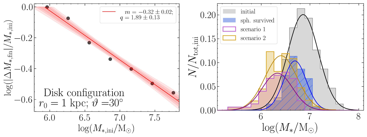
Left panel: Fraction of the clump mass lost after 9.23 Gyr |ΔM_*, fin|/M_*, ini as a function of the initial mass M_*, ini. Here ΔM_*, fin = M_*, fin(4r_s)−M_*, ini, where M_*, fin(4r_s) is the final mass within four initial Plummer scale radii, computed as in Sect. 5.2. The circles are the results from the simulations of resolved clumps described in Sect. 5.2, while the line is the best fit (Eq. 17) and the shaded area is the 1σ interval. Right panel: Distributions of the number of clumps per mass bin, normalised to the total initial number of clumps. The grey and blue histograms are the analogues of those shown in the bottom panel of Fig. 7, and they show the initial and surviving number of clumps, respectively, in the spherical configuration case considering the effects of dynamical friction only. The purple histogram shows the mass distribution of the surviving clumps of scenario 1 (short dynamical-friction timescale; Sect. 5.2), while the golden histogram shows the mass distribution of the surviving clumps of scenario 2 (short tidal-stripping timescale; Sect. 5.2). A Gaussian function is fitted to each histogram and shown with the corresponding colour.