| Issue |
A&A
Volume 701, September 2025
|
|
|---|---|---|
| Article Number | A129 | |
| Number of page(s) | 21 | |
| Section | Extragalactic astronomy | |
| DOI | https://doi.org/10.1051/0004-6361/202554669 | |
| Published online | 05 September 2025 | |
The dynamical evolution of the stellar clumps in the Sparkler galaxy
1
Dipartimento di Fisica e Astronomia “Augusto Righi”, Università di Bologna, Via Piero Gobetti 93/2, I-40129 Bologna, Italy
2
The Oskar Klein Centre, Department of Astronomy, Stockholm University, AlbaNova, SE-10691 Stockholm, Sweden
3
Univ Lyon, Univ Lyon1, ENS de Lyon, CNRS, Centre de Recherche Astrophysique de Lyon UMR5574, Saint-Genis-Laval, France
4
INAF – Osservatorio di Astrofisica e Scienza dello Spazio di Bologna, Via Gobetti 93/3, 40129 Bologna, Italy
5
INAF – Osservatorio Astronomico di Trieste, Via G.B. Tiepolo 11, I-34143 Trieste, Italy
⋆ Corresponding author: This email address is being protected from spambots. You need JavaScript enabled to view it.
Received:
20
March
2025
Accepted:
19
July
2025
Abstract
Context. Recent James Webb Space Telescope observations detected a system of stellar clumps around the z ≃ 1.4 gravitationally lensed Sparkler galaxy (of stellar mass M* ∼ 109 M⊙) with ages and metallicities compatible with globular cluster (GC) progenitors. However, most of their masses (> 106 M⊙) and sizes (> 30 pc) are about ten times those of GCs in the local Universe.
Aims. To assess whether these clumps can evolve into GC-like objects, we performed N-body simulations of their dynamical evolution from z ≃ 1.4 to z = 0 (∼9.23 Gyr) under the effect of dynamical friction and tidal stripping.
Methods. We studied dynamical friction by performing multiple runs of a system of clumps in a Sparkler-like spherical halo of mass M200 ≃ 5 × 10¹¹ M⊙, that was inferred from the stellar-to-halo mass relation. For the tidal stripping, we simulated resolved clumps orbiting in an external static gravitational potential including the same halo as in the dynamical friction simulations and a Sparkler-like stellar disc.
Results. Dynamical friction causes the clumps with a mass greater than 107 M⊙ to sink into the central galaxy regions, possibly contributing to the bulge growth. In absence of tidal stripping, the mass distribution of the surviving clumps (≈40%) peaks at ≈5 × 10⁶ M⊙, implying the presence of uncommonly over-massive clumps at z = 0. Tidal shocks from the stellar disc strip considerable mass from low-mass clumps, but their sizes remain larger than those of present-day GCs. When the surviving clump masses are corrected for tidal stripping, their distribution peak shifts to ∼2 × 10⁶ M⊙, that is compatible with very massive GCs.
Conclusions. Our simulations suggest that a fraction of the Sparkler clumps is expected to fall into the central regions, where they might become bulge fossil fragments or contribute to the formation of a nuclear star cluster. The remaining clumps are too large in size to be progenitors of GCs.
Key words: galaxies: evolution / galaxies: clusters: individual: SMACS J0723.3−7327 / galaxies: individual: Sparkler / galaxies: star clusters: general
© The Authors 2025
 Open Access article, published by EDP Sciences, under the terms of the Creative Commons Attribution License (https://creativecommons.org/licenses/by/4.0), which permits unrestricted use, distribution, and reproduction in any medium, provided the original work is properly cited.
This article is published in open access under the Subscribe to Open model. This email address is being protected from spambots. You need JavaScript enabled to view it. to support open access publication.
1. Introduction
One of the earliest results of the James Webb Space Telescope (JWST) Early Release Observations is the set of NIRCam observations of the galaxy cluster SMACS J0723.3–7323 (hereafter SMACS0723, z = 0.388, Pontoppidan et al. 2022). The high-resolution images have given access to the community to a large number of high-redshift galaxies gravitationally lensed by the galaxy cluster. Since gravitational lensing magnifies both the angular size and the flux of the lensed object, JWST has unveiled the presence of many compact and bright stellar clumps located in high-z galaxies (Mowla et al. 2022; Claeyssens et al. 2023), which can be studied with unparalleled high resolution and spectral coverage.
In particular, the Sparkler galaxy (z ≃ 1.4, Mowla et al. 2022) is one of the few high-z objects known to host a system of stellar clumps located outside the observed main body of a galaxy (another example is the Relic galaxy at z ≃ 2.5, Whitaker et al. 2025). Furthermore, these clumps follow a spatial distribution that can resemble that of local globular clusters (GCs; Forbes & Romanowsky 2023). Recent studies (Mowla et al. 2022; Claeyssens et al. 2023; Adamo et al. 2023; Tomasetti et al. 2025) have performed spectral energy distribution (SED) fitting, and although they differ in some of the quantitative results, they consistently report that the Sparkler galaxy is a star-forming galaxy with a stellar mass of a few times 108 M⊙, and thus it is likely a progenitor of a galaxy of a few times 109 M⊙ (Adamo et al. 2023), placing it between the Large Magellanic Cloud and the Milky Way (MW). Furthermore, these works have confirmed the presence of about ten clumps located far away from the main body of the galaxy, at about 2 − 4 kpc from the centre of the system (Forbes & Romanowsky 2023), with a sub-sample of clumps that have ages and metallicities compatible with those predicted from simulations for GC systems of galaxies with masses and redshifts comparable with those of the Sparkler galaxy (Adamo et al. 2023). Therefore, the distribution of the Sparkler clumps is consistent with that of disc and old halo GCs for a galaxy slightly less massive than the MW.
The clumps span a mass range of log(M*/M⊙) = 6 − 7.5 and are, on average, considerably more massive than the local GCs observed in the MW. For instance, NGC 6715 and NGC 6441, two of the most massive GCs hosted by the MW, have masses of log(M*/M⊙) = 6.15 − 6.2 (Baumgardt et al. 2023). Even ω Centauri, a GC-like object thought to be the remnant nucleus of a stripped dwarf galaxy (Lee et al. 1999; Bekki & Freeman 2003; Bekki & Tsujimoto 2019), has mass log(M*/M⊙) = 6.7 and is therefore less massive than the majority of the Sparkler clumps. It is remarkable that the majority of these clumps have an effective radius of 30 − 50 pc, thus larger than those of local GCs, that are typically of a few parsecs (Jordán et al. 2005; Spitler et al. 2006; Baumgardt et al. 2023). In conclusion, these objects, whilst compatible with GCs in terms of age and spatial distribution (and metallicity, Adamo et al. 2023), differ from GCs in terms of masses and sizes. However, dynamical processes such as dynamical friction and tidal stripping can drastically change their mass, size, and spatial distributions between z ≈ 1.4 and z = 0.
Theoretical studies and simulations of dynamical friction and tidal stripping carried out by means of N-body simulations are made difficult by the dependence on various factors (such as the density profiles of the host system and of the satellite and the orbital parameters of the latter) and by the different spatial scales at which these processes act. To tackle the problem of including the effects of both processes, a number of approaches have been developed. There is a family of methods based on simulating the clumps as single particles, with a host represented as an N-body system that self-consistently produces dynamical friction. The tidal stripping is accounted for by means of analytic (Kruijssen 2015) or semi-analytic methods (Vesperini 1997; Baumgardt & Makino 2003; Kravtsov & Gnedin 2005). For instance, by making assumptions on the structure of the clumps and computing the tidal tensor produced by the host N-body system at each time step, one can evaluate the amount of stripped material out of the particle-clump, as done in the E-MOSAICS project (Pfeffer et al. 2018; Reina-Campos et al. 2019; Horta et al. 2021). A possible alternative is to resolve the clump in an external, static gravitational potential in order to directly simulate the tidal stripping. To account for the effects of dynamical friction on the orbit of the clumps at each time step, one can rely on analytic models (such as the dynamical friction formula by Chandrasekhar 1943; see also Binney & Tremaine 2008) which, under certain assumptions, give the net acceleration (Petts et al. 2016; Di Cintio et al. 2024).
In this work, we opted for performing two different sets of simulations that take into account one of the two dynamical processes at a time. The first setup included a Sparkler-like host system represented by 107 particles, with single-particle clumps experiencing dynamical friction, but in the absence of tidal stripping. We based the second setup on resolved N-body clumps orbiting in an external potential in order to focus on the tidal stripping effects. These sets of simulations allowed us to explore, in a statistically robust way, different configurations for the morphology of the Sparkler galaxy and the spatial distribution of its system of clumps, that are unconstrained by currently available data.
We preformed the simulations using the code AREPO1 (Springel et al. 2005a), as available in its publicly released version (Weinberger et al. 2020). To compute the gravitational acceleration exerted on each particle, AREPO distinguishes between short-range and long-range forces. Long-range components are calculated following a grid-based method, where the gravitational force is computed on a Cartesian grid using Fourier methods and then interpolated to the position of each particle, while short-range components are calculated employing an oct-tree algorithm (Barnes & Hut 1986), that calculates the collective contribution of distant particles to the overall acceleration by grouping them. The result is a TREEPM algorithm (Bagla 2002) that is conceptually similar to the one implemented in GADGET (Springel et al. 2005b), that benefits from the advantages of both methods and thus minimises the disadvantages. In our simulations, only the tree algorithm was used, which is the standard choice in AREPO for non-cosmological runs. When dealing with collisionless gravity-only systems, each particle has its own time step. The time step of the ith particle is Δti ∝ (2ϵsoft/|ai|)1/2, where ϵsoft is the softening length (defined in Sects. 4.1 and 5.1) and ai is the ith particle acceleration. The time integration is performed by employing a second-order accurate leapfrog scheme, that alternates drift (updating the positions) and kick (updating the velocities) operations. We refer the interested reader to Weinberger et al. (2020) for a more detailed description of the code.
This paper is structured as follows: In Sect. 2 we present the Sparkler dataset, compute the clump size-mass relation, the clump mass distribution, and the clump distance distribution under different morphological assumptions. In Sect. 3 we define the parameters of the Sparkler dark matter (DM) halo. In Sects. 4 and 5, we present the setup and results of the dynamical friction and tidal stripping simulations, respectively. In Sect. 6 we discuss our results, combine them, and compare the predicted stellar clumps descendants with present-day GCs. Finally, in Sect. 7 we summarise our results.
2. Properties of the Sparkler system
The Sparkler galaxy is at z = 1.378, gravitationally lensed by the galaxy cluster SMACS0723 (Pontoppidan et al. 2022), with stellar mass M* = (0.5 − 1)×109 M⊙ (Adamo et al. 2023). According to the EAGLE simulation (Crain et al. 2015; Schaye et al. 2015), such a galaxy is expected to reach a few times 109 M⊙ in stellar mass at z = 0, in between the Large Magellanic Cloud and the MW galaxy (Adamo et al. 2023). Studying its photometric colour, Mowla et al. (2022) have found that this galaxy is star forming, even though the distortion caused by the lensing makes it difficult to understand whether the baryonic component is dominated by a disc.
By means of SED fitting, a few recent studies (Mowla et al. 2022; Claeyssens et al. 2023; Adamo et al. 2023; Tomasetti et al. 2025) have investigated the age and metallicity of the clumps observed in the galaxy. For this work, we focused on the ten clumps that Adamo et al. (2023) classified as GC candidates. Regarding the ages of the clumps, three to five clumps (thus about half of the sample) are older than 1 Gyr, with some of these clumps consistent with ages of ∼4 Gyr and therefore a formation redshift between 7 and 11. Such formation redshifts are remarkably consistent with those of GCs, further hinting that these clumps might be good candidate progenitors of the GCs that we observe in the local Universe (Vanzella et al. 2017; Calura et al. 2019). The remaining sub-sample is constituted by younger clumps, with ages ranging between 0.1 and 1 Gyr, which are thought to have been recently accreted by the Sparkler galaxy (Forbes & Romanowsky 2023).
The properties of this sample of clumps used throughout the paper, namely, the stellar mass, the effective radius, and the observed distance from the centre of the galaxy, are listed in Table 1 and taken from Claeyssens et al. (2023). The masses of these clumps are 6.3 < log(M*/M⊙) < 7.4, even though a large source of uncertainty resides in the estimate of the magnification factor of the gravitational lensing. We defined the effective radii as 2D half-mass radii, obtained fitting the light profiles of the clumps to a 2D Gaussian function, convolved with the PSF of NIRCam, and then corrected for the magnification, as described in Claeyssens et al. (2023). Apart from a few unresolved clumps, with an upper limit of 11 − 12 pc, most of the clumps have larger effective radii ranging between 30 pc and 52 pc (third column in Table 1).
Parameters of the Sparkler clumps selected as a reference for this work.
The distance of these objects from the centre of the system is not trivial to evaluate, not only due to projection effects, but also because it must be corrected for the lensing effect. Forbes & Romanowsky (2023) assess that most of the clumps are located (in projection) within 2 − 4 kpc from the centre of Sparkler. As a comparison, 60% of the disc GCs of the MW are located within a radius of 3 kpc (80% within 5 kpc), with a distance above or below the galactic plane typically smaller than 2 kpc (Mackey & Gilmore 2004). The old halo GCs are concentrated in the innermost regions as well, with 65% of the clusters within 6 kpc (Mackey & Gilmore 2004). The distance distribution of the clumps is fundamental to determine their dynamical evolution since it affects their orbits. However, it is poorly constrained owing to the aforementioned observational caveats. Therefore, in this work we tested different clump spatial configurations that are described in detail in Sect. 2.3.
2.1. Size-mass relation of the Sparkler clumps
We have computed the size-mass relation of the Sparkler clumps, considering the 2D half-mass radii Reff and stellar masses M* listed in Table 1. Since three clumps have only upper limits on their sizes, we fitted just the seven resolved ones. We modelled the relation as
 (1)
(1)
We fitted the free parameters (m, q) using the least squares method, implemented in the NUMPY2 function POLYFIT. The best-fitting parameters are m = 0.21 ± 0.10 and q = 0.19 ± 0.65. We computed the uncertainties as the square-root of the diagonal terms of the co-variance matrix. Our slope is consistent with the one found by Brown & Gnedin (2021), for young stellar clusters of the LEGUS sample of local star-forming galaxies, and by Claeyssens et al. (2023), for stellar clusters and clumps in lensed galaxies at redshift 1.3 − 8.5, that both found m = 0.24. We are also in agreement with the slopes found in simulations of the formation of high-z clumps, like SERRA (Pallottini et al. 2022) and SIEGE (Calura et al. 2022, 2025; Pascale et al. 2025). We show the best fit in Fig. 1, together with the fitted data points and the unresolved clumps.
 |
Fig. 1. Size-mass relation for the extraplanar clumps of the Sparkler galaxy (Sect. 2). Clumps are shown as black empty circles, while the best-fitting line (obtained as described in Sect. 2.1) is plotted as the red solid line. The red shaded areas (from opaque to transparent red) show the 1σ, 2σ, 3σ intervals of the fit, respectively. |
Such a correlation implies that the massive clumps tend to be denser. The average density,  , scales as
 (2)
(2)
For m = 0.21, the dependence becomes  , that demonstrates how the average density positively correlates with the clump stellar mass (Meštrić et al. 2022; Calura et al. 2022).
2.2. Mass distribution
We fitted the set of ten stellar masses of the Sparkler clumps to a Gaussian distribution, 𝒢(𝒟 ; θ), where 𝒟i = log M*, i is the mass of the ith Sparkler clump and  are the mean and the standard deviation of the Gaussian distribution, respectively. In the case of a Gaussian function, the best-fitting parameters can be obtained analytically, and they correspond to the statistical mean and standard deviation of the dataset. We report them in the first row of Table 2.
Best-fitting parameters of the mass distributions for the initial (third column) and survived (fourth-to-sixth columns) samples of clumps.
2.3. Clump distances measurement and distribution
The procedure used to obtain the physical distances of the clumps from the centre of the Sparkler galaxy follows the same method presented in Claeyssens et al. (2025). In order to identify the central point of the galaxy, we used the lens model (presented in Mahler et al. 2023 and used in Claeyssens et al. 2023) to project the image of Sparkler in the source plane and recover its intrinsic morphology before the gravitational lensing effect. This source reconstruction method is based only on the direct inversion of the lensing equation for each pixel of an image of Sparkler (NIRCam/F150W) and does not include PSF deconvolution and noise subtraction. The observed clumps positions were projected to the source-plane with the same method and their physical distance from the centre was measured to obtain their galactocentric distance. We tested many possible centres, for instance, in correspondence with the clumps C13 and C26 (see Claeyssens et al. 2023), that are in the centre of either the lensed image or of the source-plane image. The best-fit parameters of the distance distributions described in Sect. 2.4 remain consistent within 1σ when changing the centre from which the fitted distances are computed, and therefore we arbitrarily opted for locating the centre of the system in correspondence of the clump C13.
2.4. Spatial distribution
Given the uncertainties on the spatial distribution of the Sparkler clumps, described in Sect. 2, we studied three different configurations that can give a comprehensive view of how the clump spatial distribution affects their survival. We define  as the intrinsic, 3D distance of the cluster from the centre of the galaxy;
  is the distance of the cluster from the centre of the galaxy in the x − y plane (that coincides with the plane of the disc when assuming that the clusters are distributed in a disc-like configuration); Robs is the position projected on the plane of the sky. Each configuration is described by a density probability distribution, p(Robs ; θ), where θ is the set of free parameters, that depends on the assumed spatial distribution. The three configurations are defined as follows:
-
Face-on disc: We assumed that the Sparkler clumps are located in an infinitesimally thin disc plane seen face on. In this configuration, the observed distances Robs (neglecting uncertainties and systematics) coincide with the intrinsic distances R, and no projection effects have to be taken into account. Motivated by the observed distribution of the disc GCs in the MW (Binney & Wong 2017; Posti & Helmi 2019), we assumed that the clumps are distributed following the stellar disc surface density, that we modelled as an exponential disc. Therefore, the clump spatial distribution was modelled as a disc on the x − y plane, with z as symmetry axis. This implies that all the clumps have z = 0. The radial distribution on the x − y plane is pexp(R ; Re) = K exp(−R/Re), where K is a normalisation factor and Re the scale radius.
-
Edge-on disc: In this case, the assumptions we made are very similar to those of the face-on disc, with the Sparkler clumps lying in a disc seen edge-on. Therefore, the cluster spatial distribution in the disc was still modelled with an exponential function with effective radius Re. The probability of observing a clump at a projected distance Robs is
 (3)
(3) -
Spherical: In this configuration, we assumed Sparkler has a spherically symmetric system of clumps. The observed distance distribution, pSersic(Robs ; Re, n), was modelled with a Sérsic profile (Sersic 1968):
![Mathematical equation: $$ \begin{aligned} p_\mathrm{Sersic} (R_\mathrm{obs} \,;R_\mathrm{e} ,n)=\Sigma _0 \exp \left[-b\left(\frac{R_\mathrm{obs} }{R_\mathrm{e} }\right)^{1/n}\right]\,, \end{aligned} $$](/articles/aa/full_html/2025/09/aa54669-25/aa54669-25-eq28.gif) (4)
(4)where Re and n are the effective radius and the Sérsic index, respectively, and
 (5)
(5)(Ciotti & Bertin 1999). The central density is
 (6)
(6)where Ntot is the normalisation factor (Ntot = 1 for a probability density function) and Γ(x) is the complete gamma function. The intrinsic distance distribution is obtained de-projecting Eq. (4), for which we followed the approximation by Lima Neto et al. (1999), that is implemented in the code OPOPGADGET, that we used to generate the initial conditions of our simulations (see Sect. 4.4.3). In this approximation, the volume density pSersic3D(r ; Re, n) of clusters is given by
![Mathematical equation: $$ \begin{aligned} p_\mathrm{Sersic3D} (r\,;R_\mathrm{e} ,n)=\rho _0\, \left(\frac{r\,b^n}{R_\mathrm{e} }\right)^{-p} \exp \left[-b\left(\frac{r}{R_\mathrm{e} }\right)^{1/n}\right]\,, \end{aligned} $$](/articles/aa/full_html/2025/09/aa54669-25/aa54669-25-eq31.gif) (7)
(7)where p = 1.0 − 0.6097/n + 0.05463/n2 and the central density is
![Mathematical equation: $$ \begin{aligned} \rho _0=\frac{N_\mathrm{tot} \,b^{3n}}{4\pi n\,R_\mathrm{e} ^3\,\Gamma [(3-p)n]}. \end{aligned} $$](/articles/aa/full_html/2025/09/aa54669-25/aa54669-25-eq32.gif) (8)
(8)We explored the ranges 0.56 ≤ n ≤ 10 and 10−2 ≤ Robs/Re ≤ 103, for which Eq. (7) deviates from the exact numerical de-projection by less than 5%.
We fitted each configuration to the same distances of the ten extraplanar Sparkler clumps (Table 1) and we obtained the best fit by sampling the parameter space through the likelihoodfunction
 (9)
(9)
where Nc is the number of clumps. We performed the sampling by means of an MCMC method, using the EMCEE package3, with 50 walkers for 400 steps (200 of burn-in). We assumed flat priors, with the scale radius in the range [0.1, 15] kpc and the Sérsic index (only in the spherical configuration) in the range [0.56, 10]. The reference parameters are defined as the medians of the posterior parameter distribution and we list them in the first row of Table 3.
Best-fitting parameters of the distance distributions for the initial (first row) and survived (second row) samples of clumps.
3. Dark matter halo of the Sparkler system
We modelled the DM halo with a Navarro-Frenk-White (NFW) density profile (Navarro et al. 1996)
 (10)
(10)
where r−2 is the radius with log-slope dlog ρNFW/dlog r = −2 and
![Mathematical equation: $$ \begin{aligned} \rho _{-2}=\rho _\mathrm{NFW} (r_{-2})=\dfrac{M_\Delta }{16\pi r_{-2}^3\left[\ln (1+c_\Delta )-\dfrac{c_\Delta }{(1+c_\Delta )}\right]}, \end{aligned} $$](/articles/aa/full_html/2025/09/aa54669-25/aa54669-25-eq41.gif) (11)
(11)
where cΔ = rΔ/r−2 is the halo concentration and MΔ is the total mass within the radius rΔ, such that the average halo density within rΔ is Δρcrit, where ρcrit(z)≡3H(z)2/8πG is the critical density of the universe. Here H(z) is the Hubble parameter at redshift z and G is the gravitational constant. We consider both r200, with Δ = 200 independent of z, and rΔ = rvir, where Δ = Δ(z) as defined by Bryan & Norman (1998).
We used the UNIVERSEMACHINE (Behroozi et al. 2019) relationships, derived from the Bolshoi-Planck simulations and successfully compared to observations, to get the typical virial mass of the DM halo of the Sparkler galaxy. Given the interval of the Sparkler stellar mass (first row in Table 4), this value spans the range Mvir (z ≈ 1.4) = (1.91−2.65) × 1011 M⊙ (assuming h ≡ H(0)/100 km s−1 Mpc−1 = 0.678). In order to maximise the dynamical effects that affect the clump evolution, throughout this work we have fixed the halo mass to the highest possible value. The concentration is given by the analytic relations by Dutton & Macciò (2014), assuming an NFW profile, that is cvir(z ≈ 1.4) = 5.79. We converted the Mvir − cvir pair to M200 − c200 pair by means of the COLOSSUS package (Diemer 2018). The resulting values are M200 (z ≈ 1.4) = 2.50 × 10¹¹ M⊙ and c200(z ≈ 1.4) = 5.33.
In order to estimate the halo evolution from z = 1.378 to z = 0, we traced its mass through redshift using the mass accretion history recipes by Correa et al. (2015), implemented in the COMMAH package. The resulting masses and concentrations are M200 (z = 0) = 5.43 × 10¹¹ M⊙ and c200(z = 0) = 8.89. Using COLOSSUS, we have computed and compared the mass density profiles of the halo at z ≈ 1.4 and z = 0. We show the resulting profiles in the top panel of Fig. 2, with their difference (normalised to the density at z = 0) shown in the bottom panel: we find that the change in mass and concentration is mainly driven by the pseudo-evolution of the halo and that the density profile does not change significantly, with relative variations smaller than 0.1 within 10 kpc (marked by the grey shaded area). The virial radius r200 increases from 78.34 kpc to 171.87 kpc (more than a factor of two) and causes the increase in mass and concentration as well, while other structural parameters such as the scale radius r−2 do not substantially change (from 14.71 kpc to 19.34 kpc, about a factor 1.3).
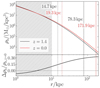 |
Fig. 2. Top panel: Density profile of the highest-mass DM halo of the Sparkler galaxy as predicted by the models by Correa et al. (2015). Black lines indicate the z = 0 profile while red lines the z = 1.378 one. The dotted lines mark r−2, the dashed lines mark r200. The grey shaded area marks the region between 1 and 10 kpc, that is the interval under study. Bottom panel: Difference between the halo density profile at z = 0 and at z = 1.378 normalised to the density profile at z = 0. |
We conclude that the DM density profile of a Sparkler-like galaxy does not substantially change from z ≈ 1.4 to z = 0, at least in the regions of interest for the present work. Therefore, for our purposes, we modelled the halo as an isolated stationary system, neglecting its cosmological evolution and accretion history, by assuming that the galaxy did not undergo any major merger in this interval of time. Finally, we computed the predicted stellar mass of the Sparkler galaxy at z = 0, using the corresponding UNIVERSEMACHINE halo-to-stellar mass relation, finding M*(z = 0) = 8.79 × 10⁹ M⊙, in agreement with the prediction by Adamo et al. (2023) using results from the EAGLE simulation (Crain et al. 2015; Schaye et al. 2015). In Table 4 we list the parameters of the halo of the Sparkler galaxy at z = 1.378 and z = 0, together with the Sparkler stellar mass. For completeness, we include also the parameters of the low-mass halo, obtained from the lowest bound of the estimate of the Sparkler stellar mass.
4. Dynamical friction simulations with single-particle clumps
In this section, we study the effects of dynamical friction on the system of clumps orbiting around the Sparkler galaxy. We first computed the dynamical friction timescale of the clumps in the Sparkler system, in order to assess if this process is expected to play a major role in the dynamical evolution of the clumps. The dynamical friction timescale for a clump with mass Mcl, in a circular orbit at a distance r from the centre of a spherical halo can be estimated as (Binney & Tremaine 2008, Eq. 8.13)
 (12)
(12)
where lnΛ is the Coulomb logarithm, Mh(r) is the mass of the host system within the radius r and tcross = r/vc is the crossing time, with vc = [G Mh(r)/r]1/2 the circular velocity at r. Throughout this work, we assume lnΛ = 10.
In Fig. 3, we show the dynamical friction timescales for a halo defined as in Sect. 3 and for clumps with a mass of 106, 107, and 108 M⊙ and at distances between 1 and 10 kpc. The resulting timescales span a wide range of values, between 0.01 and 100 Gyr. The timescale is comparable to or shorter than the look-back time to z ≈ 1.4 (about 9.23 Gyr) for relevant combinations of distances and masses. Therefore, numerical simulations are needed to quantitatively address the question of whether the clumps sink to the centre of the galaxy by z = 0.
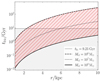 |
Fig. 3. Dynamical-friction timescales for clumps of mass 106, 107, and 108 M⊙ (dashed, dotted and solid lines, respectively) as a function of the distance from the centre of the halo. The red-dashed area covers the range of dynamical friction timescales relative to the interval of clump masses and distances of interest. The grey horizontal line corresponds to the look-back time at z ≈ 1.4 tlb = 9.23 Gyr, that divides the plot between the region in which the dynamical friction is most likely inefficient (tfric > 9.23 Gyr) and efficient (tfric < 9.23 Gyr). The latter is marked by the grey area. |
4.1. Host galaxy model in the simulations
In the simulations presented in this section, we modelled the clumps as single particles, with the Sparkler-like halo set according to the parameters derived in Sect. 3 and listed in Table 4. The halo is made of 107 particles of mass 5.43 × 10⁴ M⊙ each. Modelling the halo by means of DM particles allowed us to directly include the effects of dynamical friction in the simulation thanks to their mutual interaction with the particles representing the clumps.
Throughout our work, we modelled the total mass of the Sparkler system as equal to the aforementioned DM halo mass, unless otherwise stated. The NFW density profile is characterised by a central cusp, such that ρNFW(r ≪ r−2)∝r−1. A central cusp is consistent with the profiles of the total mass (thus including both baryonic and DM components), computed from rotation curves in disc galaxies (such as the SPARC sample, Lelli et al. 2016, with central density logarithmic slope between −1 and −0.5). Therefore, we can assume that the NFW profile is a good representation of the total mass density distribution of a Sparkler-like system.
We defined the initial conditions of the halo following the prescription described in Springel et al. (2005a). By fixing M200 and c200 of the desired NFW potential, the prescription by Springel et al. (2005a) determines the Hernquist (1990) model that most closely resembles the original NFW model in the innermost regions, yet having a finite and converging total mass equal to M200. The Hernquist density profile is
 (13)
(13)
where Mtot is the total mass and a is the scale radius. In our case, Mtot = M200(z = 0), with scale radius a = 32.3 kpc and consequent r200 = 151 kpc. The softening of the gravitational force field was realised adopting a Plummer kernel (Aarseth 1963) with scale-length 150 pc (one third of the average inter-particle distance inside the half-mass radius).
4.2. Simulations of single clumps in circular orbits
As a preliminary numerical exploration, we ran a set of 20 simulations in which one clump, initially on a circular orbit, is followed for 9.23 Gyr in the Sparkler-like halo defined in Sect. 4.1. The initial distance from the centre of the host ranges from 2 to 6 kpc – the range of clump observed distances in the Sparkler galaxy. The explored masses range between 1 × 10⁶ M⊙ and 6 × 10⁷ M⊙, consistent with the observed mass range.
The left panel of Fig. 4 shows the migration of clumps from the initial to the final position, after 9.23 Gyr, for given mass. Clumps with total mass log(M*/M⊙)≤6.3 never reach the centre of the system, even when starting at a distance of 2 kpc. Clumps with higher masses are more effectively brought to the centre of the system: for masses higher than about 3 × 10⁷ M⊙, dynamical friction is extremely efficient across the whole range of initial orbital radii and the clumps reach the centre even when starting at 6 kpc. These results strongly suggest that, if the clumps had a DM halo, and therefore a dynamical mass significantly higher than the stellar mass, it would be very unlikely to observe them in the local Universe, because they would quickly sink to the centre of the system.
 |
Fig. 4. Left panel: Evolution over 9.23 Gyr of the distances from the centre of the point-mass clumps orbiting in a Sparkler-like potential with circular orbit initial conditions. On the x-axis, the mass of the clump is reported, and the black arrows point from the initial to the final distance. The final distance is computed as the average distance from the centre of the system, within the last 5% of the simulated time. The masses larger than the vertical dotted grey line are also larger than the observed stellar masses of the Sparkler clumps. We classify as survived the clumps with final distance out of the shaded area. Right panel: Colour map of the final distance of the clumps as a function of their initial distance (y-axis) and dynamical mass (x-axis), obtained by interpolating the simulations shown in the left panel. The colour bar traces the final distance and goes from 1 kpc (or less) to 6 kpc (the largest simulated initial distance). The contours mark the combinations of initial distance and mass that result in specific values of final distance (from 1 to 5 kpc). The green data points are the extraplanar Sparkler clumps (Claeyssens et al. 2023; Forbes & Romanowsky 2023). For each clump three distances are computed, de-projecting the observed distances depending on the three spatial configurations studied in Sect. 2.4 (face-on disc, edge-on disc, and spherical), as described in Sect. 4.2. The symbols (squares and crosses) indicate the median of the three possible distances, with the error-bars corresponding to the minimum and maximum distance. We used squares for the clumps that survive, while we used crosses for the clumps for which the inferred final distance is smaller than 1 kpc. |
To generalise the results of these simulations to any pair of M*−initial radius in the relevant range, we interpolated the map of the left panel of Fig. 4 using a smooth bivariate spline4. The right panel of Fig. 4 shows the map of the final distance (described by the colour scale) as a function of the initial distance and the mass of the clump. Under these hypotheses, the Sparkler clumps (assumed to contain no DM) are shown in the right panel of Fig. 4. For each clump we computed three estimates of the intrinsic distance, taking into account the possible projection effects of each of the three spatial configurations analysed in Sect. 2.4. In the face-on disc scenario, the observed distance of each clump coincides with the intrinsic one by construction, and therefore no corrections are needed. In the edge-on disc and in the spherical configurations, the de-projected position of the ith clumps is computed as  , where
  is the median of its line-of-sight probability distribution plos, i(|z|). In the edge-on disc configuration, plos, i(z) = pexp[(Robs, i2 + z2)1/2 ; Re], where pexp is the edge-on disc exponential distribution, with effective radius Re (listed in the first row of the third column in Table 3), and Robs, i is the observed position of the ith clump. In the spherical configuration, plos,i(z) = pSersic3D[(Robs, i2 + z2)1/2 ; Re, n], with pSersic3D from Eq. (7), with effective radius Re and Sérsic index n (listed in the first row of the fourth column in Table 3).
As one can notice, seven clumps out of ten fall within 1 kpc from the centre. This experiment hints that dynamical friction is able to drastically change the distribution of the clumps surrounding the Sparkler galaxy. If the clumps do not possess a DM halo, the outermost ones (at 3 − 5 kpc) are poorly affected by dynamical friction, while in the innermost regions only the low-mass ones (less massive than about 5 × 10⁶ M⊙) do not sink to the centre of the system.
4.3. Simulations of Sparkler-like clump system
In this section, in order to assess the effects of dynamical evolution on the Sparkler clumps we ran a series of simulations that explored three Sparkler-like spatial configurations – face-on disc, edge-on disc, or spherical – as defined in Sect. 2.4. Each simulation included 10 clumps with initial masses sampling the distribution discussed in Sect. 2.2. For each spatial configuration we ran 15 simulations, in order to obtain statistically relevant results. The NFW halo, representing the total mass density distribution of the Sparkler galaxy, was built according to the procedure described in Sect. 4.1.
For each simulation, the clump masses were extracted within 3σ of the best-fitting Gaussian distribution (see Table 2). For the initialisation of positions and velocities in the disc configurations (either face-on or edge-on), we used the following steps:
-
Initial distance: extracted from the spatial distribution corresponding to the configuration under study. In particular, the initial distances were imposed to be between 1 and 10 kpc (this interval encloses ≈85% of the total probability).
-
Position angle: randomly extracted under the condition that the clumps were initialised at least at 300 pc (about 10 times the smallest scale radius of the Sparkler clumps, see the discussion in Sect. 2.1) from each other and that the centre of mass of the clump system is consistent with the centre of the halo within the softening length.
-
Velocity: the clumps were initialised on co-planar circular orbits.
For the spherical configuration, the clump initial positions and velocities were extracted from the ergodic distribution function of the system, generated by putting in equilibrium the clump best-fit Sérsic distribution (Eq. (4)) with the Sparkler-like Hernquist gravitational potential, as described in Sect. 4.1. The initial conditions were generated by means of the software code OPOPGADGET5. Since we modelled the evolution of GC-progenitor candidates, that have ages of a few gigayears at z ≈ 1.4 (Mowla et al. 2022; Claeyssens et al. 2023; Adamo et al. 2023), we can neglect mass losses by stellar evolution and keep the mass of the clump-particles constant (Calura et al. 2014).
To illustrate the differences among the three spatial configurations, we present three spatial distributions of ten clumps for each configuration in Figure 5. It is evident that the clumps in the face-on and edge-on disc configurations are co-planar, while in the spherical configuration, they do not occupy the same orbital plane.
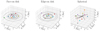 |
Fig. 5. Initial spatial distribution of the ten clumps in representative simulations of the three different spatial configurations described in Sect. 2.4. The initial positions of the clumps are determined as described in Sect. 4.3. From left to right: Face-on disc, Edge-on disc, and Spherical configurations. Each clump is displayed as a coloured dot. In the first two panels, we plot in grey the trajectory of the circular orbit at which each clump is initialised. This also makes apparent that the orbits of the clumps are co-planar in these two configurations. In the right panel, for each clump we plot the projected distance on the x − y plane as the black solid line, and the z coordinate of the clump as the red dotted line, to show that the clumps are not co-planar. |
4.4. Results
We present here the outcomes of the simulations described in Sect. 4.3. In the following, we call the survived clumps all the clumps with a final distance larger than 1 kpc. We computed the final distance as the average distance in the last 5% of the simulation, that is ≈500 Myr, about 25 times the crossing time at 1 kpc. We chose to evaluate the final average distance since clumps on elliptical orbits may have peri-centre distances below our threshold, though they spend most of their time beyond this critical value. We chose this threshold firstly because the focus of this work is on testing the hypothesis that the Sparkler extraplanar clumps are progenitors of local halo or disc GCs, and therefore distances smaller than 1 kpc would be incompatible with such a scenario. Furthermore, the dynamical evolution of the clumps in the central regions depends on a number of factors, such as the central density profile of the DM halo and the presence of substructures and of a proto-bulge, whose modelling goes beyond the scope of this work.
4.4.1. Face-on disc configuration
We first focus on the results obtained for the simulations of the face-on configuration. The top panel in Fig. 6 shows the histogram of the fraction of survived clumps considering the 30 simulations. The median value is  . Interestingly, in all the runs there is at least one survived clump. These results suggest that the Sparkler galaxy is expected to retain 3 − 4 clumps in the outskirts, while the rest of them most likely falls into its centre.
 |
Fig. 6. Fraction of survived clumps of each of the 30 simulations run in the face-on (top panel, in red), edge-on (middle panel, in green) and spherical (bottom panel, in blue) configurations. A clump is flagged as survived if its distance from the centre of the halo at the end of the simulation is larger than 1 kpc. The vertical solid line and the shaded area show the median fraction of survived clumps |

The top panel of Fig. 7 shows the comparison between the initial mass distribution and the mass distribution of survived clumps. The survived distribution gets slightly narrower and peaks at smaller masses than the initial one. Indeed, the mean mass of the survived clumps is  , ≈0.1 dex smaller than the initial one. Even though a non-negligible fraction of ∼107 M⊙ clumps is predicted to survive, the survived clumps are preferentially the low mass ones.
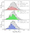 |
Fig. 7. Fraction of initial clumps and survived clumps per mass-bin, shown as grey histograms and coloured histograms (red for the face-on configuration, green for the edge-on configuration and blue for the spherical configuration), respectively. We show the face-on configuration in the top panel, the edge-on configuration in the middle panel, the spherical configuration in the bottom panel. The histograms are built binning all the clumps (either initial or survived) of the 30 simulations, normalised to the initial total number of clumps (ten for each simulation, therefore 300). The black and coloured lines are the best-fitting Gaussian distributions, of which we report the mean in the legend. |
Finally, in the top panel of Fig. 8 we show the clump initial number density profiles (black triangles), projected along the z−axis, compared to the profiles of the survivors at the end of the simulations (red squares). We fitted the latter again with an exponential profile (shown as the red solid line), that still describes remarkably well the distance distribution of the survived clumps. In particular, the best-fitting scale radius is  kpc, larger than the initial value of
  kpc (shown as the dark grey solid line), testifying how most of the lost clumps were in the innermost regions of the system. Indeed, the profile of the survivors is flatter than the initial one.
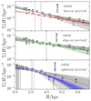 |
Fig. 8. Surface number density profiles of the clumps in the face-on (top panel), edge-on (middle panel), and spherical configuration (bottom panel). In each panel, the dark grey line is the initial distribution, with the grey shaded areas covering the 1σ and 2σ intervals, built adopting the corresponding function described in Sect. 2.4 with the best-fit parameters listed in the first row of Table 3. We projected all the profiles along the z axis. The triangles show the profiles of the initial clump positions in the x − y plane, computed stacking together the 10 clumps in all the 30 runs. The coloured hexagons show the surface number density profiles at the end of the simulations, obtained stacking together all the survived clumps. The corresponding coloured solid line is the best-fit profile to the final projected distances of the survived clumps, obtained as described in Sect. 4.4. We normalised all the profiles to the total number of initial clumps, so the integral of the initial profiles is equal to 1, and the integral of the survived profiles is equal to the average surviving fraction (distributions shown in Fig. 6). |
4.4.2. Edge-on disc configuration
In this configuration, the initial intrinsic distance distribution has a larger scale radius Re than in the face-on disc (see Table 3). As a consequence, the clumps are initialised further from the centre and are less affected by dynamical friction. This difference results in a larger survived fraction (middle panel of Fig. 6), with a median value of  . Therefore, on average, 5 − 6 clumps out of 10 survive down to z = 0. As displayed in the middle panel of Fig. 7, the survived mass distribution is consistent with the face-on one, with a mean stellar mass
  .
.
For what regards the evolution of the spatial distribution, the middle panel of Fig. 8 shows the clump initial number density profile, projected along the z-axis, and the profile of the survived clumps at the end of the simulations. The survived distribution is fitted to an exponential profile following the same method described in Sect. 2.4 and shown as the green solid line, to be compared with the initial profile. The final scale radius of the survived clumps is  kpc, indistinguishable from the initial one (
 ).
).
4.4.3. Spherical configuration
When the configuration is spherical, the fraction of survived clumps (bottom panel in Fig. 6) is  , consistent with the one obtained in the face-on disc case (top panel of Fig. 6). However, the final mass distribution peaks at smaller masses than in both disc configurations, with a mean survived mass
  (bottom panel in Fig. 7). The projected number density profile of the survived clumps remains consistent with the initial one, as shown in the bottom panel of Fig. 8, similarly to what we have found for the edge-on disc configuration. In order to quantitatively compare with the initial distribution (see the solid curves in bottom panel of Fig. 8), we fitted the final distances of survived fraction of clusters to a de-projected Sérsic profile (Eq. (7)), following the same procedure described in Sect. 2.4. The values of the fit parameters (the scale radius and the Sérsic index) are reported in the third column of Table 3 and are consistent with the initial parameters within 1σ.
5. Tidal stripping simulations
In this section, we study the mass evolution of the Sparkler clumps under the effects of the tidal stripping exerted by the gravitational potential of the host system. Assuming that the satellite (a clump in our case) is on a circular orbit around the host system (Sparkler) and that both systems are characterised by a spherical mass distribution, the effects of tidal stripping can be evaluated approximately by computing the tidal radius rtidal. The tidal radius divides the regions in which the satellite mass is highly affected by the host gravitational force (beyond rtidal) from that in which the self-gravity of the satellite is strong enough to retain it (within rtidal). It is defined as the distance from the centre of the satellite at which
 (14)
(14)
where  and
and  are the mean halo and clump densities within r and rtidal, respectively, and r is the distance between the centre of the system and the centre of the clump (see Binney & Tremaine 2008, their Eq. 8.92). We defined the halo density as in Eq. (10), whereas for the clump density we opted for a Plummer density profile (Plummer 1911)
 (15)
(15)
where M* is the total stellar mass and rs is the scale radius. For a Plummer density profile, the projected half-mass radius is Reff = rs.
We computed the fraction of clump mass enclosed within rtidal for clumps of different mass and for distances ranging between 1 and 10 kpc. The results are shown in Fig. 9. For each clump mass, we compute Reff from the size-mass relation (Eq. (1)). The mass within rtidal is always larger than the 86% of the initial total mass. We note that this study is representative only of the sub-sample of seven resolved extraplanar clumps in the Sparkler system. Considering that the upper limits of Reff of the unresolved clumps are 11 − 12 pc, we conclude that they are more compact than the resolved ones. Therefore, they tend to retain more mass than the resolved ones at a given mass. Even though these results are just an approximate prediction, they suggest that the mass loss due to tidal stripping is expected to have minor effects on our predictions about the effects of dynamical friction shown in Sect. 4.4. However, the mass distribution of the clumps can change between z ≈ 1.4 and z = 0 due to mass loss, especially at the low-mass end, and therefore it is useful to model tidal stripping by means of numerical simulations. In the following sections, we describe the simulations that we performed to better study the effects of this process and to test different shapes of the host.
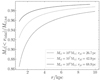 |
Fig. 9. Fraction of the clump mass enclosed within the tidal radius defined as in Eq. (14). The masses of the clumps are 106, 107, and 108 M⊙ (dashed, dotted and solid lines, respectively). The effective radius of the clumps is given by Eq. (1). Tidal radii are computed for distances between 1 and 10 kpc. |
5.1. Tidal stripping in a spherical host
In these experiments, we included the Sparkler total mass as an external potential (i.e. a static potential), while the clumps are resolved. In order to be directly comparable to the mass profile defined in Sect. 4.1, we modelled the external potential as a Hernquist model with the same parameters listed in Sect. 3 and obtained following the procedure described in Springel et al. (2005a).
We modelled the clumps as Plummer spheres (Eq. (15)). Even though the density profile of local GCs is typically well described by the King model (King 1966), we opted for a profile that is still characterised by an inner core, but drops down less steeply in the outskirts. This choice is motivated by the fact that the progenitors of local GCs do not necessarily already possess the final density profile, especially considering that, in the specific case of the Sparkler clumps, both masses and sizes are different from those observed in local GCs. Nonetheless, we verified a posteriori that the clump density becomes comparable to the King profile within ≈500 Myr, since it gets truncated by the galactic tidal field. At a fixed mass M*, the Plummer scale radius rs is given by the size-mass relation (Sect. 2.1). We tested stellar masses between log(M*/M⊙) = 6 and log(M*/M⊙) = 7.8 in steps of 0.3 dex. The clumps are always made of 105 particles with mass M*/105, therefore ranging from 10 M⊙ to 630 M⊙. The softening length is 0.6 pc, about one third of the average inter-particle distance within the clump half-mass radius (≈1.7rs). With this setup, any collisional effect is neglected. Indeed the 2-body relaxation time of these clumps, computed as trelax = 0.1(N/lnN) tcross at the half-mass radius, is in the range between 16 − 33 Gyr (for log(M/M⊙) = 6) and 360 − 720 Gyr (for log(M/M⊙) = 7.8), assuming that the stars have masses in the range 0.5 − 1 M⊙. We initialised the clumps on circular orbits at 1 kpc from the centre of the halo.
In the top panel of Fig. 10, we show the mass retained by the clump relative to the initial one, computed within 4 initial scale radii, as a function of time. The fraction of retained final mass is lower for low-mass clumps than high-mass clumps. However, even for log(M*/M⊙) = 6, less than ≈15% of the initial mass is lost. These results are consistent with the predictions shown in Fig. 9 and confirm that, under the assumption of circular orbit in the considered spherical system, the mass loss due to tidal stripping is negligible.
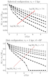 |
Fig. 10. Top panel: Retained mass (relative to the initial one) as a function of time for clumps of different masses in circular orbits at 1 kpc from the centre of the system. The residual mass is computed within 4rs, where rs is the initial Plummer scale radius. In this case, the clumps orbit in a Sparkler-like spherical potential representing the total mass, defined in Sect. 4.1. Masses go from log(M*/M⊙) = 6 to log(M*/M⊙) = 7.8 with a step of 0.3 dex (the arrow points from the smallest to the highest mass). Bottom panel: Same as the left panel but for clumps in quasi-circular orbit at 1 kpc from the centre of the system including a stellar disc component (modelled as in Sect. 5.2). The clump orbital plane is inclined of 30 degrees with respect to the plane of the disc. |
In Appendix B, we also explored the case of clumps on eccentric orbits, starting at larger distances (3 − 4 kpc) and reaching the final distance of ≈1 kpc under the effects of the dynamical friction deceleration, modelled with the Chandrasekhar formula (Chandrasekhar 1943; Binney & Tremaine 2008). However, we obtain that the lost mass is higher than for the circular orbit considered only for clumps in pronounced radial orbits, but only by a factor 2, still insufficient to remove enough mass from the Sparkler clumps in order to reach GC-like masses.
5.2. Tidal stripping in presence of a stellar disc
In Sect. 5.1, we analysed the tidal effects modelling Sparkler as a spherical system. Here, we present the results of a series of simulations of resolved clumps exploring the case in which the stellar component of the host is a disc. This is consistent with the fact that Sparkler is a star-forming galaxy (Mowla et al. 2022). We included a spherical DM halo as an external Hernquist potential similarly to what has been done in Sect. 5.1.
The gravitational field gradient experienced by the clumps as they cross the disc results in the so-called tidal shocks, that can cause the clumps to lose significantly more mass than in the case of spherical symmetry or when the clumps are co-planar with the disc (Gnedin & Ostriker 1997; Kruijssen & Mieske 2009; Lamers & Gieles 2006; Elmegreen & Hunter 2010; Elmegreen 2010; Webb et al. 2014; Kruijssen 2015; Miholics et al. 2017; Pfeffer et al. 2018; Li & Gnedin 2019; Reina-Campos et al. 2022). Aiming at maximising the tidal effects of the disc, for the whole simulation we fixed the disc properties at those that it is predicted to possess at z = 0, after accreting mass for almost 10 Gyr. We determined the disc mass (8.79 × 10⁹ M⊙) as described in Sect. 3, using the halo-to-stellar mass relation at z = 0 from the UNIVERSEMACHINE. The effective radius is Reff = 4.65 kpc, determined from the galaxy mass-size relations by van der Wel et al. (2014), and the disc scale height is hz = 0.25 kpc, in accordance with recent studies of disc galaxies of similar mass and redshift (Bershady et al. 2010; Bacchini et al. 2019, 2024; Ranaivoharimina et al. 2024). We modelled the disc mass density profile with a double exponential profile (Freeman 1970; Binney & Tremaine 2008)
 (16)
(16)
where ρ0 is the central density and Rd is the scale radius. The scale radius Rd = 2.77 kpc is computed from the effective radius Reff following Eq. (13) in Lima Neto et al. (1999), for which we fix the Sérsic index to 1. We modelled the exponential disc as a sum of three Miyamoto-Nagai (MN) disks (Miyamoto & Nagai 1975) of suitable parameters, determined following the prescriptions and correlations by Smith et al. (2015). This choice allowed us to compute the gravitational acceleration of the disc analytically, as the sum of those of the three MN disks. Each MN disc is defined by three parameters (following Eq. (6) in Smith et al. 2015), which we list in Table 5: the total mass Md, the scale radius a and the scale height b. We point out that the disc MN2 (third row in Table 5) has a negative mass, but the sum of the three MN disks results in a density profile that is always positive.
Parameters of the Sparkler-like exponential disc (first row) and of the three MN disks (second, third, and fourth rows) that, summed together, better approximate the potential of the original exponential disc (see Smith et al. 2015).
Similarly to what has been done in the previous section, we varied the mass of the clumps from log(M*/M⊙) = 6 to log(M*/M⊙) = 7.8 (with steps of 0.3 dex) and determined the size from the Sparkler size-mass relation (Eq. (1)). The initial conditions of the centre of mass of the clumps were always set in the same way. The initial position was (x0, y0, z0) = (r0 cos ϑ, 0, r0 sin ϑ), with ϑ = π/6. Therefore we initialised the clump at a distance of r0 = 1 kpc, with the initial position vector inclined by 30 degrees with respect to the plane of the disc (coinciding with the x − y plane). The initial velocity was (vx, 0, vy, 0, vz, 0) = (0, vc, 0, 0), where vc, 0 is the speed of an object in circular orbit at R = r0 and z = 0 co-planar to the disc. Therefore, the initial speed was given by the relation vc, 02 = G Mhalo(r0)/r0 + r0[dΦdisk/dR](r0, 0), where Φdisk(R, z) is the disc potential.
We tested many values of ϑ finding that, for ϑ > π/6, the orbits are such that the distance of the clump from the centre of the system displays significant variations, experiencing a number of close peri-centric passages, yet showing similar effects in terms of mass loss. Therefore we opted for ϑ = π/6, for which the clump keeps an almost-constant distance from the centre of the system, without losing the effects of tidal shocks. We fixed the initial distance at r0 = 1 kpc in order to maximise the tidal effects within the interval of observed clump distances. In Fig. 11 we show the first 0.51 Gyr of the orbit, on the x − y and x − z planes, for the case of a clump with M* = 106 M⊙. We note that the orbit is limited to a finite volume, represented by a thick ring in the x − y plane and by a box in the x − z plane, even though the distance of the clump from the centre of the system remains close to 1 kpc, with variations as large as 10%. Furthermore, the snapshot at 0.51 Gyr already shows the effects of the tidal shocks, with long tails of stellar particles departing from the main body of the clump. Finally, we note that, since in these simulations we included the Sparkler potential as an external potential, the clump is unaffected by dynamical friction, so the clump does not inspiral.
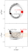 |
Fig. 11. Comparison between the initial conditions and the snapshot at 0.51 Gyr for the tidal-shock simulation described in Sect. 5.2 in the case of mass M* = 106 M⊙. The top and bottom panels show the projections on the x − y and x − z planes, respectively. The clump stellar particles are shown as red and black dots for the snapshots at t = 0 Gyr and t = 0.51 Gyr, respectively. The centres of clumps at t = 0 Gyr and t = 0.51 Gyr are shown as a black and red star, respectively, with an horizontal line of length 4 rs, i, where rs, i is the initial Plummer scale radius. The grey dashed curves represent the trajectory of the clump. The orange curves trace iso-density contours of the Sparkler disc external potential. The centre of the system is marked by a black cross. |
We show the resulting retained clump mass as a function of time in the bottom panel of Fig. 10, which demonstrates how the tidal shocks strongly change the results with respect to the spherical configuration shown in the top panel. A clump of log(M*/M⊙) = 7.8 retains about 70 − 75% of the initial mass (with respect to > 90% in the absence of a disc), while a clump with mass log(M*/M⊙) = 6 gets completely disrupted (without a disc it retains about 90% of its initial mass). Again, we point out that these results are relative to the most extreme cases of tidal shocks, since we considered the highest possible mass for a Sparkler-like disc and the clumps are very close to the central regions. Therefore, not all the clumps as small as 106 M⊙ are disrupted. However, at the same time, even in presence of tidal shocks the massive clumps tend to remain particularly massive if compared with the typical mass of present-day GCs.
6. Discussion
The results presented in Sects. 4 and 5 suggest that the fraction of surviving clumps is ≈40 − 60%. Previous N-body simulations of MW-like (Pfeffer et al. 2018; Reina-Campos et al. 2019; Li & Gnedin 2019) and dwarf (Moreno-Hilario et al. 2024) galaxies find smaller surviving fraction (10 − 30%). This difference, yet not particularly pronounced, may arise from many different factors, such as the different mass of the simulated host system. The simulations presented in Sect. 4 did not include tidal stripping effects, which, on the one hand, may increase the fraction of lost clumps as a consequence of their disruption but, on the other hand, may also halt the sinking caused by dynamical friction. Furthermore, in this work we focused on the clumps located far away from the main body of the galaxy, neglecting those observed within it and therefore closer to the centre of the system and more susceptible to dynamical friction. The fraction of survivors among these clumps would most likely be smaller, decreasing the average fraction of total survivors. Finally, the sample of clumps observed in the Sparkler galaxy is most likely biased towards the high-mass end of the clump mass distribution, even though the sample completeness in lensed images is very difficult to study.
The mass distribution of the survivors changes from the initial one only for the loss of the clumps accreted onto the centre of the system. Tidal stripping from a spherical host system, presented in Sect. 5.1, has a minor effect on shaping the final mass distribution. Therefore, in the scenario in which the Sparkler galaxy is better described by a spherical geometry, our study predicts the presence of very massive surviving clumps, more massive than 107 M⊙ and inconsistent with the observed properties of present-day GCs in a Sparkler-like progenitor (see Baumgardt & Hilker 2018 for the MW; Baumgardt et al. 2013 for the Large Magellanic Cloud; Hunter et al. 2003 for the Small Magellanic Cloud). Such outliers are very uncommon in the local Universe. Some effects not taken into account in our simulations can be additional channels to remove mass from these clumps or completely disrupt them. For example, the presence of DM in the clumps would increase their mass and enhance the dynamical friction efficiency, bringing them to the centre on shorter timescales. Alternatively, if these clumps were accreted by a previous merger or are ejected from the disc by a subsequent one, the orbits of the clumps would tend to be eccentric. The small peri-centric distances of such orbits can favour both dynamical friction and tidal stripping effects, and therefore their fall to the centre of the system or the loss of the stellar mass in excess (Gnedin & Ostriker 1997; Gnedin et al. 1999; Baumgardt & Makino 2003; Webb et al. 2013, 2014; Brockamp et al. 2014). Finally, a number of works (Gieles et al. 2006; Lamers & Gieles 2006; Webb et al. 2019, 2024; Reina-Campos et al. 2022) have shown that the encounters with giant molecular clouds (GMCs) cause a series of tidal shocks able to significantly strip mass from the clumps. However, we note that these works conclude that a high frequency of encounters with GMCs is needed in order to make the tidal shocks effective. Therefore this process is effective if the clumps have formed and orbit inside the stellar disc; on the other hand, if the clumps are located outside the stellar disc and cross it only twice per orbital period (as modelled in Sect. 5.2), then the interactions with the GMCs are not frequent enough and therefore negligible with respect to the tidal shocks exerted by the stellar disc.
6.1. Clump size evolution
The half-mass radii of GCs in the local Universe are typically of a few parsecs (Jordán et al. 2005; Spitler et al. 2006; Baumgardt et al. 2023). Therefore, the size of the Sparkler clumps must evolve to similar to consistent values, down to z = 0, in order to be promising GC progenitors.
By removing the outermost stars of the clumps, tidal stripping reduces the half-mass radius. To quantify this effect, we took the final snapshot of each simulation presented in Sects. 5.1 and 5.2 and fitted the clump to a Plummer sphere (Eq. (15)). The fitting procedure is described in detail in Appendix A and gives us the final total mass M*, f and scale radius rs, f. In Fig. 12, we compare the initial scale radii rs, i with the final ones, both for the tidal stripping in a spherical system, and for tidal shocks of a Sparkler-like disc. Such sizes, even considering the effects of tidal stripping and shocks, remain systematically larger than 20 pc down to z = 0, with the only exception of the clump with mass 106 M⊙ in the tidal shock simulation, which gets completely disrupted. Therefore, the final sizes of these clumps are incompatible with those observed in local GCs.
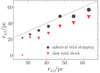 |
Fig. 12. Comparison between the final (rs, f) and initial (rs, i) scale radii of the clumps simulated in Sect. 5 when modelled as a Plummer sphere, as in Eq. (15). The initial scale radii are computed from the size-mass relation of Sect. 2.1. The final scale radii are obtained fitting a Plummer density profile to the final snapshots of the simulations of resolved clumps in a spherically symmetric Sparkler-like system (Sect. 5.1, circles) and of the simulations including the effects of a disc (Sect. 5.2, triangles). The dashed line is the 1 : 1 relation. |
If one assumed that the observed sizes of these objects are overestimated because of the limited angular resolution of JWST, thus not affecting the mass estimate, and that these clumps possess actual GC-like sizes, then the clumps would become even denser, making the tidal stripping negligible. This would imply that the over-massive surviving outliers discussed in the previous section would become even more difficult to strip of their excess mass. Alternatively, if the magnification factors μ of the clumps were underestimated, then their intrinsic properties would be biased towards large values. The intrinsic mass of a lensed object mi is related to the observed and lensed one mo by mi = mo/μ, while the intrinsic length li is related to the observed and lensed one by li = lo/μ1/2. If, for instance, the true magnification factor were underestimated by a factor ≈10, then the clumps would have masses consistent with those of massive local GCs and sizes larger by a factor up to 5. A magnification factor μ ≈ 100 would be consistent with the one of the critical line derived for the Sparkler galaxy by Mahler et al. (2023).
6.2. Combining dynamical friction and tidal shocks
In this section, we combine our dynamical friction and tidal shock results, in order to predict the expected mass distribution of the survived Sparkler clumps at z = 0. For this experiment, we considered the spherical configuration described in Sect. 2.4. In this scenario, the clump orbits are not co-planar to the stellar disc of the Sparkler system, and therefore they undergo a series of tidal shocks in correspondence of the crossings of the galactic disc, as modelled in Sect. 5.2.
The mass losses triggered by the tidal shocks can affect the orbital evolution of the clump (see the bottom panel of Fig. 7) since a lower mass results in a less efficient dynamical friction. In order to quantify these tidal effects, we modelled the relation between the final fraction of mass lost |ΔM*, fin|/M*, in and the initial mass M*, in as
![Mathematical equation: $$ \begin{aligned} \log (|\Delta M_{*,\mathrm{fin} }|/M_{*,\mathrm{ini} })=\mathrm{min} [m\,\log (M_{*,\mathrm{ini} }/{\mathrm{M} _{\odot }}) + q,0], \end{aligned} $$](/articles/aa/full_html/2025/09/aa54669-25/aa54669-25-eq63.gif) (17)
(17)
which we report in the left panel of Fig. 13. We quantified the mass losses as described in Sect. 5.2, as the difference between the initial and final mass within four initial Plummer scale radii. According to this model, there is a minimum mass M*, min below which the clumps are always destroyed. Since our results show that a clump of mass 106 M⊙ is completely disrupted, M*, min must be close to such a value. The best-fitting parameters obtained by means of the non-linear least squares method, implemented in the NUMPY6 function CURVE_FIT, are m = −0.35 ± 0.02 and q = 2.06 ± 0.15, that roughly correspond to M*, min = 8 × 10⁵ M⊙.
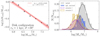 |
Fig. 13. Left panel: Fraction of the clump mass lost after 9.23 Gyr |ΔM*, fin|/M*, ini as a function of the initial mass M*, ini. Here ΔM*, fin = M*, fin(4rs)−M*, ini, where M*, fin(4rs) is the final mass within four initial Plummer scale radii, computed as in Sect. 5.2. The circles are the results from the simulations of resolved clumps described in Sect. 5.2, while the line is the best fit (Eq. 17) and the shaded area is the 1σ interval. Right panel: Distributions of the number of clumps per mass bin, normalised to the total initial number of clumps. The grey and blue histograms are the analogues of those shown in the bottom panel of Fig. 7, and they show the initial and surviving number of clumps, respectively, in the spherical configuration case considering the effects of dynamical friction only. The purple histogram shows the mass distribution of the surviving clumps of scenario 1 (short dynamical-friction timescale; Sect. 5.2), while the golden histogram shows the mass distribution of the surviving clumps of scenario 2 (short tidal-stripping timescale; Sect. 5.2). A Gaussian function is fitted to each histogram and shown with the corresponding colour. |
In order to understand how the final clump mass distribution changes, we consider two different scenarios: 1) the dynamical-friction timescale is shorter than the tidal-stripping one and 2) the tidal-stripping timescale is shorter than the dynamical-friction one. We show the resulting fractions of survived clumps per mass bin in the right panel of Fig. 13 as the purple and golden histograms, respectively, together with the initial distribution in grey and the results from Sect. 4.4.3 in blue. We computed the mass distributions as follows:
-
Scenario 1: starting from the mass distribution of survived clumps discussed in Sect. 4.4.3, shown in the right panel of Fig. 13 with the blue histogram, the final masses are shifted at lower masses because of tidal stripping, according to the model of Eq. (17) (the purple histogram in the right panel in Fig. 13). Low-mass clumps are shifted below 106 M⊙, in a regime that is absent in the initial distribution, while the massive survived clumps do not change significantly their mass;
-
Scenario 2: as a first step, we shift the initial mass distribution according to the model of Eq. (17). Then, we computed the fraction of survived clumps per mass bin as the ratio between the number of survived clumps in the spherical dynamical friction-only scenario and the number of total clumps (blue and grey histogram in the right plot of Fig. 13, respectively). We show the final result as the golden histogram: similarly to scenario 1, a good fraction of clumps is shifted to masses comparable with those of massive local GCs, yet retaining ≈16% of clumps with masses above the mass of ω Centauri (5 × 10⁶ M⊙). Furthermore, in this scenario the fraction of survived clumps increases from 0.42 of the spherical dynamical friction-only case to 0.60.
If we compare scenario 1 and scenario 2, we note that the low-mass end is very similar, while the high-mass end in scenario 2 reaches higher clump masses than in scenario 1. This is a consequence of the fact that the tidal shocks reduce the mass of very massive clumps, affecting the efficiency of the dynamical friction. Nonetheless, the two final mass distributions are very similar: this is a remarkable result since it implies that in the Sparkler system the relative efficiency of dynamical friction and tidal shock mainly affects the number of survivors, but not their mass distribution. The mean masses for scenario 1 and scenario 2 are indeed  and
and  , respectively. Both values are smaller than the one in absence of tidal effects, but consistent within 1σ. The fraction of survived over-massive clusters (M* > 5 × 10⁶ M⊙, the mass of ω Centauri) is between 0.07 and 0.16 (scenario 1 and 2, respectively).
However, we note once again that our assumptions aimed at maximising the tidal effects and therefore the shift applied to the distribution of survival clumps in the spherical configuration. This would imply an over-estimate of the fraction of low-mass clumps and an under-estimate of the fraction of high-mass clumps.
6.3. The fate of the accreted clumps
The accretion of massive clumps, that are more frequent at high redshift and more affected by dynamical friction, has been proposed as an efficient channel for the formation and mass growth of galactic bulges (Scannapieco & Tissera 2003; Hopkins et al. 2010). Such a scenario has been supported in the past couple of decades by the observation of massive GCs, namely Terzan 5 and Liller 1, within 1 kpc from the centre of the MW. These GCs, also called bulge fossil fragments (BFFs), have present-day stellar masses of a few 106 M⊙ (Lanzoni et al. 2010; Saracino et al. 2015; Baumgardt et al. 2023) and are supposed to be among the few surviving stellar clusters that contributed to the Galactic bulge build-up. Recent studies based on their metallicity and star formation history have concluded that the initial stellar mass of the progenitors of these BFFs ranges from 4 × 10⁷ M⊙ (Romano et al. 2023; Crociati et al. 2024) up to 109 M⊙ (Ferraro et al. 2021). The masses of the clumps accreted by the centre of the Sparkler galaxy (Sect. 4) are consistent with the values found by Romano et al. (2023) for the progenitors of the BFFs, favouring a scenario in which a fraction of the clumps observed around the Sparkler galaxy are BFF progenitors. We point out that the half-mass radii of Terzan 5 and Liller 1 are 4.03 and 2.42 pc, respectively, a factor ∼10 smaller than the sizes of the Sparkler resolved clumps, as discussed in Sect. 6.1. However, we remind the presence of three unresolved clumps among those of our sample. In particular, C4 and C9 have masses larger than 107 M⊙ and upper limits on their effective radii of 11 − 12 pc (Table 1), making them promising BFF progenitors also in terms of size.
Another possible evolutionary path of the massive clumps of Sparkler is the one leading to the formation of a nuclear star cluster (NSC; see e.g. Neumayer et al. 2020). The NSCs are located by definition at the dynamical centre of the host galaxy and are usually detected from the light excess above the extrapolation of the host galaxy’s surface brightness profile into its innermost regions (≲102 pc). NSCs are found in both early- and late-type galaxies and are usually the brightest clusters of their hosts, possibly as a consequence of the merging of the clumps and GCs fallen into the centre of the system, dragged by dynamical friction (Tremaine et al. 1975; Capuzzo-Dolcetta 1993; Oh & Lin 2000; Agarwal & Milosavljević 2011; Neumayer et al. 2011). Their effective radii are usually of a few parsecs, but a non-negligible fraction of NSCs with sizes larger than 10 pc exists (Georgiev et al. 2016) and would be compatible with those of the Sparkler clumps. Their masses are typically higher than those of GCs and consistent with those of the Sparkler clumps, peaking at ∼ 106−7 M⊙ and reaching also values as large as ∼ 108−9 M⊙ (Georgiev et al. 2016).
Finally, we note that the simulations presented in this work are not capable of capturing the complex processes that a clump undergoes in the centre of the Sparkler galaxy. Therefore at the moment, we are unable to quantify the fraction of accreted clumps that are completely disrupted, survive as BFFs, or sink and merge to the very centre of Sparkler forming a NSC.
7. Conclusions
In this work we studied the dynamical evolution of the stellar clump system observed in the Sparkler gravitationally lensed galaxy at z ≈ 1.4. We focused our study on the clumps observed far away from the galactic stellar component, among which recent JWST photometric observations have hinted at the presence of candidate progenitors of the GCs observed in the local Universe (Mowla et al. 2022; Claeyssens et al. 2023; Adamo et al. 2023). These objects, consistent with GCs in terms of formation redshift and metallicity, possess very large masses (log(M*/M⊙) = 6.3 − 7.4) and sizes (half-mass radii Reff = 30 − 52 pc) and are located at projected distances from the centre of the galaxy of 2 − 5 kpc. Their dynamical evolution from z ≈ 1.4 to z = 0 (about 9.23 Gyr) can affect not only their position in the galactic system but also their final mass and size.
We first focused on their evolution by taking into account the effect of the dynamical friction exerted by the Sparkler system, modelled as a spherical system. Since little is known about the morphology of the galaxy and of the clump system, we studied three possible configurations: a face-on disc, an edge-on disc, and a spherical geometry. The disc configurations (Sects. 4.4.1 and 4.4.2) are relevant in the context of GC formation. According to previous works, GCs may form in the galactic discs in an epoch of bursty star formation (favoured in the star-forming sites of disc galaxies) and then be ejected far away from the galactic plane by subsequent major mergers (Hopkins et al. 2009; Kruijssen et al. 2012; Kruijssen 2015). In the first two configurations, we initialised the clumps on circular orbits co-planar to each other, while in the third, we assumed the clump system to be spherically symmetric and isotropic. For each scenario, we performed multiple simulations of Sparkler-like clump systems, computing the number of survived clumps (that ended the simulation at a distance larger than 1 kpc from the centre of the system) and the mass and distance distributions. The main results of these simulations can be summarised as follows:
-
On average, about four clumps per simulation survive, depending on the scenario, while the others are accreted onto the centre of the system.
-
The distance distribution remains essentially unchanged, with the only exception being the face-on disc case in which the final distance distribution is more extended than the initial one.
-
The final mass distribution slightly shifts to smaller masses, but the peak value
 remains larger than ∼6.7. Therefore, a significant fraction of survived clumps are more massive than a few 106 M⊙, which is unexpected for a galaxy such as Sparkler, that is thought to reach a stellar mass of 109−10 M⊙ at z = 0.
In addition to the aforementioned simulations, we also studied the clump mass loss under the effects of the tidal field of the host galaxy by means of a different simulation setup in which we implemented the Sparkler system as an external gravitational potential and the clumps as resolved Plummer spheres made of 105 particles. We tested both the case in which Sparkler is a spherical system and in which the Sparkler stellar component is an exponential disc. In the presence of a disc, we initialised the clumps at 1 kpc outside the plane of the disc, experiencing strong tidal shocks every time they cross such a plane as a consequence of the large gravitational field gradient. The main outcome of these simulations are as follows:
-
In the spherical case, the fraction of mass lost is smaller than ≈15% at any clump stellar mass.
-
In the presence of the stellar disc, tidal shocks can completely disrupt low-mass clumps, while they have minor effects for very massive clumps.
-
Even when a large fraction of mass is removed, the sizes of the clumps remain between 20 and 50 pc, that is about a factor of ten larger than the sizes typically observed in local GCs.
When combining the aforementioned results of dynamical friction and tidal shock from a disc, we bracketed a realistic behaviour. If we consider first the mass lost by tidal shocks, the diminished mass of the clumps partially halts the effects of dynamical friction. Consequently, the fraction of survivors increases to 60% of the initial sample. On the other hand, if we consider first the evolution of the mass distribution under the effects of dynamical friction, the mass loss caused by the tidal shocks shifts the mass distribution of the survived clumps at smaller values. In both cases, the peak mass is  . Such values are marginally consistent with the high-mass end of the mass distribution of MW GCs (Baumgardt & Hilker 2018), even though we note the strong difference between the sizes of the Sparkler clumps and those of local GCs.
Apart from the possible underestimate of the lensing magnification factor of the clumps, further effects not considered in this work, such as preferentially radial orbits and encounters with giant molecular clouds, may increase the fraction of stripped mass, explaining these outliers. Radial orbits make the clump explore the innermost and densest regions of the system, experiencing a larger tidal field (Gnedin & Ostriker 1997; Gnedin et al. 1999; Baumgardt & Makino 2003; Webb et al. 2013, 2014; Brockamp et al. 2014). Close encounters with dense and massive molecular clouds can trigger a number of tidal shocks (Gieles et al. 2006; Lamers & Gieles 2006; Webb et al. 2019, 2024; Reina-Campos et al. 2022). Alternatively, these objects may possess DM mini-halos that would justify the observed sizes, more consistent with those of dwarf galaxies than GCs (Tolstoy et al. 2009). In such a case, they would sink more efficiently to the centre of the system, owing to their higher mass, explaining the absence of these over-massive outliers at low redshift. On top of that, a major merger occurring between z ≈ 1.4 and z = 0 could strongly affect the spatial distribution and orbital properties of the clumps, possibly ejecting them into the galactic halo (Kruijssen et al. 2012). However, the clump ejection would limit further dynamical process, making it hard to strip the excess mass (Pfeffer et al. 2018; Li & Gnedin 2019). Finally, it is not excluded that the Sparkler galaxy could actually be an uncommon system and have no counterparts in the present-dayUniverse.
Our study shows how the morphology of the Sparkler galaxy and that of its clump system affect the dynamical evolution of the clumps and suggests that most of the observed Sparkler clumps are likely to sink to the centre of the system, rather than being disrupted by tidal stripping. Once they reach the central regions, these clumps can eventually contribute to the formation of the bulge or survive as a compact stellar system similar to those observed in recent studies of the MW bulge or eventually merge, forming a nuclear star cluster. The survived clumps tend to have masses and sizes larger than the expected values observed in the GCs of the MW. Future data constraining the kinematics and morphology of the Sparkler galaxy and its clump system will help shed light on the dynamical evolution of candidate proto-GCs by making it possible to build more realistic models of this galaxy.
Acknowledgments
We thank the anonymous referee for their useful comments that helped improve this manuscript. The research activities described in this paper have been co-funded by the European Union – NextGenerationEU within PRIN 2022 project n.20229YBSAN – Globular clusters in cosmological simulations and in lensed fields: from their birth to the present epoch. This research made use of Astropy, a community developed core Python package for Astronomy by the Astropy Collaboration (2018).
References
- Aarseth, S. J. 1963, MNRAS, 126, 223 [NASA ADS] [Google Scholar]
- Adamo, A., Usher, C., Pfeffer, J., & Claeyssens, A. 2023, MNRAS, 525, L6 [NASA ADS] [CrossRef] [Google Scholar]
- Agarwal, M., & Milosavljević, M. 2011, ApJ, 729, 35 [NASA ADS] [CrossRef] [Google Scholar]
- Astropy Collaboration (Price-Whelan, A. M., et al.) 2018, AJ, 156, 123 [Google Scholar]
- Bacchini, C., Fraternali, F., Iorio, G., & Pezzulli, G. 2019, A&A, 622, A64 [NASA ADS] [CrossRef] [EDP Sciences] [Google Scholar]
- Bacchini, C., Nipoti, C., Iorio, G., et al. 2024, A&A, 687, A115 [NASA ADS] [CrossRef] [EDP Sciences] [Google Scholar]
- Bagla, J. S. 2002, J. Astrophys. Astron., 23, 185 [NASA ADS] [CrossRef] [Google Scholar]
- Barnes, J., & Hut, P. 1986, Nat., 324, 446 [Google Scholar]
- Baumgardt, H., & Hilker, M. 2018, MNRAS, 478, 1520 [Google Scholar]
- Baumgardt, H., & Makino, J. 2003, MNRAS, 340, 227 [NASA ADS] [CrossRef] [Google Scholar]
- Baumgardt, H., Parmentier, G., Anders, P., & Grebel, E. K. 2013, MNRAS, 430, 676 [NASA ADS] [CrossRef] [Google Scholar]
- Baumgardt, H., Hénault-Brunet, V., Dickson, N., & Sollima, A. 2023, MNRAS, 521, 3991 [CrossRef] [Google Scholar]
- Behroozi, P., Wechsler, R. H., Hearin, A. P., & Conroy, C. 2019, MNRAS, 488, 3143 [NASA ADS] [CrossRef] [Google Scholar]
- Bekki, K., & Freeman, K. C. 2003, MNRAS, 346, L11 [Google Scholar]
- Bekki, K., & Tsujimoto, T. 2019, ApJ, 886, 121 [NASA ADS] [CrossRef] [Google Scholar]
- Bershady, M. A., Verheijen, M. A. W., Westfall, K. B., et al. 2010, ApJ, 716, 234 [NASA ADS] [CrossRef] [Google Scholar]
- Binney, J., & Tremaine, S. 2008, Galactic Dynamics, Second Edition (Princeton University Press) [Google Scholar]
- Binney, J., & Wong, L. K. 2017, MNRAS, 467, 2446 [NASA ADS] [Google Scholar]
- Brockamp, M., Küpper, A. H. W., Thies, I., Baumgardt, H., & Kroupa, P. 2014, MNRAS, 441, 150 [CrossRef] [Google Scholar]
- Brown, G., & Gnedin, O. Y. 2021, MNRAS, 508, 5935 [NASA ADS] [CrossRef] [Google Scholar]
- Bryan, G. L., & Norman, M. L. 1998, ApJ, 495, 80 [NASA ADS] [CrossRef] [Google Scholar]
- Calura, F., Ciotti, L., & Nipoti, C. 2014, MNRAS, 440, 3341 [NASA ADS] [CrossRef] [Google Scholar]
- Calura, F., D’Ercole, A., Vesperini, E., Vanzella, E., & Sollima, A. 2019, MNRAS, 489, 3269 [Google Scholar]
- Calura, F., Lupi, A., Rosdahl, J., et al. 2022, MNRAS, 516, 5914 [Google Scholar]
- Calura, F., Pascale, R., Agertz, O., et al. 2025, A&A, 698, A207 [NASA ADS] [CrossRef] [EDP Sciences] [Google Scholar]
- Capuzzo-Dolcetta, R. 1993, ApJ, 415, 616 [NASA ADS] [CrossRef] [Google Scholar]
- Chandrasekhar, S. 1943, ApJ, 97, 255 [Google Scholar]
- Ciotti, L., & Bertin, G. 1999, A&A, 352, 447 [NASA ADS] [Google Scholar]
- Claeyssens, A., Adamo, A., Richard, J., et al. 2023, MNRAS, 520, 2180 [NASA ADS] [CrossRef] [Google Scholar]
- Claeyssens, A., Adamo, A., Messa, M., et al. 2025, MNRAS, 537, 2535 [Google Scholar]
- Correa, C. A., Wyithe, J. S. B., Schaye, J., & Duffy, A. R. 2015, MNRAS, 452, 1217 [CrossRef] [Google Scholar]
- Crain, R. A., Schaye, J., Bower, R. G., et al. 2015, MNRAS, 450, 1937 [NASA ADS] [CrossRef] [Google Scholar]
- Crociati, C., Cignoni, M., Dalessandro, E., et al. 2024, A&A, 691, A311 [NASA ADS] [CrossRef] [EDP Sciences] [Google Scholar]
- Di Cintio, P., Iorio, G., Calura, F., Nipoti, C., & Cantari, M. 2024, A&A, 690, A61 [NASA ADS] [CrossRef] [EDP Sciences] [Google Scholar]
- Diemer, B. 2018, ApJS, 239, 35 [NASA ADS] [CrossRef] [Google Scholar]
- Dutton, A. A., & Macciò, A. V. 2014, MNRAS, 441, 3359 [Google Scholar]
- Elmegreen, B. G. 2010, ApJ, 712, L184 [Google Scholar]
- Elmegreen, B. G., & Hunter, D. A. 2010, ApJ, 712, 604 [NASA ADS] [CrossRef] [Google Scholar]
- Ferraro, F. R., Pallanca, C., Lanzoni, B., et al. 2021, Nat. Astron., 5, 311 [Google Scholar]
- Forbes, D. A., & Romanowsky, A. J. 2023, MNRAS, 520, L58 [Google Scholar]
- Freeman, K. C. 1970, ApJ, 160, 811 [Google Scholar]
- Georgiev, I. Y., Böker, T., Leigh, N., Lützgendorf, N., & Neumayer, N. 2016, MNRAS, 457, 2122 [Google Scholar]
- Gieles, M., Zwart, S. F. P., Baumgardt, H., et al. 2006, MNRAS, 371, 793 [NASA ADS] [CrossRef] [Google Scholar]
- Gnedin, O. Y., & Ostriker, J. P. 1997, ApJ, 474, 223 [Google Scholar]
- Gnedin, O. Y., Hernquist, L., & Ostriker, J. P. 1999, ApJ, 514, 109 [NASA ADS] [CrossRef] [Google Scholar]
- Hernquist, L. 1990, ApJ, 356, 359 [Google Scholar]
- Hopkins, P. F., Cox, T. J., Younger, J. D., & Hernquist, L. 2009, ApJ, 691, 1168 [NASA ADS] [CrossRef] [Google Scholar]
- Hopkins, P. F., Bundy, K., Croton, D., et al. 2010, ApJ, 715, 202 [Google Scholar]
- Horta, D., Hughes, M. E., Pfeffer, J. L., et al. 2021, MNRAS, 500, 4768 [Google Scholar]
- Hunter, D. A., Elmegreen, B. G., Dupuy, T. J., & Mortonson, M. 2003, AJ, 126, 1836 [NASA ADS] [CrossRef] [Google Scholar]
- Jordán, A., Côté, P., Blakeslee, J. P., et al. 2005, ApJ, 634, 1002 [CrossRef] [Google Scholar]
- King, I. R. 1966, AJ, 71, 64 [Google Scholar]
- Kravtsov, A. V., & Gnedin, O. Y. 2005, ApJ, 623, 650 [Google Scholar]
- Kruijssen, J. M. D. 2015, MNRAS, 454, 1658 [Google Scholar]
- Kruijssen, J. M. D., & Mieske, S. 2009, A&A, 500, 785 [NASA ADS] [CrossRef] [EDP Sciences] [Google Scholar]
- Kruijssen, J. M. D., Pelupessy, F. I., Lamers, H. J. G. L. M., et al. 2012, MNRAS, 421, 1927 [NASA ADS] [CrossRef] [Google Scholar]
- Lamers, H. J. G. L. M., & Gieles, M. 2006, A&A, 455, L17 [NASA ADS] [CrossRef] [EDP Sciences] [Google Scholar]
- Lanzoni, B., Ferraro, F. R., Dalessandro, E., et al. 2010, ApJ, 717, 653 [Google Scholar]
- Lee, Y. W., Joo, J. M., Sohn, Y. J., et al. 1999, Nat., 402, 55 [Google Scholar]
- Lelli, F., McGaugh, S. S., & Schombert, J. M. 2016, AJ, 152, 157 [Google Scholar]
- Li, H., & Gnedin, O. Y. 2019, MNRAS, 486, 4030 [NASA ADS] [CrossRef] [Google Scholar]
- Lima Neto, G. B., Gerbal, D., & Márquez, I. 1999, MNRAS, 309, 481 [Google Scholar]
- Mackey, A. D., & Gilmore, G. F. 2004, MNRAS, 355, 504 [NASA ADS] [CrossRef] [Google Scholar]
- Mahler, G., Jauzac, M., Richard, J., et al. 2023, ApJ, 945, 49 [CrossRef] [Google Scholar]
- Meštrić, U., Vanzella, E., Zanella, A., et al. 2022, MNRAS, 516, 3532 [CrossRef] [Google Scholar]
- Miholics, M., Kruijssen, J. M. D., & Sills, A. 2017, MNRAS, 470, 1421 [Google Scholar]
- Miyamoto, M., & Nagai, R. 1975, PASJ, 27, 533 [NASA ADS] [Google Scholar]
- Moreno-Hilario, E., Martinez-Medina, L. A., Li, H., Souza, S. O., & Pérez-Villegas, A. 2024, MNRAS, 527, 2765 [Google Scholar]
- Mowla, L., Iyer, K. G., Desprez, G., et al. 2022, ApJ, 937, L35 [NASA ADS] [CrossRef] [Google Scholar]
- Navarro, J. F., Frenk, C. S., & White, S. D. M. 1996, ApJ, 462, 563 [Google Scholar]
- Neumayer, N., Walcher, C. J., Andersen, D., et al. 2011, MNRAS, 413, 1875 [NASA ADS] [CrossRef] [Google Scholar]
- Neumayer, N., Seth, A., & Böker, T. 2020, A&ARv, 28, 4 [Google Scholar]
- Oh, K. S., & Lin, D. N. C. 2000, ApJ, 543, 620 [NASA ADS] [CrossRef] [Google Scholar]
- Pallottini, A., Ferrara, A., Gallerani, S., et al. 2022, MNRAS, 513, 5621 [NASA ADS] [Google Scholar]
- Pascale, R., Calura, F., Vesperini, E., et al. 2025, A&A, 699, A31 [NASA ADS] [CrossRef] [EDP Sciences] [Google Scholar]
- Petts, J. A., Read, J. I., & Gualandris, A. 2016, MNRAS, 463, 858 [NASA ADS] [CrossRef] [Google Scholar]
- Pfeffer, J., Kruijssen, J. M. D., Crain, R. A., & Bastian, N. 2018, MNRAS, 475, 4309 [Google Scholar]
- Plummer, H. C. 1911, MNRAS, 71, 460 [Google Scholar]
- Pontoppidan, K. M., Barrientes, J., Blome, C., et al. 2022, ApJ, 936, L14 [NASA ADS] [CrossRef] [Google Scholar]
- Posti, L., & Helmi, A. 2019, A&A, 621, A56 [NASA ADS] [CrossRef] [EDP Sciences] [Google Scholar]
- Power, C., Navarro, J. F., Jenkins, A., et al. 2003, MNRAS, 338, 14 [Google Scholar]
- Ranaivoharimina, N., Randriamampandry, T., Wang, J., Menéndez-Delmestre, K., & Gonçalves, T. S. 2024, ApJ, 977, 66 [Google Scholar]
- Reina-Campos, M., Kruijssen, J. M. D., Pfeffer, J. L., Bastian, N., & Crain, R. A. 2019, MNRAS, 486, 5838 [NASA ADS] [CrossRef] [Google Scholar]
- Reina-Campos, M., Keller, B. W., Kruijssen, J. M. D., et al. 2022, MNRAS, 517, 3144 [NASA ADS] [CrossRef] [Google Scholar]
- Romano, D., Ferraro, F. R., Origlia, L., et al. 2023, ApJ, 951, 85 [NASA ADS] [CrossRef] [Google Scholar]
- Saracino, S., Dalessandro, E., Ferraro, F. R., et al. 2015, ApJ, 806, 152 [NASA ADS] [CrossRef] [Google Scholar]
- Scannapieco, C., & Tissera, P. B. 2003, MNRAS, 338, 880 [Google Scholar]
- Schaye, J., Crain, R. A., Bower, R. G., et al. 2015, MNRAS, 446, 521 [Google Scholar]
- Sersic, J. L. 1968, Atlas de Galaxias Australes (Observatorio Astronomico: Universidad Nacional de Cordoba) [Google Scholar]
- Smith, R., Flynn, C., Candlish, G. N., Fellhauer, M., & Gibson, B. K. 2015, MNRAS, 448, 2934 [Google Scholar]
- Spitler, L. R., Larsen, S. S., Strader, J., et al. 2006, ApJ, 132, 1593 [Google Scholar]
- Springel, V., Di Matteo, T., & Hernquist, L. 2005a, MNRAS, 361, 776 [Google Scholar]
- Springel, V., White, S. D. M., Jenkins, A., et al. 2005b, Nat., 435, 629 [Google Scholar]
- Tolstoy, E., Hill, V., & Tosi, M. 2009, ARA&A, 47, 371 [Google Scholar]
- Tomasetti, E., Moresco, M., Lardo, C., et al. 2025, A&A, 699, A240 [NASA ADS] [CrossRef] [EDP Sciences] [Google Scholar]
- Tremaine, S. D., Ostriker, J. P., & Spitzer, L., Jr 1975, ApJ, 196, 407 [Google Scholar]
- van der Wel, A., Franx, M., van Dokkum, P. G., et al. 2014, ApJ, 788, 28 [Google Scholar]
- Vanzella, E., Calura, F., Meneghetti, M., et al. 2017, MNRAS, 467, 4304 [Google Scholar]
- Vesperini, E. 1997, MNRAS, 287, 915 [Google Scholar]
- Webb, J. J., Harris, W. E., Sills, A., & Hurley, J. R. 2013, ApJ, 764, 124 [Google Scholar]
- Webb, J. J., Leigh, N., Sills, A., Harris, W. E., & Hurley, J. R. 2014, MNRAS, 442, 1569 [NASA ADS] [CrossRef] [Google Scholar]
- Webb, J. J., Sills, A., Harris, W. E., & Hurley, J. R. 2014, MNRAS, 445, 1048 [Google Scholar]
- Webb, J. J., Reina-Campos, M., & Kruijssen, J. M. D. 2019, MNRAS, 486, 5879 [NASA ADS] [CrossRef] [Google Scholar]
- Webb, J. J., Reina-Campos, M., & Kruijssen, J. M. D. 2024, ApJ, 975, 242 [Google Scholar]
- Weinberger, R., Springel, V., & Pakmor, R. 2020, ApJS, 248, 32 [Google Scholar]
- Whitaker, K. E., Cutler, S. E., Chandar, R., et al. 2025, ArXiv e-prints [arXiv:2501.07627] [Google Scholar]
Appendix A: Fit of resolved clump density profiles
In order to get the final sizes of the resolved clumps shown in Fig. 12, we fitted the clumps density profiles to the one of a Plummer sphere. The first step was the identification of the centre of the clump, that we computed iteratively by using the shrinking sphere method (Power et al. 2003). At the first iteration, the algorithm computes the average position of a fraction fmax of the stellar particles closest to the centre of the simulation box, therefore (0, 0, 0), and this is assumed as the new guess as centre of the clump. Then, at the kth iteration the new guess is computed as the average position of the fmax − kΔf fraction of particles closest to the (k − 1)th guess centre of the system. The algorithm is iterated down to a minimum fraction fmin. In our case, we set fmax = 0.950, fmin = 0.025, Δf = 0.025.
Once the centre of the clump was found, we computed the distances of the particles with respect to this centre. Given rs, i the initial Plummer scale radii, computed from the clump size-mass relation (Sect. 2.1), we evaluated the clump density profile within 4 rs, i, dividing the particles in 20 bins equally spaced in the logarithmic space, with limits {r0, ..., r21}. We computed the density of the ith bin ρi as
 (A.1)
(A.1)
where mp is the particle mass (defined in Sect. 5.1) and Ni is the number of particles with distances from the centre of the clump within ri and ri + 1. We assumed the uncertainty δρi on the number of particles to be Poissonian; therefore, δρi = ρi/Ni1/2. We fitted the resulting profile to a Plummer sphere by means of the non-linear least squares method, implemented in the NUMPY7 function CURVE_FIT, with the final total mass M*, f and scale radius rs, f as free parameters. We note that we excluded from the fit the bins falling within 1.8 pc (three times the softening length; Sect. 4.4). In Fig. A.1 we plot the best-fit model compared to the binned profile, for the cases of tidal stripping without and with a disc (first two rows and last two rows, respectively), respectively (Sects. 5.1 and 5.2). We excluded the case log(M*/M⊙) = 6 since in the case of tidal stripping with a disc the clump gets completely disrupted. In each panel we also show the initial (rs, i) and the best-fit final (rs, f) Plummer scale radius. The Plummer profile describes remarkably well the binned profile especially in the cases with little stripping.
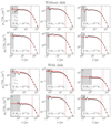 |
Fig. A.1. Final 3D density profiles of the clumps in the spherical-host simulations presented in Sect. 5.1 (first two rows) and for the case in which the external potential also includes a Sparkler-like stellar disc as described in Sect. 5.2 (last two rows). First and third row: Clumps with mass 106.3 M⊙, 106.6 M⊙, and 106.9 M⊙ (left, central, and right panels, respectively). Second and fourth row: Clumps with mass 107.2 M⊙, 107.5 M⊙, and 107.8 M⊙ (left, central, and right panels, respectively). The black dots are the N-body density profiles, while the red solid line is the best-fit Plummer density profile (with the shaded are marking the 1σ, 2σ, and 3σ confidence levels), as described in Appendix A. The grey shaded area highlights the region within the softening length, that is excluded from the fit. The grey dashed line is the initial Plummer scale radius rs, i, and the red dashed line is the best-fit final scale radius rs, f. |
Appendix B: Tidal stripping in elliptical orbits
In Sect. 5.1 we have shown the tidal stripping history of clumps of different mass in circular orbit at 1 kpc from the centre of the Sparkler-like spherical halo, modelled with an external gravitational potential. This setup implies that the clumps are not affected by dynamical friction and do not deviate from their initial orbit. We have chosen this setup in order to maximise the tidal stripping effects, initialising the clumps as close as possible to the threshold that, according to our definition, divides surviving and lost clumps. The results presented in Sect. 5.1 show that the fraction of tidal mass losses are not sufficient to make the mass of Sparkler-like clumps comparable to local GCs. That is why in Sect. 5.2 we introduced the Sparkler stellar disc as an external potential, in order to trigger tidal shocks and substantially enhance the amount of stripped stars.
In this Appendix we explored the differences arising in the setup of Sect. 5.1 when we consider non-circular orbits and the dragging effect of dynamical friction in the spherical halo. To choose the orbital parameters, we selected six clumps from the 30 runs discussed in Sect. 4.4.3, choosing surviving clumps of different masses that at the end of the simulation are at a distance slightly larger than 1 kpc. In Table B.1 we list their initial conditions, while in Fig. B.1 we compare their initial and final positions with those of the other surviving clumps.
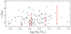 |
Fig. B.1. Final distance of the surviving clumps (black dots) for all the simulations with point-mass clumps in a halo made of particles in the case of the spherical configuration (Sect. 4.4.3). The red crosses and lines show the initial and final distance of the six clumps studied in this section. The grey dotted line is at 1 kpc, the threshold that divides the surviving and the lost clumps. |
The dynamical friction is natively present in the simulations of Sect. 4.4.3, while in a setup like the one of Sect. 5.1 it must be implemented via semi-analytical models. Therefore, we modelled the dynamical friction deceleration of the clump centre of mass using the Chandrasekhar formula (Chandrasekhar 1943; Binney & Tremaine 2008):
![Mathematical equation: $$ \begin{aligned} \boldsymbol{a}_\mathrm{DF} (\boldsymbol{x})=-2\pi G^2 M_*\,\rho _\mathrm{halo} (\boldsymbol{x}_\mathrm{CM} )\,\ln \Lambda \left[\mathrm{erf} (X)-\frac{2X}{\sqrt{\pi }}\exp (-X^2)\right]\frac{\boldsymbol{v}_\mathrm{CM} }{|\boldsymbol{v}_\mathrm{CM} |^3}. \end{aligned} $$](/articles/aa/full_html/2025/09/aa54669-25/aa54669-25-eq69.gif) (B.1)
(B.1)
In Eq. B.1M* is the clump stellar mass, ρhalo is the halo density,  and
and  are the position and the velocity of the clump centre of mass, respectively.
 ![Mathematical equation: $ X=|\boldsymbol{v}_{\mathrm{CM}}|/[\sigma_r(|\boldsymbol{x}_{\mathrm{CM}}|)\sqrt{2}] $](/articles/aa/full_html/2025/09/aa54669-25/aa54669-25-eq72.gif) , where σr is the radial velocity dispersion of the background (that is analytical for a Hernquist isotropic system, Hernquist 1990). Λ is a constant that goes into the Coulomb logarithm, and it can computed as
, where σr is the radial velocity dispersion of the background (that is analytical for a Hernquist isotropic system, Hernquist 1990). Λ is a constant that goes into the Coulomb logarithm, and it can computed as
 (B.2)
(B.2)
with rhm being the clump half-mass radius and γ = |dlnρhalo/dlnr| or fixed arbitrarily (Petts et al. 2016). At each time step, this acceleration is added to each particle of the resolved clump. We fixed the clump mass to its initial value and we tuned the value of lnΛ for each clump in order to qualitatively reproduce the orbits of the chosen clumps in the simulations of Sect. 4.4.3. The values of lnΛ are listed in Table B.1, while in Fig. B.2 we show the comparisons between the orbits of the chosen point-mass clumps as derived from Sect. 4.4.3 and the one obtained with the Chandrasekhar formula.
Parameters of the six clumps chosen to test the effects of orbit eccentricity and dynamical friction on tidal stripping.
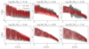 |
Fig. B.2. Orbits of the clumps under the effect of dynamical friction. For each panel, the black solid line represents the orbit of the selected clump (parameters in Table B.1) in the simulation of point-mass clumps in a spherical halo made of particles for the spherical configuration (Sect. 4.4.3). The red dashed line indicates the orbit of the same clump in the same halo but implemented as an external potential and with the addition of the Chandrasekhar formula, as described in Appendix B. |
In Table B.1 we also list the fraction of residual mass of the six chosen clumps of this section, compared with the fraction of residual mass of clumps of similar mass in the cases without and with a disc (Sects. 5.1 and 5.2). Comparing the results with those obtained previously, it turns out that in four out of six cases the tidal stripping is consistent with or less efficient than the one derived for the 1-kpc circular orbits in the spherical case. This is most likely due to the fact that the clumps do not start the simulation in the innermost regions of the system, reaching them only by the end of the run because of the sinking effect of dynamical friction. The only exceptions are clumps 1 and 4, that retain 72% and 82% of their initial mass, while the retained mass fractions in the case of circular 1-kpc orbit are 84% and 87%, respectively. We find that the orbits of these two clumps have the largest eccentricity among the six explored, with e = (a − b)/(a + b)≈0.6, where a and b are the apocentre and pericentre of the orbit, respectively. Therefore, it is possible that the clump, spanning a wider range of distances during its orbit, may experience a larger gravitational field gradient, resulting in an increased tidal stripping. However, such an increase (≈10% of additional lost mass at best) is negligible if compared with the effects of tidal shocks. Indeed, the predicted residual mass in presence of a disc is smaller than the one obtained for the six clumps studied in this section. This comparison demonstrates that the eccentricity of the orbits and the dynamical friction are second-order effects compared to the presence of the disc, especially in our experiments that are aimed at maximising the tidal losses of the over-massive Sparkler clumps.
All Tables
Best-fitting parameters of the mass distributions for the initial (third column) and survived (fourth-to-sixth columns) samples of clumps.
Best-fitting parameters of the distance distributions for the initial (first row) and survived (second row) samples of clumps.
Parameters of the Sparkler-like exponential disc (first row) and of the three MN disks (second, third, and fourth rows) that, summed together, better approximate the potential of the original exponential disc (see Smith et al. 2015).
Parameters of the six clumps chosen to test the effects of orbit eccentricity and dynamical friction on tidal stripping.
All Figures
|
Fig. 1. Size-mass relation for the extraplanar clumps of the Sparkler galaxy (Sect. 2). Clumps are shown as black empty circles, while the best-fitting line (obtained as described in Sect. 2.1) is plotted as the red solid line. The red shaded areas (from opaque to transparent red) show the 1σ, 2σ, 3σ intervals of the fit, respectively. |
| In the text | |
|
Fig. 2. Top panel: Density profile of the highest-mass DM halo of the Sparkler galaxy as predicted by the models by Correa et al. (2015). Black lines indicate the z = 0 profile while red lines the z = 1.378 one. The dotted lines mark r−2, the dashed lines mark r200. The grey shaded area marks the region between 1 and 10 kpc, that is the interval under study. Bottom panel: Difference between the halo density profile at z = 0 and at z = 1.378 normalised to the density profile at z = 0. |
| In the text | |
|
Fig. 3. Dynamical-friction timescales for clumps of mass 106, 107, and 108 M⊙ (dashed, dotted and solid lines, respectively) as a function of the distance from the centre of the halo. The red-dashed area covers the range of dynamical friction timescales relative to the interval of clump masses and distances of interest. The grey horizontal line corresponds to the look-back time at z ≈ 1.4 tlb = 9.23 Gyr, that divides the plot between the region in which the dynamical friction is most likely inefficient (tfric > 9.23 Gyr) and efficient (tfric < 9.23 Gyr). The latter is marked by the grey area. |
| In the text | |
|
Fig. 4. Left panel: Evolution over 9.23 Gyr of the distances from the centre of the point-mass clumps orbiting in a Sparkler-like potential with circular orbit initial conditions. On the x-axis, the mass of the clump is reported, and the black arrows point from the initial to the final distance. The final distance is computed as the average distance from the centre of the system, within the last 5% of the simulated time. The masses larger than the vertical dotted grey line are also larger than the observed stellar masses of the Sparkler clumps. We classify as survived the clumps with final distance out of the shaded area. Right panel: Colour map of the final distance of the clumps as a function of their initial distance (y-axis) and dynamical mass (x-axis), obtained by interpolating the simulations shown in the left panel. The colour bar traces the final distance and goes from 1 kpc (or less) to 6 kpc (the largest simulated initial distance). The contours mark the combinations of initial distance and mass that result in specific values of final distance (from 1 to 5 kpc). The green data points are the extraplanar Sparkler clumps (Claeyssens et al. 2023; Forbes & Romanowsky 2023). For each clump three distances are computed, de-projecting the observed distances depending on the three spatial configurations studied in Sect. 2.4 (face-on disc, edge-on disc, and spherical), as described in Sect. 4.2. The symbols (squares and crosses) indicate the median of the three possible distances, with the error-bars corresponding to the minimum and maximum distance. We used squares for the clumps that survive, while we used crosses for the clumps for which the inferred final distance is smaller than 1 kpc. |
| In the text | |
|
Fig. 5. Initial spatial distribution of the ten clumps in representative simulations of the three different spatial configurations described in Sect. 2.4. The initial positions of the clumps are determined as described in Sect. 4.3. From left to right: Face-on disc, Edge-on disc, and Spherical configurations. Each clump is displayed as a coloured dot. In the first two panels, we plot in grey the trajectory of the circular orbit at which each clump is initialised. This also makes apparent that the orbits of the clumps are co-planar in these two configurations. In the right panel, for each clump we plot the projected distance on the x − y plane as the black solid line, and the z coordinate of the clump as the red dotted line, to show that the clumps are not co-planar. |
| In the text | |
|
Fig. 6. Fraction of survived clumps of each of the 30 simulations run in the face-on (top panel, in red), edge-on (middle panel, in green) and spherical (bottom panel, in blue) configurations. A clump is flagged as survived if its distance from the centre of the halo at the end of the simulation is larger than 1 kpc. The vertical solid line and the shaded area show the median fraction of survived clumps |
| In the text | |
|
Fig. 7. Fraction of initial clumps and survived clumps per mass-bin, shown as grey histograms and coloured histograms (red for the face-on configuration, green for the edge-on configuration and blue for the spherical configuration), respectively. We show the face-on configuration in the top panel, the edge-on configuration in the middle panel, the spherical configuration in the bottom panel. The histograms are built binning all the clumps (either initial or survived) of the 30 simulations, normalised to the initial total number of clumps (ten for each simulation, therefore 300). The black and coloured lines are the best-fitting Gaussian distributions, of which we report the mean in the legend. |
| In the text | |
|
Fig. 8. Surface number density profiles of the clumps in the face-on (top panel), edge-on (middle panel), and spherical configuration (bottom panel). In each panel, the dark grey line is the initial distribution, with the grey shaded areas covering the 1σ and 2σ intervals, built adopting the corresponding function described in Sect. 2.4 with the best-fit parameters listed in the first row of Table 3. We projected all the profiles along the z axis. The triangles show the profiles of the initial clump positions in the x − y plane, computed stacking together the 10 clumps in all the 30 runs. The coloured hexagons show the surface number density profiles at the end of the simulations, obtained stacking together all the survived clumps. The corresponding coloured solid line is the best-fit profile to the final projected distances of the survived clumps, obtained as described in Sect. 4.4. We normalised all the profiles to the total number of initial clumps, so the integral of the initial profiles is equal to 1, and the integral of the survived profiles is equal to the average surviving fraction (distributions shown in Fig. 6). |
| In the text | |
|
Fig. 9. Fraction of the clump mass enclosed within the tidal radius defined as in Eq. (14). The masses of the clumps are 106, 107, and 108 M⊙ (dashed, dotted and solid lines, respectively). The effective radius of the clumps is given by Eq. (1). Tidal radii are computed for distances between 1 and 10 kpc. |
| In the text | |
|
Fig. 10. Top panel: Retained mass (relative to the initial one) as a function of time for clumps of different masses in circular orbits at 1 kpc from the centre of the system. The residual mass is computed within 4rs, where rs is the initial Plummer scale radius. In this case, the clumps orbit in a Sparkler-like spherical potential representing the total mass, defined in Sect. 4.1. Masses go from log(M*/M⊙) = 6 to log(M*/M⊙) = 7.8 with a step of 0.3 dex (the arrow points from the smallest to the highest mass). Bottom panel: Same as the left panel but for clumps in quasi-circular orbit at 1 kpc from the centre of the system including a stellar disc component (modelled as in Sect. 5.2). The clump orbital plane is inclined of 30 degrees with respect to the plane of the disc. |
| In the text | |
|
Fig. 11. Comparison between the initial conditions and the snapshot at 0.51 Gyr for the tidal-shock simulation described in Sect. 5.2 in the case of mass M* = 106 M⊙. The top and bottom panels show the projections on the x − y and x − z planes, respectively. The clump stellar particles are shown as red and black dots for the snapshots at t = 0 Gyr and t = 0.51 Gyr, respectively. The centres of clumps at t = 0 Gyr and t = 0.51 Gyr are shown as a black and red star, respectively, with an horizontal line of length 4 rs, i, where rs, i is the initial Plummer scale radius. The grey dashed curves represent the trajectory of the clump. The orange curves trace iso-density contours of the Sparkler disc external potential. The centre of the system is marked by a black cross. |
| In the text | |
|
Fig. 12. Comparison between the final (rs, f) and initial (rs, i) scale radii of the clumps simulated in Sect. 5 when modelled as a Plummer sphere, as in Eq. (15). The initial scale radii are computed from the size-mass relation of Sect. 2.1. The final scale radii are obtained fitting a Plummer density profile to the final snapshots of the simulations of resolved clumps in a spherically symmetric Sparkler-like system (Sect. 5.1, circles) and of the simulations including the effects of a disc (Sect. 5.2, triangles). The dashed line is the 1 : 1 relation. |
| In the text | |
|
Fig. 13. Left panel: Fraction of the clump mass lost after 9.23 Gyr |ΔM*, fin|/M*, ini as a function of the initial mass M*, ini. Here ΔM*, fin = M*, fin(4rs)−M*, ini, where M*, fin(4rs) is the final mass within four initial Plummer scale radii, computed as in Sect. 5.2. The circles are the results from the simulations of resolved clumps described in Sect. 5.2, while the line is the best fit (Eq. 17) and the shaded area is the 1σ interval. Right panel: Distributions of the number of clumps per mass bin, normalised to the total initial number of clumps. The grey and blue histograms are the analogues of those shown in the bottom panel of Fig. 7, and they show the initial and surviving number of clumps, respectively, in the spherical configuration case considering the effects of dynamical friction only. The purple histogram shows the mass distribution of the surviving clumps of scenario 1 (short dynamical-friction timescale; Sect. 5.2), while the golden histogram shows the mass distribution of the surviving clumps of scenario 2 (short tidal-stripping timescale; Sect. 5.2). A Gaussian function is fitted to each histogram and shown with the corresponding colour. |
| In the text | |
|
Fig. A.1. Final 3D density profiles of the clumps in the spherical-host simulations presented in Sect. 5.1 (first two rows) and for the case in which the external potential also includes a Sparkler-like stellar disc as described in Sect. 5.2 (last two rows). First and third row: Clumps with mass 106.3 M⊙, 106.6 M⊙, and 106.9 M⊙ (left, central, and right panels, respectively). Second and fourth row: Clumps with mass 107.2 M⊙, 107.5 M⊙, and 107.8 M⊙ (left, central, and right panels, respectively). The black dots are the N-body density profiles, while the red solid line is the best-fit Plummer density profile (with the shaded are marking the 1σ, 2σ, and 3σ confidence levels), as described in Appendix A. The grey shaded area highlights the region within the softening length, that is excluded from the fit. The grey dashed line is the initial Plummer scale radius rs, i, and the red dashed line is the best-fit final scale radius rs, f. |
| In the text | |
|
Fig. B.1. Final distance of the surviving clumps (black dots) for all the simulations with point-mass clumps in a halo made of particles in the case of the spherical configuration (Sect. 4.4.3). The red crosses and lines show the initial and final distance of the six clumps studied in this section. The grey dotted line is at 1 kpc, the threshold that divides the surviving and the lost clumps. |
| In the text | |
|
Fig. B.2. Orbits of the clumps under the effect of dynamical friction. For each panel, the black solid line represents the orbit of the selected clump (parameters in Table B.1) in the simulation of point-mass clumps in a spherical halo made of particles for the spherical configuration (Sect. 4.4.3). The red dashed line indicates the orbit of the same clump in the same halo but implemented as an external potential and with the addition of the Chandrasekhar formula, as described in Appendix B. |
| In the text | |
Current usage metrics show cumulative count of Article Views (full-text article views including HTML views, PDF and ePub downloads, according to the available data) and Abstracts Views on Vision4Press platform.
Data correspond to usage on the plateform after 2015. The current usage metrics is available 48-96 hours after online publication and is updated daily on week days.
Initial download of the metrics may take a while.