| Issue |
A&A
Volume 701, September 2025
|
|
|---|---|---|
| Article Number | A125 | |
| Number of page(s) | 7 | |
| Section | Catalogs and data | |
| DOI | https://doi.org/10.1051/0004-6361/202555675 | |
| Published online | 09 September 2025 | |
Catalogue of central stars of extragalactic planetary nebulae
1
Universidad Nacional de Córdoba, Observatorio Astronómico de Córdoba,
Laprida 854,
X5000BGR
Córdoba,
Argentina
2
Consejo Nacional de Investigaciones Científicas y Técnicas (CONICET),
Godoy Cruz
2290, CABA, CPC 1425FQB,
Argentina
3
Instituto de Astrofísica de La Plata, Consejo Nacional de Investigaciones Científicas y Técnicas Avenida Centenario (Paseo del Bosque) S/N,
B1900FWA
La Plata,
Argentina
4
Institut für Astronomie und Astrophysik, Kepler Center for Astro and Particle Physics, Eberhard Karls Universität,
Sand 1,
72076
Tübingen,
Germany
5
Instituto de Astronomía Teórica y Experimental (IATE, CONICET-UNC),
Laprida 854,
X5000,
Córdoba,
Argentina
★ Corresponding author: This email address is being protected from spambots. You need JavaScript enabled to view it.
Received:
27
May
2025
Accepted:
19
July
2025
Abstract
Context. Central stars of planetary nebulae (CSPNe) are essential for understanding the final evolutionary stages of low- and intermediate-mass stars. However, their study in extragalactic environments remains challenging due to their intrinsic faintness and the limited availability of high-quality data.
Aims. We aim to provide a comprehensive and up-to-date catalogue of extragalactic CSPNe in order to enable a more complete view of their physical properties across different galactic environments and metallicities.
Methods. The catalogue was assembled using data from the most recent and reliable literature sources. Priority was given to collecting effective temperatures and luminosities that have either been directly reported or consistently derived. When available, spectral types or specific spectral features – such as P-Cygni profiles or broad Hα emission lines – were also included. This approach allowed for broader characterisation of the sample, even when accurate classifications are not available.
Results. We present a new compilation of extragalactic CSPNe – the largest to date – comprising over 800 objects located in the Magellanic Clouds, NGC 300, NGC 5128, and fifteen other nearby galaxies. This catalogue enables, for the first time, a global comparison of CSPNe physical parameters beyond the Milky Way. Updated Hertzsprung–Russell diagrams are provided featuring CSPNe from seven different galaxies, revealing trends and outliers that merit further investigation. The catalogue represents a valuable resource for future spectroscopic follow-up and for improving our understanding of post-AGB evolution in diverse galactic contexts.
Key words: catalogs / stars: evolution / planetary nebulae: general / Local Group
© The Authors 2025
 Open Access article, published by EDP Sciences, under the terms of the Creative Commons Attribution License (https://creativecommons.org/licenses/by/4.0), which permits unrestricted use, distribution, and reproduction in any medium, provided the original work is properly cited.
This article is published in open access under the Subscribe to Open model. This email address is being protected from spambots. You need JavaScript enabled to view it. to support open access publication.
1 Introduction
Planetary nebulae (PNe) represent a brief phase in the evolution of low- and intermediate-mass stars, i.e. those with masses between 0.8 and 8.0 M⊙. Within the standard single stellar evolution scenario, PNe are formed when the progenitor star ejects most of its envelope and the remaining stellar remnant contracts and heats up. During this stage, the previously ejected material is ionised by the central star, producing the characteristic glowing structure (Kwok 2007; Kwitter & Henry 2022). The central stars of planetary nebulae (CSPNe) play a fundamental role in shaping the morphology and evolution of PNe. Additionally, they serve as valuable probes of stellar evolution, providing insight into the properties of stellar populations and the chemical composition of their host environments.
In the Milky Way (MW), extensive efforts have been made to catalogue PNe and their central stars. A key contribution to the latter is the compilation by Weidmann & Gamen (2011); Weidmann et al. (2020); González-Santamaría et al. (2021), which made it possible to assess the detectability of CSPNe. That catalogue showed that only about ~21% of CSPNe can be identified and characterised in terms of their properties, such as temperature and luminosity, due to observational challenges and intrinsic faintness. Additionally, Weidmann et al. (2020) found that 50% of the sample (88 out of 175 objects) with derived values of luminosity (L), effective temperature (Tef f), and surface gravity (g) have masses and ages consistent with single stellar evolution models, suggesting that some single stars are indeed capable of forming PNe.
Due to their brightness, PNe can be detected in other galaxies. Notably, Jacoby (1989) and Ciardullo et al. (1989) demostrated that PNe can serve as distance calibrators through the planetary nebula luminosity function (PNLF). Significant efforts have been devoted to identifying PNe in other galaxies, leading to the discovery of several thousand extragalactic PNe (e.g. Ford et al. 2002; Magrini 2006). Moreover, intracluster PNe have even been detected (e.g. Arnaboldi et al. 2007; Spiniello et al. 2018).
The study of PNe in extragalactic environments offers a complementary perspective to that of the MW, helping to clarify how factors such as metallicity and star formation history influence stellar evolution (Jacoby & Ciardullo 1999; Stanghellini & Haywood 2010; Valenzuela et al. 2025). Extragalactic PNe have been identified in galaxies such as the Magellanic Clouds (Reid & Parker 2010a), M 31 (Merrett et al. 2006), and M 33 (Ciardullo et al. 2004), providing unique data on stellar evolution across different galactic environments. However, characterising the extragalactic CSPNe is more challenging due to their low luminosity and the distances involved (Gesicki et al. 2018).
Despite these challenges, the growing amount of published data opens the possibility of consolidating existing information into a unified catalogue. Previous efforts, such as the most recent catalogue of CSPNe by Weidmann et al. (2020), have demonstrated the value of systematic data collection in enabling robust statistical and comparative studies.
In this work, we present a compilation of inferred properties of extragalactic CSPNe. In particular, we focus on their Tef f, L, and (when available) their spectral type (SpT). While the spectral type provides essential information about the evolutionary status of these stars, obtaining it is particularly challenging due to the low brightness of the targets. As a result, the properties of a significant part of these central stars – such as L, Tef f, and even spectral classification – have been inferred through modelling efforts rather than direct observations. This catalogue integrates data from direct measurements and models, offering a valuable resource for investigating how the properties of central stars vary across different galactic environments. We expect this catalogue to serve as a foundation for future observational and theoretical studies on stellar evolution across diverse environments.
While the primary objective of this work is to provide a comprehensive compilation of candidate CSPNe, we acknowledge that not all objects included can be considered confirmed PNe. Similarly, the derived or compiled stellar parameters (e.g. effective temperature and luminosity) should be treated with caution. Given the limitations and heterogeneity of the available data, we emphasise that this catalogue is intended as a resource for exploratory analysis and future observational follow-up, rather than as a definitive dataset for deriving robust correlations with metallicity or progenitor mass.
The structure of this paper is as follows. In Section 2 we provide a detailed description of the catalogue and discuss its limitations, while in Section 3, we analyse and discuss the distribution of the physical parameters of the extragalactic PNe. Finally, the discussion and conclusions are presented in Sections 4 and 5.
2 The catalogue of extragalactic CSPNe
The main objective of this work is to compile known properties of extragalactic CSPNe, including the spectral type (SpT), log(L/L⊙), and log(Tef f). The catalogue includes 1073 objects across 19 galaxies. Table 1 presents the main characteristics of these galaxies. Nearly all the galaxies included, except M 81, NGC 5128, NGC 300, and NGC 5236, are members of the Local Group. This underscores the substantial volume of extragalactic PNe with available spectroscopic data.
While the catalogue provides a comprehensive list of CSPNe, only a few of the entries include references to spectral type, with the majority of these objects located in the Large Magellanic Cloud (LMC).
Data were gathered from refereed publications post 1985. For objects with multiple determinations, we report the most recent values. Information in the catalogue, organised by galaxy and right ascension (RA), includes the following:
Col. 1: name of the PN, prioritising the designation used in the original publication from which the data was obtained.
Col. 2: host galaxy.
Cols. 3–4: the RA and DEC as listed in the original publications, with minimal differences from the Centre de Données astronomiques de Strasbourg (CDS).
Cols. 5–6: logarithm of the CSPN’s effective temperature (log Tef f) and its reference. In some galaxies, data for the central star were unavailable. However, the emission line intensities of the PNe that could be identified have been reported in the literature. In these cases, we were able to estimate the temperature (see Sect. 3.3).
Cols. 7–8: logarithm of the luminosity, in units of solar luminosity (log L/L⊙), and reference source. In the same way as for the temperature, we have been able to compute the luminosity using the magnitude of the nebula at [O III]λ5007 (see Sect. 3.3).
Cols. 9–10: spectral type and reference. In cases where the spectral type was not explicitly listed, additional information (e.g. P Cygni profiles, broad Hα emission) helped us infer the characteristics.
Col. 11: references identifying the CSPN as a binary system.
Col. 12: comments.
The coordinates have been rounded to the nearest tenth or to ‘.00’ where precision is lacking. We followed the same criterion for log(L/L⊙) and log(Tef f). While errors for the physical parameters are sometimes given in the original publications, they are not included in this catalogue. We provide a discussion on uncertainties in Sect. 2.1.
2.1 A few caveats
As mentioned earlier, only a few extragalactic CSPNe have a spectral classification. Detecting an O(H) star is challenging due to their faint absorption lines, which require a high signal-to-noise (S/N) spectra. In contrast, Wolf–Rayet ([WR]) stars are easier to identify even with a lower S/N in the continuum, as their strong emission lines are prominent. Indeed, in this catalogue, the vast majority of CSPNe with a determined spectral type are [WR]. For all reported objects, the parameters of the central star were estimated from the observed nebular spectra. While most properties were primarily inferred using Cloudy models (Ferland et al. 1998, and references therein), in some cases, the Zanstra temperature was also determined (e.g. Villaver et al. 2004). This limitation directly affects the accuracy of stellar parameter determinations. Moreover, in most cases, only low-quality spectra are available, thus only allowing for an estimation of temperature and luminosity (see Sect. 3.3). The most reliable approach to accurately obtaining physical parameters for CSPNe is through fitting stellar atmosphere models to their spectra (e.g. Mendez et al. 1988). To illustrate the uncertainties associated with the stellar parameters listed in our catalogue, Table 2 presents examples of extragalactic CSPNe with varying determinations of these physical parameters. In addition, in Section 3.5 we present a discussion on the uncertainties associated with two specific methods.
Another crucial aspect to consider is that the objects in this catalogue should be regarded as PN candidates, even if the paper does not explicitly state this. These objects are poorly studied, and in most cases there is only a single spectrum available. Especially considering that PNe are perhaps one of the most difficult objects to classify, their status only as candidates should not be overlooked (Frew & Parker 2010). Additional considerations must also be addressed. Murset & Nussbaumer (1994) proposed an empirical relationship between the temperature of the ionising source (T*) in a photoionised gaseous nebula and the highest observed ionisation potential (χi):
![Mathematical equation: $\[T_*=\chi_i \times 1000 \qquad[K / e V].\]$](/articles/aa/full_html/2025/09/aa55675-25/aa55675-25-eq1.png) (1)
(1)
In general, extragalactic PNe are identified by means of the interferential filter centred on [O III]λ5007. In this context, the temperatures of the extragalactic CSPNe of our catalogue will be higher than 35 100 K.
Another point to consider is that extragalactic PNe are detected as point sources due to the great distance separating us from them, which prevents their actual extent from being determined and makes it impossible for their surface brightness to be discerned. In this sense, what is actually detected is their integrated brightness. A reasonable assumption that only the brightest PNe are detected. This, in turn, implies that these PNe have bright central stars. Additionally, their nebulae are not too diffuse, making them optically thick and thus favouring their detection. Moreover, according to Ciardullo et al. (2005), the progenitors of the PNe that populate the top 0.5 mag of the PNLF (i.e. the brightest PN) have core masses of ≳0.6 M⊙. Nevertheless, we cannot infer realistic masses with the data currently available and collected in this catalogue. In summary, in the extragalactic context, only the most luminous CSPNe in compact and optically thick nebulae will be detectable.
Finally, given that all the compiled candidate PNe must be relatively bright, it is expected that they are in an early stage of CSPNe evolution. Specifically they are in the flat region of their evolutionary tracks, which is before they begin to lose luminosity as they cool down (see the evolutionary tracks of Miller Bertolami 2016).
Main parameters of the galaxies in our sample. Namely, these are galaxy name, number of catalogued PNe, metallicity, morphological type, color, and global stellar mass.
Some objects with different determinations in their physical parameters.
3 Analysis of physical parameters
To compare the distribution of the physical parameters of our CSPN sample with those of the MW, we used the data from the Weidmann et al. (2020) catalogue. The objects that are known to be binary were not considered. Fig. 1 shows the HR diagram, and H-rich and H-poor CSPNe appear to be evenly intermingled. Consequently, in the following figures, no distinction is made between H-rich and H-poor. It is worth noting that the physical parameters of CSPNe in our Galaxy were generally determined using stellar atmosphere models, whereas for extragalactic CSPNe, this method is unfeasible (see Sect. 2.1).
3.1 LMC and SMC
Figure 2 shows log(Tef f) versus log(L/L⊙) for the LMC and Small Magellanic Cloud (SMC) galaxies along with the sample of CSPNe from the MW previously described. This is the most complete HR diagram of CSPNe to date for these two galaxies. The data for the LMC and SMC were collected from eleven different articles, resulting in variations in the methods used to derive the physical parameters. We note that this may affect the comparison between the different samples in Fig. 2 given that the physical parameters were not determined using the same methodologies.
Figure 2 highlights that the point distributions of the LMC and SMC are well mixed. Although the metallicities of the two galaxies (Table 1) are quite different, the quality of the data does not allow us to draw any conclusion about a possible trend with metallicity.
Nevertheless, the CSPNe of our most important satellite galaxies occupy the same region of the HR diagram as the CSPNe in our own Galaxy. Although the point cloud of the MW is somewhat shifted towards lower temperatures compared to the points in the LMC and SMC, this is likely attributable to the methodology used for the detection of extragalactic PNe (see comments related to Eq. (1)). Additionally, we note that we did not detect PNe with white dwarfs (WD) nuclei. This makes perfect sense, as PNe with WD nuclei are objects with low intrinsic luminosities. Notably, the most luminous CSPNe candidates are found in the Magellanic Clouds (Fig. 2).
In Fig. 2, two regions in the HR diagram that feature high values of temperature and luminosity are indicated. While some objects in these regions are classified as probable PNe or confirmed binaries, others are not. In the high-luminosity region, these sources are unlikely to be CSPNe. According to Miller Bertolami (2016), the most luminous CSPNe reach up to log(L/L⊙) ≃ 4.4, but even in such cases, they would correspond to massive CSPNe with extremely rapid evolution, making them very difficult to detect. Alternatively, these objects might instead be classical WR stars (see Fig. 2 of Shenar 2024).
As for the objects located in the high-temperature region, they could potentially be CSPNe. Incidentally, they would be among the most massive ones. Such a population of very massive CSPNe could be the progeny of high mass stars formed recently (<1 Gyr) in the Magellanic Clouds (Harris & Zaritsky 2009; Mazzi et al. 2021). Again, such objects evolve quickly, making them difficult to detect. In any case, the sources in this region should be studied in more detail, as we might be looking at a very peculiar CSPN.
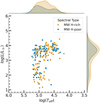 |
Fig. 1 Hertzsprung–Russell diagram showing CSPNe within the MW from Weidmann et al. (2020). The marginal curves represent the data using a continuous probability density curve. |
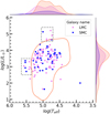 |
Fig. 2 Hertzsprung–Russell diagram of CSPNe in the LMC and SMC. The coldest CSPN in the SMC likely has poorly constrained parameters, as an effective temperature (Teff) above 10 000 K is required to efficiently ionise hydrogen. The orange contour shows the distribution of points for the MW. In grey, two regions with extreme values are highlighted (see text for details). |
3.2 The case of NGC 300
Soemitro et al. (2023) obtained spectroscopic data from a moderate sample of PN in NGC 300. This allowed them to obtain an estimate for the temperature and luminosity of the CSPNe.
The effective temperatures of the CSPNe in NGC 300 were estimated using the empirical excitation class (EC) method defined by Reid & Parker (2010b) as follows:
![Mathematical equation: $\[E C_{low}=0.45\left[\frac{F(5007)}{F(H \beta)}\right]\]$](/articles/aa/full_html/2025/09/aa55675-25/aa55675-25-eq3.png) (2)
(2)
![Mathematical equation: $\[E C_{h i g h}=5.54\left[\frac{F(4686)}{F(H \beta)}+\log _{10} \frac{F(4959)+F(5007)}{F(H \beta)}\right] \text {, }\]$](/articles/aa/full_html/2025/09/aa55675-25/aa55675-25-eq4.png) (3)
(3)
where EClow applies for 0 < EC < 5 and EChigh for 5 ≤ EC < 12. Therefore, the empirical relationship between the excitation class and effective temperature is
![Mathematical equation: $\[\log \left(T_{e f f}\right)=4.439+[0.1174(E C)]-\left[0.00172\left(E C^2\right)\right].\]$](/articles/aa/full_html/2025/09/aa55675-25/aa55675-25-eq5.png) (4)
(4)
A peculiarity of this temperature estimation method is the discontinuity between Eqs. (2) and (3). As a result, applying it to a large sample of objects may produce an artificial gap in the temperature distribution. It is important to mention that these equations are valid if the nebula is optically thick. In addition, the datasets used did not cover the wavelength range including the He II λ4686 line, which is essential for determining medium- and high-excitation classes. As a result, the effective temperatures (Tef f) for excitation classes greater than 5 (EC ≥ 5) could only be estimated as lower limits, with log(Tef f) ≳ 5. Conversely, for objects with EC < 5, log(Tef f) < 5 is expected.
On the other hand, for luminosity estimates, Soemitro et al. (2023) assumed that ~11% of the CSPN’s luminosity is efficiently converted into the [O III]λ5007 emission line. This implies that a significant fraction of the CSPN’s energy is channeled into this specific line (e.g. Dopita et al. 1992; Schönberner et al. 2010). This assumption is as follows:
![Mathematical equation: $\[L_{5007}=4 \pi d^2 F_{5007},\]$](/articles/aa/full_html/2025/09/aa55675-25/aa55675-25-eq6.png) (5)
(5)
![Mathematical equation: $\[L_{5007}=0.11 L_*.\]$](/articles/aa/full_html/2025/09/aa55675-25/aa55675-25-eq7.png) (6)
(6)
This assumption holds for optically thick nebulae and when [O III]λ5007 is the only coolant. If the nebula is optically thin, the efficiency of this ion decreases, meaning the estimated luminosities represent lower limits, similar to Tef f, thus making it difficult to impose stricter constraints on CSPN masses. In this sense, Soemitro et al. (2023) combines Eqs. (5) and (6).
The proportionality constant of Eq. (6) depends on factors such as the CSPN mass and the (O/H) abundance (Schönberner et al. 2010) as well as whether it is hydrogen-burning or helium-burning (Jacoby 1989) and the Tef f (Dopita et al. 1992).
In summary, as outlined in Soemitro et al. (2023), this represents a lower limit for luminosity and effective temperature. This premise is reflected in the HR diagram of Fig. 3, where many CSPNe fall in the low-L (log(L/L⊙) < 2.5) and low-Tef f (log(Tef f) < 5.1) region, where the nebulae have nearly disappeared and only white dwarfs are observed (see Fig. 9 of Weidmann et al. 2020).
3.3 The case of M 81, NGC 185, NGC 3109, and NGC 5128
The emission line intensities of numerous PNe in some well-studied galaxies have been reported in the literature: M 81 (Stanghellini et al. 2010), NGC 185 (Richer & McCall 2008), NGC 3109 (Flores-Durán et al. 2017), and NGC 5128 (Walsh et al. 2015). Using the [O III] and He II lines, we calculated the EC to estimate the effective temperature of the CSPNe, following the method applied by Soemitro et al. (2023), Eqs. (2), (3), and (4). This method requires the nebula to be optically thick. To determine if the nebulae is optically thick, we used the criteria as proposed by Soemitro et al. (2023):
![Mathematical equation: $\[F(6584) / F(H \alpha)>0.3.\]$](/articles/aa/full_html/2025/09/aa55675-25/aa55675-25-eq8.png) (7)
(7)
For M 81 and NGC 185, we excluded optically thin objects from our catalogue. Unfortunately, the intensity of the [N II]λ6584 line for objects in NGC 5128 has not been published. In this case, as we do not know the optical depth of the PNe in the sample, we assumed that they are all optically thick. Similarly, although the line intensities of PNe in NGC 3109 have been published (Flores-Durán et al. 2017), these objects were excluded from our catalogue due to their optically thin nature.
As long as the [O III]λ5007 and Hβ lines are visible, the EC can be calculated through both Eqs. (2) and (3). To decide which to apply, we adopted the following criterion: If emission from He IIλ4686 is reported, we use Eq. (3); otherwise, we apply Eq. (2). To compute the EC of the PNe in NGC 5128, we used the approximation F(5007) = 3.01 F(4959) (Acker et al. 1989), as the intensity of the 4959 Å line is not reported for these PNe.
On the other hand, according to the Eq. (1), a temperature of 54 400 K is required to produce He II emission. Moreover, Eq. (4) indicates that an EC greater than ~2.63 is necessary for He II emission. Thus, if Eq. (2) yields an EC lower than 2.6 but He II emission is observed, we attribute this emission to the central star and mark it as “[WR]?”.
Three objects in NGC 5128 (namely, P04_4609, EMMI_480, and EMMI_2045) exhibit an EC > 12, which we interpret as indicative of stellar emission. Although these objects are undoubtedly very hot, we did not assign them a specific temperature. Instead, we classified these PNe as [WR] candidates.
Meanwhile, for the identification of extragalactic PNe, images are often captured using interferential filters, particularly those centred on the prominent nebular line of [O III] at 5007 Å. This approach is useful for estimating the luminosity of the central stars. It allows for the determination of PN magnitudes in this band (m5007), which can then be used to estimate the central star’s luminosity. The integrated monochromatic flux from the [O III]λ5007 (F5007) is related to the m5007 magnitude according to the expression given by Jacoby (1989)
![Mathematical equation: $\[m_{5007}=-13.74-2.5 ~log _{10}\left(F_{5007}\right),\]$](/articles/aa/full_html/2025/09/aa55675-25/aa55675-25-eq9.png) (8)
(8)
where the flux is expressed in units of erg cm−2 s−1 Å−1.
Equation (8) combined with Eqs. (5) and (6) gives the CSPN luminosity. We used this set of equations to determine the luminosity of CSPN for the PNe in galaxies M 81, NGC 185, and NGC 5128.
As mentioned in Sect. 3.2, this method of determining luminosity applies if the nebula is optically thick and that [O III]λ5007 is the only cooling mechanism. For NGC 5128, we assumed that all nebulae in the sample are optically thick.
The magnitudes, m5007, of the PNe in NGC 5128 have been compiled from the ESO Multi Mode Instrument catalogue (EMMI, Walsh et al. 2015) and Hui et al. (1993). For objects with magnitudes available in both works, we applied flux averaging.
We assumed distances of 3.89 Mpc for NGC 5128 (Beasley et al. 2024), 3.63 Mpc for M 81 (Freedman et al. 2001), and 0.616 Mpc for NGC 185 (Geha et al. 2010). Additionally, we adopted a solar luminosity of L⊙ = 3.826 × 1033 erg s−1 (Ostlie & Carroll 1996). The resulting log(L/L⊙), together with log(Tef f) values are presented in our catalogue.
The HR diagram is shown in Fig. 3 along with the values for NGC 300 reported by Soemitro et al. (2023), as both datasets were derived using the same method. Most of the NGC 5128 points fall within the region defined by the MW despite the approximations made to infer their parameters. The distribution does not include objects in the high luminosity CSPNe region, most likely due to the underestimation of the stellar luminosity as a consequence of the optically thick assumption. On the other hand, when considering their effective temperatures, we find – similarly to what is observed in the Magellanic Clouds – that some objects reach high temperatures (see Sect. 3.1).
3.4 Local Group spiral galaxies
Figure 4 shows the HR diagram of the local group spiral galaxies, in particular for M 31 and M 33. Given the limited sample size, our ability to draw meaningful conclusions is restricted. In any case, the points lie within the region defined by the CSPNe of the MW; that is, they do not exhibit anomalous values as seen in the cases of the LMC, SMC, NGC 300, and NGC 5128. Nevertheless, the distribution of points appears to be tightly clustered in a region characterised by luminosities of log(L/L⊙) ~ 3.2–3.8 and effective temperatures of log(Teff) ~ 4.8–5.2. A possible explanation for this concentration could be a bias introduced by the method used to infer the stellar parameters or by the spatial distribution of the PNe within their host galaxies. However, the data come from four different authors, making a methodological bias unlikely. Furthermore, an inspection of the PNe positions shows that they are not confined to a specific region but rather randomly distributed throughout the galaxies.
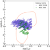 |
Fig. 3 Hertzsprung–Russell diagram for NGC 5128 and NGC 300. The values were calculated using the equations defined in Sect. 3.2. |
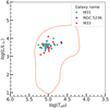 |
Fig. 4 Hertzsprung–Russell diagram for the spiral galaxies. |
3.5 Assessing the accuracy of CSPN parameter estimates
The expressions used to estimate luminosity and temperature (Eqs. (4) and (6)) are affected by several assumptions. In this sense, these determinations are only meaningful in a statistical context involving a significant number of objects, as is the case for NGC 300 and NGC 5128.
The expression used to derive the temperature from the excitation class (Eq. (4)) is an empirical relation. In Reid & Parker (2010b), the authors analyse (considering the uncertainties involved) this temperature determination method and compare it with the Zanstra temperature (see their Fig. 18). In this context, they showed that for optically thick objects, there is a good correlation between the two temperature determinations, while for optically thin objects, the uncertainty exceeds 50%.
Regarding luminosity, the uncertainty depends on the uncertainty in measuring the 5007 Å flux and on the uncertainty in determining the distance to the host galaxy. However, the main source of uncertainty arises from the proportionality constant in Eq. (6). While we can be certain that the uncertainty in this constant is large, assigning it a precise value remains purely speculative (Dopita et al. 1992). For example, if we assume a large uncertainty for the proportionality constant (i.e. 50%), then by propagating the errors we obtain σ(L/L⊙) ≈ 0.7(L/L⊙).
4 Discussion
As can be seen from Figs. 2, 3 and 4, the MW sample of CSPNe is slightly cooler compared to the other galaxies. This difference can be explained by the fact that extragalactic PNe are generally detected through narrowband filters, particularly those centred on [O III]λ5007. Since the ionisation potential for this ion is 35.1 eV, using Eq. (1), we find that only extragalactic CSPNe with temperatures above ≈35 100 K can be detected, corresponding to log(Tef f) > 4.5, which aligns with our findings.
As mentioned in Sect. 3.1, except for the points with temperatures below 35 100 K and the region corresponding to white dwarfs, the physical parameters of CSPNe in the LMC and SMC are distributed within the same region of the HR diagram as those of the MW. This is not the case for NGC 300 and NGC 5128 (Fig. 3), whose objects are concentrated in a more restricted area. In particular, in NGC 300, objects with log(L/L⊙)<2.5 are likely underestimated, as this region corresponds to white dwarfs (see Fig. 9 of Weidmann et al. 2020). In the case of NGC 5128, the clustering of points may be the result of systematic errors in the luminosity estimates, which are likely introduced by the assumptions made during their determination.
Concerning the effective temperature, according to Eq. (4), when the EC exceeds a value of ten, we are likely dealing with objects hotter than 250 × 103 K. This temperature lies at the upper limit of the evolutionary models presented by Miller Bertolami (2016) for stellar masses greater than 0.8 M⊙. Moreover, one of the hottest known stars, WR102, has an effective temperature of 210 kK (see Table 4 of Tramper et al. 2015). In this context, temperatures derived from EC values above ten should be treated with caution.
5 Conclusions
For the first time, the available data on extragalactic CSPNe have been analysed collectively. In addition to compiling information from the literature, physical parameters were computed for over 800 objects. Perhaps the most paradigmatic case is that of the Magellanic Clouds, where, for the first time, the physical parameters of 168 known CSPNe – gathered from 11 different papers – are presented together in an HR diagram. This catalogue constitutes a necessary complement to the catalogue of Galactic CSPNe (Weidmann et al. 2020).
In addition to the effective temperature and luminosity, we have included a handful of CSPNe with determined spectral types that have been reported in the literature. In fact, only 4% of the total sample of 1073 objects have a known spectral type. Moreover, in some cases, only specific spectral features are reported, such as a P-Cygni profile or broad Hα emission. The latter are part of the aforementioned 4%.
Although the spectral types of only a few CSPNe have been accurately determined, it is clear that in the LMC, there are 11 objects with a [WC] central star. Of these, five are classified as [WC 5-8], indicating a relatively high proportion of intermediate subtypes compared to the distribution observed in our Galaxy (Weidmann et al. 2020). While [WC] stars are easier to identify due to their strong emission lines (Werner et al. 2024), previous studies (e.g. Zijlstra et al. 2006, that studied the PNe population of the Sagittarius dwarf spheroidal galaxy) suggest that these spectral types are more frequent in metal-poor environments. Metallicities could also explain the presence of CSPNe of an intermediate subtype rarely found in the MW in the LMC (Monk et al. 1988). In this sense, the SMC, which is more metal poor than the LMC (Table 1), should host a higher proportion of these spectral subtypes. However, only two [WC 5–8] detections have been reported in the SMC out of a total of 47 CSPNe, so no firm conclusions can be drawn given the small number of this sample. However, it is important to reiterate that the compiled catalogue is biased towards brighter stars, and therefore, drawing conclusions about relative population fractions based on metallicity remains highly uncertain.
Objects with high surface temperatures were identified in Magellanic Clouds and NGC 5128. If confirmed to be CSPNe, these sources would represent highly unusual cases due to their potentially high masses, and therefore warrant detailed followup with large telescopes. Such targeted observations could yield valuable data, offering new insights into stellar evolution.
In summary, the catalogue presented here is expected to serve as a valuable resource for guiding future studies, providing a comprehensive and homogeneous compilation of physical parameters for over a thousand CSPNe. It lays the groundwork for targeted spectroscopic follow-up, refined stellar evolution modelling, and comparative analyses across different galactic environments.
Data availability
The catalogue is available at the CDS via https://cdsarc.cds.unistra.fr/viz-bin/cat/J/A+A/701/A125
Acknowledgements
We are grateful to the anonymous referee for their valuable feedback, which greatly enhanced this manuscript. WW thanks Luis Gutiérrez-Soto for his support. This work was partially supported by grants PICT 2021-00442 awarded by Foncyt, grant PIP 2022 11220210100520CO by CONICET, and by grant SeCyT UNC Consolidar project 2023 NRO: 33620230100103CB. This research has made use of NASA’s Astrophysics Data System Service. This research has made use of the SIMBAD database, operated at CDS, Strasbourg, France.
References
- Acker, A., Jasniewicz, G., Koeppen, J., & Stenholm, B. 1989, A&AS, 80, 201 [Google Scholar]
- Appleton, P. N., Davies, R. D., & Stephenson, R. J. 1981, MNRAS, 195, 327 [NASA ADS] [CrossRef] [Google Scholar]
- Arnaboldi, M., Gerhard, O., Okamura, S., et al. 2007, PASJ, 59, 419 [NASA ADS] [Google Scholar]
- Beasley, M. A., Fahrion, K., & Gvozdenko, A. 2024, MNRAS, 527, 5767 [Google Scholar]
- Choudhury, S., de Grijs, R., Rubele, S., et al. 2020, MNRAS, 497, 3746 [NASA ADS] [CrossRef] [Google Scholar]
- Ciardullo, R., Jacoby, G. H., Ford, H. C., & Neill, J. D. 1989, ApJ, 339, 53 [Google Scholar]
- Ciardullo, R., Durrell, P. R., Laychak, M. B., et al. 2004, ApJ, 614, 167 [Google Scholar]
- Ciardullo, R., Sigurdsson, S., Feldmeier, J. J., & Jacoby, G. H. 2005, ApJ, 629, 499 [Google Scholar]
- de Vaucouleurs, G., de Vaucouleurs, A., Corwin, Herold G., J., et al. 1991, Third Reference Catalogue of Bright Galaxies (New York, USA: Springer) [Google Scholar]
- Delgado-Inglada, G., García-Rojas, J., Stasińska, G., & Rechy-García, J. S. 2020, MNRAS, 498, 5367 [NASA ADS] [CrossRef] [Google Scholar]
- Dopita, M. A., & Meatheringham, S. J. 1991a, ApJ, 367, 115 [Google Scholar]
- Dopita, M. A., & Meatheringham, S. J. 1991b, ApJ, 377, 480 [Google Scholar]
- Dopita, M. A., Jacoby, G. H., & Vassiliadis, E. 1992, ApJ, 389, 27 [Google Scholar]
- Dopita, M. A., Vassiliadis, E., Wood, P. R., et al. 1997, ApJ, 474, 188 [NASA ADS] [CrossRef] [Google Scholar]
- Ferland, G. J., Korista, K. T., Verner, D. A., et al. 1998, PASP, 110, 761 [Google Scholar]
- Flores-Durán, S. N., Peña, M., & Ruiz, M. T. 2017, A&A, 601, A147 [NASA ADS] [CrossRef] [EDP Sciences] [Google Scholar]
- Ford, H., Peng, E., & Freeman, K. 2002, in The Dynamics, Structure & History of Galaxies: A Workshop in Honour of Professor Ken Freeman, eds. G. S. Da Costa, E. M. Sadler, & H. Jerjen, Astronomical Society of the Pacific Conference Series, 273, 41 [Google Scholar]
- Freedman, W. L., Madore, B. F., Gibson, B. K., et al. 2001, ApJ, 553, 47 [Google Scholar]
- Frew, D. J., & Parker, Q. A. 2010, PASA, 27, 129 [CrossRef] [Google Scholar]
- Geha, M., van der Marel, R. P., Guhathakurta, P., et al. 2010, ApJ, 711, 361 [NASA ADS] [CrossRef] [Google Scholar]
- Gesicki, K., Zijlstra, A. A., & Miller Bertolami, M. M. 2018, Nat. Astron., 2, 580 [NASA ADS] [CrossRef] [Google Scholar]
- González-Santamaría, I., Manteiga, M., Manchado, A., et al. 2021, A&A, 656, A51 [NASA ADS] [CrossRef] [EDP Sciences] [Google Scholar]
- Harris, J., & Zaritsky, D. 2009, AJ, 138, 1243 [NASA ADS] [CrossRef] [Google Scholar]
- Herald, J. E., & Bianchi, L. 2004, ApJ, 611, 294 [NASA ADS] [CrossRef] [Google Scholar]
- Hui, X., Ford, H. C., Ciardullo, R., & Jacoby, G. H. 1993, ApJS, 88, 423 [Google Scholar]
- Jacoby, G. H. 1989, ApJ, 339, 39 [NASA ADS] [CrossRef] [Google Scholar]
- Jacoby, G. H., & Ciardullo, R. 1999, ApJ, 515, 169 [CrossRef] [Google Scholar]
- Kwitter, K. B., & Henry, R. B. C. 2022, PASP, 134, 022001 [NASA ADS] [CrossRef] [Google Scholar]
- Kwok, S. 2007, The Origin and Evolution of Planetary Nebulae (Cambridge, UK: Cambridge University Press) [Google Scholar]
- Licquia, T. C., & Newman, J. A. 2015, ApJ, 806, 96 [NASA ADS] [CrossRef] [Google Scholar]
- Magrini, L. 2006, in Planetary Nebulae in our Galaxy and Beyond, eds. M. J. Barlow, & R. H. Méndez, IAU Symposium, 234, 9 [Google Scholar]
- Mateo, M. L. 1998, ARA&A, 36, 435 [NASA ADS] [CrossRef] [Google Scholar]
- Mazzi, A., Girardi, L., Zaggia, S., et al. 2021, MNRAS, 508, 245 [NASA ADS] [CrossRef] [Google Scholar]
- McConnachie, A. W. 2012, AJ, 144, 4 [Google Scholar]
- Mendez, R. H., Kudritzki, R. P., Herrero, A., Husfeld, D., & Groth, H. G. 1988, A&A, 190, 113 [NASA ADS] [Google Scholar]
- Merrett, H. R., Merrifield, M. R., Douglas, N. G., et al. 2006, MNRAS, 369, 120 [NASA ADS] [CrossRef] [Google Scholar]
- Miller Bertolami, M. M. 2016, A&A, 588, A25 [NASA ADS] [CrossRef] [EDP Sciences] [Google Scholar]
- Monk, D. J., Barlow, M. J., & Clegg, R. E. S. 1988, MNRAS, 234, 583 [NASA ADS] [CrossRef] [Google Scholar]
- Murset, U., & Nussbaumer, H. 1994, A&A, 282, 586 [Google Scholar]
- Ostlie, D. A., & Carroll, B. W. 1996, An Introduction to Modern Stellar Astrophysics [Google Scholar]
- Reid, W. A., & Parker, Q. A. 2010a, MNRAS, 405, 1349 [Google Scholar]
- Reid, W. A., & Parker, Q. A. 2010b, PASA, 27, 187 [Google Scholar]
- Richer, M. G., & McCall, M. L. 2008, ApJ, 684, 1190 [Google Scholar]
- Richer, H. B., Pritchet, C. J., & Crabtree, D. R. 1985, ApJ, 298, 240 [Google Scholar]
- Rolleston, W. R. J., Trundle, C., & Dufton, P. L. 2002, A&A, 396, 53 [NASA ADS] [CrossRef] [EDP Sciences] [Google Scholar]
- Schönberner, D., Jacob, R., Sandin, C., & Steffen, M. 2010, A&A, 523, A86 [NASA ADS] [CrossRef] [EDP Sciences] [Google Scholar]
- Shenar, T. 2024, arXiv e-prints [arXiv:2410.04436] [Google Scholar]
- Soemitro, A. A., Roth, M. M., Weilbacher, P. M., et al. 2023, A&A, 671, A142 [NASA ADS] [CrossRef] [EDP Sciences] [Google Scholar]
- Spiniello, C., Napolitano, N. R., Arnaboldi, M., et al. 2018, MNRAS, 477, 1880 [Google Scholar]
- Stanghellini, L., & Haywood, M. 2010, ApJ, 714, 1096 [NASA ADS] [CrossRef] [Google Scholar]
- Stanghellini, L., Magrini, L., Villaver, E., & Galli, D. 2010, A&A, 521, A3 [NASA ADS] [CrossRef] [EDP Sciences] [Google Scholar]
- Tramper, F., Straal, S. M., Sanyal, D., et al. 2015, A&A, 581, A110 [NASA ADS] [CrossRef] [EDP Sciences] [Google Scholar]
- Valenzuela, L. M., Miller Bertolami, M. M., Remus, R.-S., & Méndez, R. H. 2025, A&A 699, A371 [NASA ADS] [CrossRef] [EDP Sciences] [Google Scholar]
- Villaver, E., Stanghellini, L., & Shaw, R. A. 2004, ApJ, 614, 716 [Google Scholar]
- Villaver, E., Stanghellini, L., & Shaw, R. A. 2007, ApJ, 656, 831 [NASA ADS] [CrossRef] [Google Scholar]
- Walsh, J. R., Rejkuba, M., & Walton, N. A. 2015, A&A, 574, A109 [NASA ADS] [CrossRef] [EDP Sciences] [Google Scholar]
- Weidmann, W. A., & Gamen, R. 2011, A&A, 526, A6 [NASA ADS] [CrossRef] [EDP Sciences] [Google Scholar]
- Weidmann, W. A., Mari, M. B., Schmidt, E. O., et al. 2020, A&A, 640, A10 [NASA ADS] [CrossRef] [EDP Sciences] [Google Scholar]
- Werner, K., Todt, H., Bond, H. E., & Zeimann, G. R. 2024, A&A, 686, A29 [NASA ADS] [CrossRef] [EDP Sciences] [Google Scholar]
- Zijlstra, A. A., Gesicki, K., Walsh, J. R., et al. 2006, MNRAS, 369, 875 [NASA ADS] [CrossRef] [Google Scholar]
All Tables
Main parameters of the galaxies in our sample. Namely, these are galaxy name, number of catalogued PNe, metallicity, morphological type, color, and global stellar mass.
All Figures
|
Fig. 1 Hertzsprung–Russell diagram showing CSPNe within the MW from Weidmann et al. (2020). The marginal curves represent the data using a continuous probability density curve. |
| In the text | |
|
Fig. 2 Hertzsprung–Russell diagram of CSPNe in the LMC and SMC. The coldest CSPN in the SMC likely has poorly constrained parameters, as an effective temperature (Teff) above 10 000 K is required to efficiently ionise hydrogen. The orange contour shows the distribution of points for the MW. In grey, two regions with extreme values are highlighted (see text for details). |
| In the text | |
|
Fig. 3 Hertzsprung–Russell diagram for NGC 5128 and NGC 300. The values were calculated using the equations defined in Sect. 3.2. |
| In the text | |
|
Fig. 4 Hertzsprung–Russell diagram for the spiral galaxies. |
| In the text | |
Current usage metrics show cumulative count of Article Views (full-text article views including HTML views, PDF and ePub downloads, according to the available data) and Abstracts Views on Vision4Press platform.
Data correspond to usage on the plateform after 2015. The current usage metrics is available 48-96 hours after online publication and is updated daily on week days.
Initial download of the metrics may take a while.