| Issue |
A&A
Volume 702, October 2025
|
|
|---|---|---|
| Article Number | A159 | |
| Number of page(s) | 10 | |
| Section | Astronomical instrumentation | |
| DOI | https://doi.org/10.1051/0004-6361/202452515 | |
| Published online | 16 October 2025 | |
Adaptive uniform weighting: Pre-conditioning to improve image fidelity
SKA Observatory,
Jodrell Bank,
SK11 9FT,
UK
★ Corresponding author: This email address is being protected from spambots. You need JavaScript enabled to view it.
Received:
7
October
2024
Accepted:
6
August
2025
Abstract
Context. The ‘dirty image’ produced as a result of a direct Fourier inversion of visibility data is an important first step in inteferometric imaging. This is where we define the ‘deconvolution problem’, and the extent to which that problem is well- or ill-conditioned has direct consequences for the ultimate image fidelity that can be achieved in practise.
Aims. An under-utilised degree of freedom during Fourier imaging pertains to the relative weights that are assigned to the visibility data. We explore the circumstances where some adjustment of the relative weights could provide improvements to the dirty image and, consequently, the ultimate post-deconvolution image fidelity.
Methods. In this work, we specifically explored whether typical observations with current and upcoming facilities demonstrate a significant radial trend in the acquired data density. We modelled those trends and used them to calculate a distinct effective local density estimate for each data point.
Results. When the resulting local density estimate is used in conjunction with a uniform weight correction and the desired clean beam (e.g. Gaussian) tapering, it provides a significant improvement in the image quality over that provided by the current pixel-based density estimate. This distinction disappears in cases where the acquired visibility sampling is essentially complete.
Conclusions. In many cases, particularly spectral-line observations (especially those with only limited sidereal tracking), this adaptive approach improves the beam quality by a factor of 2–10, as measured by the RMS residual relative to the best-fitting clean beam. This results in an improvement in the final image fidelity that is similar in terms of magnitude. An appealing aspect of this approach is that there are no ‘knobs’ for the user to adjust. Once the field size and pixel size are specified (guided by astrophysical aims), the method is considered to be fully adaptive to the acquired data and produces the ‘cleanest possible’ dirty beam in these circumstances.
Key words: techniques: high angular resolution / techniques: image processing / techniques: interferometric
© The Authors 2025
 Open Access article, published by EDP Sciences, under the terms of the Creative Commons Attribution License (https://creativecommons.org/licenses/by/4.0), which permits unrestricted use, distribution, and reproduction in any medium, provided the original work is properly cited.
This article is published in open access under the Subscribe to Open model. This email address is being protected from spambots. You need JavaScript enabled to view it. to support open access publication.
1 Introduction
Interferometric imaging in radio astronomy Thompson et al. (2017) has been utilised for more than six decades as a means of achieving higher angular resolution than is currently possible with monolithic single dish radio telescopes. Although the basic principles are well-understood, there are still areas where the practical implementation of those principles could benefit from further analysis. One aspect in particular that we consider here is the choice of data weighting that is applied to the measured visibilities. Despite its importance in determining image properties, such as thermal noise, source confusion, and image fidelity, this area has been rather poorly studied. One reason for this lack of interest in optimising the data weighting might be that it is considered only of marginal relevance since it applies to the so-called dirty interferometric image, which must inevitably be deconvolved to achieve a ‘clean’ outcome prior to any quantitative analysis. In fact, it is actually of fundamental importance to achieve the ‘cleanest possible dirty image’ via linear means during the imaging process itself. In this way, the image flux scale is best preserved by matching beams of any modelled emission with the inevitably unmodelled image residuals. And perhaps of even greater importance is the issue of image fidelity. As we demonstrate in this work, the cleanest possible dirty beam produced by only linear means provides quite a good indication of the intrinsic image fidelity; namely, the normalised difference between intrinsic and reconstructed image structures after deconvolution. Once non-linear methods are introduced into the imaging problem, they bring on their inherent biases and assumptions about the underlying sky brightness, which have been designed to make images that are plausible in terms of appearance, but are often not reproducible when higher resolution and sensitivity observations become available.
2 The imaging problem
The challenge we face in interferometric imaging is estimation of a robust, high-fidelity gridded representation of the sky brightness, using incomplete and noisy measurements of its Fourier transform that is suitable for quantitative analysis. Since the field of view is often large relative to the angular resolution, it can encompass >106 distinct sources above the noise floor, all of an a priori unknown detailed morphology. This makes it vital for the resulting clean image to have a well-defined, position-invariant PSF that can be unambiguously represented on both the imaging grid, and (ideally) its Fourier transform, particularly for sources that will inevitably not be centered on image pixels. For a given pixel size, δ, an obvious choice for the clean PSF is a Gaussian with FWHM ≳2.5δ. Other functional forms might also be considered for the clean PSF if they satisfy these requirements and brought additional benefits.
3 Data weighting
When considering the impact of visibility data weighting on the PSF, we only need consider the small angle approximation, where the line-of-sight w coordinate of projected baseline length is ignored, since the three dimensional (3D) treatment is only required to make the bore-sight PSF invariant across the field, as we explicitly verify below. As outlined in Thompson et al. (2017), the measured visibility data, Vmeas(u, v), can be related to the intrinsic visibility data, V(u, v), as
 (1)
(1)
where W(u, v) represents the transfer function that expresses the visibility sampling achieved by the instantaneous interferometric array configuration in conjunction with any sidereal tracking. Data weighting refers to the term, w(u, v), in the equation above. The measured dirty image is given by the Fourier transform of that equation,
 (2)
(2)
where the asterisk, *, represents a 2D convolution and b0(l, m) is the dirty beam, which is the Fourier transform of W(u, v) w(u, v). Historically, there have only been two basic data weighting methods used, deemed ‘natural’ and ‘uniform’. Natural (NA) weighting makes use of the inverse data variance for w(u, v) and results in images with the lowest possible receiver noise fluctuation level, although often at the expense of very undesirable dirty beam properties for typical array configurations. In fact, in many circumstances, the natural PSF can have both extremely broad side-lobes that scatter even compact source power out to large angular distances as well as a central cusp that is under-sampled relative to the imaging grid. This creates an ill-conditioned imaging problem. On the other hand, uniform (UW) weighting makes use of the inverse data density,
 (3)
(3)
most often in conjunction with a tapering function wt(u, v), that represents the form of a clean ‘restoring’ beam, so that we have
 (4)
(4)
where the tapering is normally chosen to be a Gaussian, due to its many desirable properties, as noted in the previous section. The most useful Gaussian tapers are those that satisfy the Nyquist-Shannon sampling theorem (corresponding to an image plane PSF with FWHM ≳ 2.5δ) and decline to small values at the largest radii where data have been acquired, so that an extrapolation to larger radii (by non-linear deconvolution methods) is not necessary.
A third weighting option was developed by Briggs (1995) in which a tunable ‘robustness’ parameter allows the user to choose some linear combination of natural and uniform weighting factors to yield beam and noise properties that are intermediate between the two methods. This approach provides very little control of the resulting dirty PSF shape and could also lead to a PSF that is not fully sampled on the imaging grid.
A final variant that has been implemented in some imaging software is known as ‘super-uniform’ weighting. In this case, the inverse data density factor is evaluated on a coarser grid than that used for imaging, typically an integer multiple of the original pixel size. Although this can sometimes be beneficial, there are also some potential pitfalls with this approach, as we discuss below.
We provide some motivation for exploring alternative data weighting approaches by contrasting the image fidelity of restored deconvolved images resulting from dirty images made with NA, Briggs (BRI, using miriad robust = 0), and UW weighting, as well as the adaptive uniform weighting (AUW) strategy defined here for a monochromatic, four-hour tracking observation with SKA-Low in Fig. 1. We explored a wide range of signal-to-noise ratio (S/N) scenarios, including noise-free, low-noise (nominal/3), nominal noise, and high-noise (nominal×5). Image fidelity is defined here as
 (5)
(5)
where the magnitude of the Fourier transform, ℱ, of the difference between the ideal sky model, S, and the restored sky model, R, is normalised by the ideal sky model magnitude. The image fidelity has been averaged in logarithmically spaced annuli to demonstrate its variation with scale. The sky model, imaging, and deconvolution simulations are described in Appendix A and the sky model itself is shown in Fig. 2. What is apparent from Fig. 1 is that the resulting image fidelity is closely tied to the quality of the dirty image, that is, the degree to which the dirty PSF is already consistent with the ultimately desired restoring function for the image. The only circumstance to which this does not apply is when the S/N is so low that the source detection (rather than a quantitative characterisation) is the aim. As expected, natural weighting is unsurpassed for source detection, but poorly suited to a complex source characterisation.
4 Data density
A vital quantity that underlies the uniform weighting strategy is the data density, ρ(u, v). While conceptually simple, this quantity can only be specified analytically in a few special cases, such as a linear, regularly sampled, east-west array undertaking a full 12-hour tracking observation at high declination (Thompson et al. 2017) for which ρ(u, v) ∝ 1/(u2 + v2)1/2. For a more typical array configuration and track duration, the estimation of local data density becomes much more problematic.
The most common implementation of data density estimation makes use of the data grid that is defined for Fourier transform imaging. Prior to the actual data gridding step, which involves convolution to a grid with a suitable gridding kernel (while potentially taking explicit account of the w coordinate), the weights applied to the data are first determined in only the (u, v) plane. A simple sum of data points that fall (in the nearest pixel sense) within each (u, v) cell provides the local density estimate. In the event that the majority of (u, v) cells contain at least one data point, this is an excellent estimate. However, this condition is rarely met in practise. If we consider imaging with a relatively fine pixel sampling and only short observation duration, then we can often approach the regime where each (u, v) cell has only either a single data value or none at all, while the overall fraction of filled cells is rather low. In this case, there is little distinction between natural and uniform weighting, and all of the resulting dirty beams are equally bad.
5 Adaptive uniform weighting
We explored an alternative strategy for local density estimation for use in a uniform weighting correction. In doing so, we made a clear distinction between a factor needed to account for multiple measurements within the same cell, wm(u, v), and the factor needed to account for the local density of occupied cells, wo(u, v). The uniform weight correction factor is the product of the two,
 (6)
(6)
We started by forming the gridded distributions of data multiplicity, M(u, v), and data occupancy, O(u, v), while also determining the minimum and maximum radii, rmin and rmax (in units of pixels), where data occur. It is important to note that while the multiplicity distribution can have values of either 0 or any positive integer, the occupancy distribution has only values of either 0 or 1. Next, we considered whether there might be any systematic variation of the average occupation density as function of radius in the visibility plane, o(r). There are at least two reasons why such a trend might be present. Firstly, many array configurations tend to be centrally concentrated to provide high surface brightness sensitivity, so that there is often a radial decline in the number of sampled (u, v) points. Secondly, as noted in the previous section, the presence of any sidereal tracking also gives rise to a natural radial decline in the data occupancy.
We considered the distributions of o(r) for many array configurations of current facilities: ALMA (Cortes et al. 2024), LOFAR (van Haarlem et al. 2013), MeerKAT (Jonas 2009), and VLA (Napier et al. 1983), as well as the upcoming SKA-Low and SKA-Mid (Braun et al. 2019). What we find is a wide variety of behaviours, which can be summarised as follows. There is a peak occupancy, op, at some value of r = rp and there is a possible roll-off of average occupancy both to larger and in some cases smaller radii. Some examples of average occupancy are provided below in Appendix B.
The strategy we explored here is adaptive to the local average occupancy. For radii with an average occupancy that is greater than a certain cut-off value, o(r) ≥ ot, we simply adopted the standard UW approach, where the local occupancy is equal to the gridded occupancy,
 (7)
(7)
Meanwhile, for radii where o(r) < ot, we undertook an alternate local occupancy density estimation. This was accomplished by using the average occupancy at each radius to define a smoothing kernel diameter,
 (8)
(8)
which is a factor of T larger than what yields an average of one occupied cell per kernel. Each occupied cell of O(u, v) is convolved with the smoothing kernel, k(u, v), chosen for example to be a uniform disk with diameter, d(r), and normalised to an integral of unity,
 (9)
(9)
This is the local occupation density estimator that provides wo(u, v) = 1/o(u, v) to be used in conjunction with the multiplicity factor wm(u, v) = 1/M(u, v) in Equation (6). We explored alternate smoothing kernel definitions, but found no benefit in using more complex kernel shapes.
We note that the variable, T, was introduced in Equation (8) to ensure that the smoothing kernel spans multiple occupied cells. This is necessary to accommodate potential variability in the occupation density with azimuthal angle at each radius. It was found that a value T ~ 3 seems to perform best in terms of the resulting dirty beam quality.
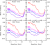 |
Fig. 1 Comparison of restored image fidelity with standard UW, BRI, NA, and AUW for a noise-less (top-left), low-noise (top-right), nominal-noise (bottom-left), and high-noise (bottom-right) monochromatic 4-hour tracking observation with SKA-Low. The image fidelity has been averaged in logarithmically spaced annuli. |
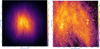 |
Fig. 2 Sky model used for image fidelity simulations. The full 6.4 × 6.4 degree field tapered with the primary beam model is shown on the left and the central portion on the right. The peak brightness is 1.5 Jy/Beam, the diffuse emission plateau has brightness of 0.2 mJy/Beam (about 25 K), and the faintest discrete sources are <1 µJy/Beam. |
6 Relative PSF performance
We implemented the AUW method, using the detailed implementation outlined in Appendix B, within the miriad package (Sault et al. 1995) imaging task invert to explore its utility. We then contrasted its performance with the standard pixel-based density estimator of the UW approach. We made use of the SKA-Mid and SKA-Low Design Baseline array configurations, as well as those of MeerKAT, the VLA-A configuration, LOFAR, and ALMA (in its Cycle 10-8 configuration). We explored both transit snap-shot and sidereal track (for Dec = −/+ 30° and -4h < HA < +4h for the mid-frequency dish arrays and −2h < HA < +2h tracks for aperture arrays and ALMA) imaging for both monochromatic and multi-frequency synthesis (MFS with Δν/ν = 0.4) continuum observations. For the sidereal tracking simulations we adopt a sampling interval of 1 minute, rather than the shorter time interval that would represent continuous data acquisition at a rate which minimises time smearing. This is done to keep the simulation times and data quantities more tractable.
For each simulated observation, we explored the full range of angular scales that the array configuration provides, by defining a logarithmic sequence of target Gaussian FWHM beams, θt, that define the Gaussian tapering function, wt(u, v), at an arbitrary reference frequency accessible to that array. The pixel size was chosen to be θt / 4 and the image size is chosen to ideally span a diameter of 1.5× the first null of the primary beam pattern (although it is also constrained to be in the range 1024 ≤ Npix ≤ 16 384 pixels).
We illustrate the relative PSF properties of AUW versus standard UW in Figure 3 for SKA-Mid. For the standard UW results we have undertaken the same imaging simulations with both miriad (Sault et al. 1995) as well as wsclean (Offringa et al. 2014). While both produce similar results, the wsclean images demonstrate a more robust continuity with imaging parameters and are used for all of the comparisons below.
The SKA-Mid array configuration provides good sensitivity, as measured by the ratio of RMS image noise relative to the NA image noise, to an extremely wide range of angular scales (about 1000:1) as can be seen in the bottom panels. The quality of the dirty PSF, Q, is measured by the RMS residual within the central 16 × 16 beam FWHM after subtracting the best-fitting Gaussian, and is shown in the other panels of the figure. Not surprisingly, a better PSF quality is achieved in sidereal tracking observations relative to snap-shots, as well as MFS observations relative to monochromatic ones. In those cases where the visibility sampling is already essentially complete, there is no distinction between the UW and AUW PSF. The distinction becomes apparent when higher angular resolution is targeted, in this case below about 10 arcsec (at a reference frequency of 1.4 GHz) and is largest for the monochromatic and snap-shot coverage cases, where there can be up to an order of magnitude lower PSF RMS. The more Gaussian PSF provided by AUW imaging is also accompanied by more effective tracking of the target Gaussian FWHM in each simulation, extending the highest angular resolution achievable by a factor of about 1.5, up to the diffraction limit of the array. The improved and more compact PSF, particularly for the monochromatic case, does come at the expense of a somewhat enhanced RMS image noise (as seen in the lower left panel of the figure).
The same AUW versus UW comparison is shown in Figures C.1 (LOFAR), C.2 (SKA-Low), C.3 (MeerKAT), C.4 (VLA), and C.5 (ALMA). Very similar trends to those already noted for SKA-Mid can be seen in these cases. The most significant improvements in PSF quality are obtained for monochromatic observations as well as for less complete sidereal tracking.
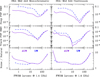 |
Fig. 3 Comparison of imaging performance with standard UW (dashed lines) and AUW (solid lines) for SKA-Mid. The monochromatic case is on the left and multi-frequency synthesis with 40% fractional bandwidth on the right. Bottom panels show the image RMS noise relative to NA weighting. The other panels show the RMS residual after a Gaussian fit to the PSF for a snap-shot (top) and full track (centre) observation. |
7 Discussion
7.1 Benefits
As noted in Sect. 3 and illustrated in Fig. 1, the primary motivation for improving the quality of the dirty PSF comes from enhancing the image fidelity that will ultimately be achieved following any required deconvolution. It is apparent from Fig. 1 that we have significant improvement in the final image fidelity over the complete range of angular scales provided by the array configuration that scales with the quality of the dirty PSF. This generalisation only breaks down in the noise-dominated regime, where the higher RMS noise that accompanies an improved dirty PSF begins to limit source detectability relative to the more ’natural’ visibility weightings. To put this series of simulations into context (a monochromatic 4h tracking observation with SKA-Low) it is useful to consider the left-hand-central panel of Fig. C.2. The PSF RMS for the AUW and UW cases is about Q = 0.01 and 0.03 respectively for a target FWHM near 10 arcsec. This is comparable to the best noise-free image fidelity, F, that is achieved at intermediate angular scales for these two weighting methods in our simulations. As the image S/N level decreases, the image fidelity deteriorates from this starting point. This sequence of simulations demonstrates that the dirty PSF RMS, Q provides a plausible best-case (high S/N, negligible calibration error) estimate of the final deconvolved image fidelity, F. It is clearly very desirable to achieve the cleanest possible dirty image.
7.2 Optimisation
The specific implementation of the AUW strategy described in Appendix B has been shown to be moderately effective in Figures 3, C.1, C.2, C.3, C.4 and C.5. However, there is undoubtedly scope for further optimisation of this approach. We have employed a discrete convolution to obtain a local estimate of occupation density at radii where the azimuthally averaged density declines below unity. While this has an acceptable computational cost for moderate visibility numbers, it may be more efficiently undertaken with a sequence of FFT-based convolutions using Gaussian tapers that sample the required range of (u, v) kernel sizes.
Another indication that further optimisation is needed comes from the occasionally discontinuous behaviour of the resulting PSF properties with the gridding parameters. A noteworthy case is the full-track MeerKAT MFS case shown in Figure C.3, where the PSF RMS demonstrates some oscillatory behaviour when targeting FWHM in the range 4–20 arcsec.
7.3 Relation to super-uniform weighting
It is worth noting that the occurrence of an average data occupancy of less than unity is exactly what motivates the use of ’super-uniform’ weighting. However, while the adaptive approach attempts to track the spatial variation of occupancy density, the super-uniform method employs a single, typically square smoothing kernel for the entire visibility grid. In this context, it is also worth drawing attention to the fact that those implementations of super-uniform weighting, which simply employ a coarser super-grid that consolidates n × n original (u, v) pixels into one, are prone to generate aliased secondary peaks in the PSF at multiples of 1/n of the field size in both dimensions. A robust implementation of super-uniform weighting would involve the gridded weights being subject instead to convolution with an appropriate kernel; for example, a Gaussian with FWHM of several (u, v) cells. This robust method of super-uniform weighting has been implemented within the miriad package as the radfft option within the invert imaging task.
7.4 Application to the full 3D imaging case
As noted at the outset, the strategy outlined here for visibility weight determination has deliberately considered the case where the w coordinate of the visibility data can be ignored. For wide-field imaging at relatively low radio frequencies, this is rarely the case. However, once the visibility weights have been determined for an optimised bore-sight PSF, as outlined in this manuscript, they can be used in conjunction with any desired 3D imaging technique, such as w-projection (Cornwell et al. 2005) or w-stacking Offringa et al. (2014) to achieve the necessary degree of position invariance of the PSF across the field. We tested this assertion explicitly, by implementing the algorithm described in Appendix B as a stand-alone python script that provides pre-processing of a visibility database and produces a ‘Measure-mentSet’ (MS) that can be imaged and deconvolved with other applications. The visibility data weights were optimised for a specific desired image (in terms of field size, pixel sampling, and possible multi-frequency synthesis). The MS was then imaged with wsclean by specifying a natural weighting together with a Gaussian tapering appropriate for the image pixel size. This approach exhibited an accurate field invariance (as specified by the wgridder-accuracy parameter) of the bore-sight PSF, along with its excellent AUW attributes.
Acknowledgements
The assistance and support of Mark Wieringa during the implementation of this strategy into the miriad package invert task as the weighting option “radial” is greatly appreciated, as is his implementation of an FFT-based “super-uniform” weighting option “radfft” within invert.
References
- Bonaldi, A., Hartley, P., Ronconi, T., De Zotti, G., & Bonato, M. 2023, MNRAS, 524, 993 [CrossRef] [Google Scholar]
- Bracco, A., Ntormousi, E., Jelic, V., et al. 2022, A&A, 663, A37 [NASA ADS] [CrossRef] [EDP Sciences] [Google Scholar]
- Braun, R., Bonaldi, A., Bourke, T., et al. 2019, arXiv e-prints [arXiv:1912.12699] [Google Scholar]
- Briggs, D. S., High Fidelity Deconvolution of Moderately Resolved Sources, Ph.D. thesis, New Mexico Institute of Mining and Technology (1995), Mexico [Google Scholar]
- Cornwell, T. J., Golap, K. & Bhatnagar, S. 2005, Astronomical Data Analysis Software and Systems XIV, 347, 86 [Google Scholar]
- Cortes, P. C., Vlahakis, C., Hales, A., et al. 2024, ALMA Technical Handbook, ALMA Doc. 11.3, Ver. 1.4 [Google Scholar]
- Jonas, J. L. 2009, IEEE Proceedings, 97, 1522 [NASA ADS] [CrossRef] [Google Scholar]
- Lynch, C. R., Galvin, T. J., Line, J. L. B., et al. 2021, Publ. Astron. Soc. Australia, 38, e057 [Google Scholar]
- Napier, P. J., Thompson, A. R., & Ekers, R. D. 1983, IEEE Proceedings, 71, 1295 [CrossRef] [Google Scholar]
- Offringa, A. R., McKinley, B., Hurley-Walker, N., et al. 2014, MNRAS, 444, 606 [Google Scholar]
- Sault, R. J., Teuben, P. J., & Wright, M. C. H. 1995, Astronomical Data Analysis Software and Systems IV, 77, 433 [Google Scholar]
- Thompson, A. R., Moran, J. M., & Swenson, G. W. 2017, Interferometry and Synthesis in Radio Astronomy, 3rd edn., eds. A. R. Thompson, J. M. Moran, & G. W. Swenson, Jr. (Berlin: Springer) [Google Scholar]
- van Haarlem, M. P., Wise, M. W., Gunst, A. W., et al. 2013, A&A, 556, A2 [NASA ADS] [CrossRef] [EDP Sciences] [Google Scholar]
Appendix A Image fidelity simulations
Here, we describe the imaging and deconvolution simulations undertaken to quantify image fidelity. We constructed a realistic sky model, S, for relatively low radio frequencies (180 MHz as an example) and Southern declinations at relatively high Galactic latitude by beginning with the GLEAM survey (Lynch et al. 2021) complete to 100 mJy and supplementing this with a T-RECs simulation (Bonaldi et al. 2023) with a statistically accurate representation of extragalactic source numbers and morphologies between 100 mJy and 1 µJy (about 1.5 × 10⁷ in number). A plausible diffuse Galactic foreground for the field was drawn from an MHD simulation of the ISM (Bracco et al. 2022) and this was arbitrarily assigned a peak brightness of about 25 K, consistent with expectations for a high latitude field. The complete model spanning 6.4 degree, was gridded with a 12.5 arcsec FWHM circular Gaussian on a 4 arcsec grid and spatially tapered with a model of the primary beam, including its first side-lobe, prior to being zero-padded to double the pixel number in both dimensions (11520 × 11520). The resulting sky model is shown in Fig. 2
Dirty beams, b, and noise images, N, were generated from a simulated monochromatic 180 MHz observation with miriad uvgen spanning hour angles of −2h to +2h, sampled at intervals of 15m for the SKA-Low configuration of 512 stations with Bmax ~ 74km. miriad invert was used to produce the dirty beams with NA, BRI (robust = 0), UW, and AUW (options = radial) sampled by (11520 × 11520) pixels of 4 arcsec. The BRI, UW, and AUW beams were generated with a Gaussian taper of 12.5 arcsec FWHM, while the NA beam was left untapered.
A deconvolved sky model representation, S′, was generated from the (11520 × 11520) Gaussian gridded model by a linear deconvolution of a unit height 12.5 arcsec FWHM Gaussian, G, truncated at 1 × 10⁻⁶,
 (A.1)
(A.1)
Convolved dirty images, D, were constructed as
 (A.2)
(A.2)
The dirty images and beams were used to undertake a deconvolution of the field with miriad clean. All deconvolved models were restored with a 12.5 arcsec FWHM Gaussian that was added to the relevant residuals. The deconvolution was undertaken both in the absence of noise, and with low-, nominal- and high-noise values; Natural RMS noise of σNA = 0, 41, 124, 620 µJy/Beam. The corresponding RMS noise values for the BRI, UW, and AUW cases are higher than the NA values by factors of 1.35, 1.67, and 2.41 respectively in all cases. For most cases (noise-free, low- and nominal-noise), a target brightness limit of 1 × 10⁻⁴ Jy/beam or iteration number limit of 106 was specified. For the high-noise case a target brightness limit of 5 × 10⁻⁴ Jy/beam or iteration number limit of 2 × 10⁵ was specified. The BRI, UW and AUW images were all able to reach the requested brightness limit, although this required fewer iterations with UW and fewer still for AUW. The NA weighted decon-volutions made little net progress and terminated after the full iteration number without reaching the target brightness limits in any of the cases considered.
Appendix B Implementation strategy
Here we outline the specific implementation of the AUW strategy within the miriad (Sault et al. 1995) package imaging task invert.
As noted in Sect. 3, the gridded distributions of data multiplicity M(u, v) and occupancy O(u, v) are first accumulated on the basis of data assignment to only the nearest pixel in the grid. At the same time the minimum and maximum radii, rmin and rmax, (in units of pixels) where data occur are also determined, while imposing the constraint that rmax < Npix/2. This is done to preserve circular symmetry in the resulting beam shape.
We then define a set of radial annuli with a logarithmic radial step. We arbitrarily choose a number of bins nr = (rmax – rmin)1/2, constrained to be nr ≤ 64 that define a set of outer radii, ri given by,
![Mathematical equation: ${r_i} = antilo{g_{10}}\left[ {lo{g_{10}}\left( {{r_{min}}} \right) + i \times lo{g_{10}}\left( {{r_0}} \right)} \right],\,\,i = 1, \ldots {n_r},$](/articles/aa/full_html/2025/10/aa52515-24/aa52515-24-eq12.png) (B.1)
(B.1)
where
![Mathematical equation: ${r_0} = antilo{g_{10}}\left[ {lo{g_{10}}\left( {{r_{max}}} \right) - lo{g_{10}}\left( {{r_{min}}} \right))/{n_r}} \right].$](/articles/aa/full_html/2025/10/aa52515-24/aa52515-24-eq13.png) (B.2)
(B.2)
We then determine the average cell occupancy, 0 ≤ oi ≤ 1, within each annulus between, ri and ri−1 with indicative radius  .
.
We have adopted the following functional form to describe the variation of average occupancy with radius:
![Mathematical equation: $\matrix{ {o\left( r \right) = {o_p}/\left[ {1 + {{\left( {r/{r_2}} \right)}^{{\alpha _2}}}} \right]} & {r > {r_p}} \cr } $](/articles/aa/full_html/2025/10/aa52515-24/aa52515-24-eq15.png) (B.3)
(B.3)
![Mathematical equation: $\matrix{ { = {o_p}/\left[ {1 + {{\left( {{r_1}/r} \right)}^{{\alpha _1}}}} \right]} & {r < {r_p},} \cr } $](/articles/aa/full_html/2025/10/aa52515-24/aa52515-24-eq16.png) (B.4)
(B.4)
where the possible roll-off from the peak to both larger and smaller radii is described by a power-law. The peak value op is first defined as the 95th percentile of the oi distribution, while its location in the sequence of radii is identified as ip.
Trial power-law indices α1 and α2 with discrete values αj = 0.1, 0.2, … 10.0 were used to determine the corresponding values of r1 and r2. For each trial power law index, the weighted average value of the corresponding reference radius, r1(j) or r2(j), was determined over the relevant radial bins (either those below or beyond the peak),
 (B.5)
(B.5)
 (B.6)
(B.6)
where the weights, wi are given by the total number of cells in each annulus. Only those radial bins for which oi/op < 0.98 were used to constrain the fits. The best-fitting combinations of (α1, r1) and (α2, r2) are then identified by determining which provide the minimum RMS residual relative to all of the measured oi for i < ip and i > ip respectively.
If no valid fit parameters are found due to the average occupancy not declining below 0.98op, then default values are assigned to produce a flat o(r) dependence below and/or above the peak. We provide a few illustrative examples of actual o(r) distributions together with the model fits in Fig. B.1. As is apparent from the figure there is great diversity in the distributions which varies with the spectral and time sampling in conjunction with the specific antenna layout of each facility.
With this numerical model of the average occupation density in hand we return to the gridded occupancy distribution, O(u, v), calculate the corresponding smoothing kernel diameter as given in eqn. 8, which we arbitrarily constrain to be no larger than, d(r) ≤ 129 pixels, and continue as described in the final paragraphs of Sect. 5.
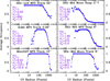 |
Fig. B.1 Examples of average occupancy versus (u, v) radius (filled circles) for different facilities, observing strategies and target beam FWHM. The fit to o(r) is overlaid as the solid line and parameter values are listed. |
Appendix C Other facilities
Here, we demonstrate the improvement in dirty PSF properties when using the AUW strategy for a variety of other upcoming and existing synthesis imaging arrays.
All Figures
|
Fig. 1 Comparison of restored image fidelity with standard UW, BRI, NA, and AUW for a noise-less (top-left), low-noise (top-right), nominal-noise (bottom-left), and high-noise (bottom-right) monochromatic 4-hour tracking observation with SKA-Low. The image fidelity has been averaged in logarithmically spaced annuli. |
| In the text | |
|
Fig. 2 Sky model used for image fidelity simulations. The full 6.4 × 6.4 degree field tapered with the primary beam model is shown on the left and the central portion on the right. The peak brightness is 1.5 Jy/Beam, the diffuse emission plateau has brightness of 0.2 mJy/Beam (about 25 K), and the faintest discrete sources are <1 µJy/Beam. |
| In the text | |
|
Fig. 3 Comparison of imaging performance with standard UW (dashed lines) and AUW (solid lines) for SKA-Mid. The monochromatic case is on the left and multi-frequency synthesis with 40% fractional bandwidth on the right. Bottom panels show the image RMS noise relative to NA weighting. The other panels show the RMS residual after a Gaussian fit to the PSF for a snap-shot (top) and full track (centre) observation. |
| In the text | |
|
Fig. B.1 Examples of average occupancy versus (u, v) radius (filled circles) for different facilities, observing strategies and target beam FWHM. The fit to o(r) is overlaid as the solid line and parameter values are listed. |
| In the text | |
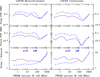 |
Fig. C.1 As in Figure 3 for the International LOFAR telescope. |
| In the text | |
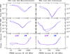 |
Fig. C.2 As in Figure 3 for SKA-Low. |
| In the text | |
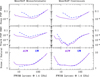 |
Fig. C.3 As in Figure 3 for MeerKAT. |
| In the text | |
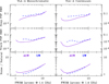 |
Fig. C.4 As in Figure 3 for the VLA A-configuration. |
| In the text | |
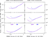 |
Fig. C.5 As in Figure 3 for ALMA (Cycle 10-8 configuration). |
| In the text | |
Current usage metrics show cumulative count of Article Views (full-text article views including HTML views, PDF and ePub downloads, according to the available data) and Abstracts Views on Vision4Press platform.
Data correspond to usage on the plateform after 2015. The current usage metrics is available 48-96 hours after online publication and is updated daily on week days.
Initial download of the metrics may take a while.