| Issue |
A&A
Volume 702, October 2025
|
|
|---|---|---|
| Article Number | A84 | |
| Number of page(s) | 17 | |
| Section | Planets, planetary systems, and small bodies | |
| DOI | https://doi.org/10.1051/0004-6361/202555184 | |
| Published online | 09 October 2025 | |
SOAPv4: A new step toward modeling stellar signatures in exoplanet research
1
Instituto de Astrofísica e Ciências do Espaço, Universidade do Porto, CAUP, Rua das Estrelas, 4150-762 Porto, Portugal
2
Département d’astronomie de l’Université de Genève, Chemin Pegasi 51, 1290 Versoix, Switzerland
3
Departamento de Física e Astronomia, Faculdade de Ciências, Universidade do Porto, Rua do Campo Alegre, 4169-007 Porto, Portugal
★ Corresponding author.
Received:
16
April
2025
Accepted:
13
July
2025
Abstract
Context. In the era of high-resolution spectroscopy, methods for characterizing exoplanets and their atmospheres are advancing rapidly. As these techniques are refined and allow for the detection of even the most minute signals from the planet, however, the role of the host star becomes increasingly significant. The characterization of planetary systems relies not only on methods targeting the planet itself, but also on a detailed understanding of the host star and its activity at the spectral level.
Aims. We present and describe a new version of the spot oscillation and planet code, SOAPv4. Our aim is to demonstrate its capabilities in modeling stellar activity in the context of RV measurements and its effects on transmission spectra. To do this, we employed solar observations alongside synthetic spectra and compared the resulting simulations.
Methods. We used SOAPv4 to simulate photospheric active regions and planetary transits for a Sun-like star hosting a hot Jupiter. By varying the input spectra, we investigated their impact on the resulting absorption spectra and compared the corresponding simulations. We then assessed how stellar activity deforms these absorption profiles. Finally, we explored the chromatic signatures of stellar activity across different wavelength ranges and discussed how such effects have been employed in the literature to confirm planet detections in radial-velocity measurements.
Results. We present the latest updates to SOAP, a tool developed to simulate active regions on the stellar disk while accounting for wavelength-dependent contrast. This functionality enables a detailed study of chromatic effects on radial-velocity measurements. In addition, SOAPv4 models planet-occulted line distortions and quantifies the influence of active regions on absorption spectra. Our simulations indicate that granulation can introduce line distortions that mimic planetary absorption features, potentially leading to misinterpretations of atmospheric dynamics. Furthermore, comparisons with ESPRESSO observations suggest that models incorporating non-local thermodynamic equilibrium effects provide an improved match to the absorption spectra of HD 20945 8 b, although they do not fully reproduce all observed distortions.
Key words: planets and satellites: atmospheres / stars: atmospheres / planetary systems
© The Authors 2025
 Open Access article, published by EDP Sciences, under the terms of the Creative Commons Attribution License (https://creativecommons.org/licenses/by/4.0), which permits unrestricted use, distribution, and reproduction in any medium, provided the original work is properly cited.
This article is published in open access under the Subscribe to Open model. This email address is being protected from spambots. You need JavaScript enabled to view it. to support open access publication.
1 Introduction
The connection between planets and their host stars is fundamental for characterizing planetary systems in detail. Stars are dynamic celestial bodies, and the signals we observe, both in terms of photometric and radial velocity (RV) studies, are equally complex. The main photospheric sources of these signals are stellar spots, faculae, and granulation for solar-like stars. Time series of active stars that are obtained with different techniques can be used to understand and infer several stellar properties, such as the velocity of the star (e.g., Nielsen et al. 2017; Santos et al. 2024) or its magnetic cycle (e.g., Lovis et al. 2011; Gomes da Silva et al. 2012; Suárez Mascareño et al. 2016). In planetary studies, it is a significant challenge to separate these signals. A key research focus therefore is understanding the effect of various stellar phenomena on the detection and characterization of exoplanets.
Stellar activity can either mimic or hinder signals of planetary origin in photometry and RV measurements for the characterization of the planet (e.g., Lagrange et al. 2010; Korhonen et al. 2015; Andersen & Korhonen 2015) or its atmospheric detection (e.g., Rackham et al. 2018; Cauley et al. 2018; Chakraborty et al. 2024). To remove signals of stellar activity such as spots and faculae, and in particular, their effect on the modulation of RVs and photometry, the community often relies on the use of mathematical methods, such as Gaussian processes. These methods have yielded remarkable results, including the detection of L 98-59 b, a rocky warm planet with half the mass of Venus (Demangeon et al. 2021), and Proxima d, an Earthmass planet orbiting the closest star to the Sun (Faria et al. 2022). Even though Gaussian processes are now a ubiquitous tool in such studies, their limited physical motivation and the wide range of possible kernel choices highlight the need for further investigation to quantify potential biases and the risk of spurious detections. An additional challenge lies in mitigating the effects of stellar granulation. In photometry, granulation has been recognized as a limiting factor in the detection of Earth-like planets that transit their host stars (e.g., Barros et al. 2020; Sulis et al. 2020). In RV measurements, the issue is equally critical. For a solar-Earth analog system, the granulation-induced RV signal is expected to reach approximately 80 cm s-1 (Meunier et al. 2015)1, whereas the planetary signal is anticipated to be only about 9 cm s-1.
The effect of stellar activity on the characterization of exoplanet atmospheres remains poorly explored. The majority of existing models is designed for low-resolution studies, in particular, spectrophotometric observations (e.g., MacDonald & Madhusudhan 2017; Rackham et al. 2018; Boldt et al. 2020; Mac-Donald 2023; Zhang et al. 2025). While these models provide valuable insights into stellar activity (e.g., Oshagh et al. 2013; McCullough et al. 2014; Petit dit de la Roche et al. 2024), their applicability to high-resolution studies remains limited. Furthermore, systematic studies of the impact of stellar activity on transmission spectra are lacking, and only a few works addressed specific aspects such as the effect of unocculted spots in low resolution by Rackham et al. (2018) and the influence on a limited set of high-resolution spectral lines by Cauley et al. (2018). A comprehensive systematic framework is needed to assess the full spectral impact of stellar activity.
Quiet stars also pose problems for planetary characterization and have to be accurately modeled, in particular, during transits. As a planet moves across the stellar disk, it occults stellar regions with varying local stellar spectra. These variations in the observed local spectra over the surface of a star are known as the center-to-limb variations (CLVs). The main sources of these changes include the projected stellar rotation2, the differing line profiles, and the flux variations (also known as limb-darkening). The latter two effects result from observations of stellar regions at different depths within the photosphere. It has been shown that CLVs are important to properly model the planet-occulted spectra during transits (Casasayas-Barris et al. 2020, 2021; Dethier & Bourrier 2023), with implications for the proper interpretation of planet transmission spectra.
Several studies have aimed to model these processes, and most adopted numerical approaches. Notable examples include previous SOAP versions (Boisse et al. 2012; Oshagh et al. 2013; Dumusque et al. 2014; Akinsanmi et al. 2018; Serrano et al. 2020; Cristo et al. 2024), which simulated the effects of stellar activity and planetary transits, the code called evaporating exoplanets (EVE) (e.g., Bourrier & Lecavelier des Etangs 2013; Dethier & Bourrier 2023), which is able to simulate the effect of atmospheric escape in exoplanets, and StarSim (Herrero et al. 2016; Rosich et al. 2020), which models stellar activity and its impact on observed spectra. Additionally, the code called numerical empirical Sun-as-a-star integrator (NESSI) (Pietrow & Pastor Yabar 2024) uses solar observations to compute solar-integrated spectra and study the impact of activity.
We present a new version of SOAP, hereafter SOAPv43. This code builds on previous versions by adding the possibility to add real spectra for each stellar region. This allows us to simulate the spectroscopic and photometric time series of a planet that transits its host star and the signature of stellar activity.
This paper is structured as follows. Sect. 2 discusses the previous evolution of SOAP and details the new features that were introduced over time and in this version in more detail. In Sect. 3 we present applications of SOAPv4 that show its potential for planetary transit modeling, including comparisons of absorption profiles with solar observations, analyses of the transit spectroscopy dataset of HD 209458 b, and its capability to model active regions at the spectral level. Finally, Sect. 4 summarizes the key aspects of this new version, highlights its limitations, and outlines prospects for future development.
2 SOAPv4
2.1 SOAP development through time
The code SOAP (Boisse et al. 2012) was initially developed to simulate the impact of stellar activity (e.g., starspots) on RV time series. The code simulates this by approximating the local stellar disk spectrum using a cross-correlation function4 (CCF), modeled as a Gaussian profile with user-defined parameters. The CCFs at different locations on the stellar surface are Doppler-shifted according to local velocities, assuming solidbody rotation, and flux-weighted following a limb-darkening law. Active regions are simulated by initially placing a circular region, defined in terms of the stellar radius, at the disk center. This region is then mapped to the specified latitude and longitude using spherical symmetry. The same Gaussian profile is applied to the CCFs of active regions. In terms of the flux contribution, the CCFs of active regions are weighted by their contrast: Values between 0 and 1 for dark spots, and values greater than 1 for bright faculae5.
Each successive version of SOAP was then built upon the previous framework. SOAP-T (Oshagh et al. 2013) incorporated the effect of planet orbiting the star. In particular, the simulation accounts for the planet-occulted stellar regions during transits by subtracting the quiet-star (QS) pixels behind the planet at each position in the time series. This enhancement allows the code to simultaneously model the photometric light curve and the Rossiter-McLaughlin effect (Holt 1893; Rossiter 1924; McLaughlin 1924) in addition to the Keplerian motion. This expands its applications to understand the architecture of planetary systems better.
SOAP2.0 (Dumusque et al. 2014) was built upon the first version of the code (without planetary transits) to refine the physics of active regions. This version enables the use of solar observations to simulate stellar activity, specifically, by incorporating data from the Fourier Transform Spectrograph (FTS) at the Kitt Peak Observatory. It includes observations of the QS at the disk center (Wallace et al. 1998) and an umbral region of a sunspot (Wallace et al. 2005), which allows a more realistic modeling of the stellar activity, at least in the solar case. These observations account for line-profile deformations induced by stellar activity, including the effects of convective blueshift6 and its inhibition in active regions. Additionally, this version incorporates facu-lar limb brightening and a realistic contrast ratio for spots and faculae by computing the flux contrast based on the Planck distribution at different temperatures between active regions and the quiet photosphere. SOAP2.0 remains limited to using CCFs as in previous versions, however, and it is unable to generate realistic spectra.
The subsequent versions of the code were not publicly released, but played a crucial role in the development of SOAPv4. The advancements from SOAP-T and S0AP2.0 were integrated by Oshagh et al. (2016) to study the impact of stellar activity on the measured misalignment of exoplanets. Later, Akinsanmi et al. (2018) enhanced the code to simulate the effects of a ringed planet and rotational deformation on the photometric transit light curve and the RV signal in the Rossiter-McLaughlin effect. More recently, Serrano et al. (2020); Cristo et al. (2024) incorporated the effects of differential rotation (e.g., Balona & Abedigamba 2016), while Cristo et al. (2024) added the convective blueshift signal that can be observed during planetary transits (Shporer & Brown 2011).
In addition to the main development line of the code, a fork of S0AP2.0, SOAP-GPU (Zhao & Dumusque 2023), was created to simulate spectra. This version focuses on refining the stellar activity modeling by incorporating improvements such as direct mapping of active regions to account for complex shapes and a more advanced treatment of variations in the convective blueshift profile across the stellar disk, based on the measurements of Löhner-Böttcher et al. (2019). Furthermore, the code has been optimized for GPU execution, which significantly improved the computational efficiency compared to the original version. The requirement of a GPU architecture poses a usability challenge for most users, however. Furthermore, SOAP-GPU does not include the possibility of modeling a transiting planet.
2.2 The fundamental structure
The SOAP code uses a numerical approach to simulate various aspects of stellar activity and planetary signals in astronomical measurements. In this new version, we have followed the main development trajectory by integrating all previous upgrades and extending its capabilities beyond photometry and CCFs to also model the time series of spectra. The first step of the algorithm involves constructing the QS. This process involves projecting the stellar disk onto a square grid with side length n, resulting in a total of N (n × n) grid points (see Fig. 1). The next step selects the points within the stellar disk based on their position inside a unit disk, which is determined by calculating the distance between the centroid of each grid point and the center of the stellar disk. The position associated with each point is then used to compute the relevant physical quantities described below.
For each pixel in the grid, the flux contribution is determined by a limb-darkening law, and the corresponding coefficients are provided as inputs to the code. The total integrated flux at each time step is calculated by summing all grid pixels.
The signal of a transiting planet, after its relative position to the grid is computed, is obtained by recomputing the QS signal of the cells behind the planet and subtracting from the QS integrated signal. For an active star, the flux contribution from active regions (ARs) is determined based on their position within the grid and its contrast relative to the QS. In the code, an AR is characterized by four parameters: latitude, longitude, radius ratio relative to the star, and temperature contrast.
Initially, an AR is placed at the center of the stellar disk, and its boundaries are defined by its radius. Subsequently, the ARs are translated into spherical coordinates according to the initial input parameters. In a time-series simulation, their coordinates are dynamically updated based on the observational phase, which is coupled to the stellar rotation.
At each time step, the code uses a precomputed bounding box around the AR position (illustrated in Fig. 2). To determine the effect of the AR on the total integrated stellar signal, the code iterates over all grid points within the precomputed bounding box. Because the AR shape becomes distorted after projection onto the observed stellar disk, however, its precise geometry in the final coordinate system is unknown. To address this, the code applies an inverse rotation, for which it effectively shifts the AR back to the disk center, where its shape is well defined. This approach ensures that the QS signal can be accurately computed and subtracted from the original integrated stellar signal and that the specific contribution of the AR is isolated. Finally, the signal at the AR position is recalculated by multiplying the contrast between the star and the AR (calculated using Planck’s law) with the limb-darkening effect (Boisse et al. 2012; Dumusque et al. 2014). For a transiting exoplanet, the code includes a condition to exclude the contribution of any AR located behind the planet. This optimization improves computational efficiency because the signal from these ARs would ultimately be removed.
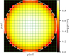 |
Fig. 1 Depiction of the SOAP projection of a stellar disk onto a grid of 20 × 20 pixels for illustration purposes. The color map represents the local normalized flux in each position, which is determined by the limb-darkening. The white circumference outlines the original disk for reference. |
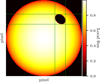 |
Fig. 2 Position of a spot with a radius of 15% of the stellar radius at a latitude and longitude of 45° and projected onto a 300 × 300 pixel grid. The vertical and horizontal green lines indicate the precomputed bounding box that marks the minimum and maximum Cartesian coordinates within the grid. The brown points represent the calculated positions that define the spot boundary in its final projected location. |
2.3 What is new in SOAPv4
With SOAPv4, time-series simulations of CCFs and spectra are inherently linked. Since a CCF is derived as a weighted average of spectral lines based on a reference mask (e.g., Baranne et al. 1996; Pepe et al. 2002), its computation is directly tied to the underlying spectra. Given this relation, we primarily focus on describing how the code simulates spectra, while details of CCF calculations can be found in Boisse et al. (2012) and Dumusque et al. (2014).
A summary with the key differences between the versions is provided in Table A.1.
2.3.1 The quiet-star spectrum
The QS spectrum of a simulated star can be computed by integrating the local spectra of the star in different disk positions. These in turn depend on three key inputs: the local spectra, the local velocities, and the flux distribution across the stellar disk. The local spectrum is mainly determined by stellar properties such as effective temperature, metallicity, surface gravity, and other atmospheric parameters.
From a modeling perspective, each pixel in the grid must be assigned a spectrum that accurately reflects the local conditions of the star. To provide flexibility, the code allows users to specify this spectral information in various ways (Table B.1 summarizes some of the options employed below). Users can input synthetic stellar spectra, such as those from the PHOENIX library (PHNX; Husser et al. 2013), or spatially resolved spectra across the stellar disk (e.g., generated with Turbospectrum; Plez 2012), computed under either local thermodynamic equilibrium (LTE; model TS-LTE) or nonlocal thermodynamic equilibrium (NLTE; model TS-NLTE) conditions. Alternatively, observed spectra may be used, including solar spectra employed in the SOAP2.0 CCF calculations for the quiet-Sun disk center (FTS-QS) or high-resolution spectra from the IAG atlas of the spatially resolved quiet Sun (IAG; Ellwarth et al. 2023)7. Both the IAG and TS provide spectra as a function of disk position, capturing variations in the line profiles across the stellar surface. For the purposes of describing the code, we assumed that a single spectrum is applied to each grid element. This method can readily be extended to account for μ-dependent spectra (where μ corresponds to the limb angle), however.
The input spectrum, which can optionally be normalized, is then convolved with the instrumental profile at a resolution specified by the user.
Each spectrum in the grid is Doppler shifted according to the local velocity of the star, incorporating effects such as differential rotation and convective blueshift, as described by Serrano et al. (2020) and Cristo et al. (2024). Finally, the spectrum is interpolated back to the original wavelength grid, and its flux is rescaled according to the disk position using a wavelength-dependent limb-darkening prescription. This step is optional in series of μ-dependent spectra where the intensities are known. A specific example of how local spectra can vary as a function of limb angle is shown in Fig. 3. The integrated quiet-star spectrum is then obtained by summing the contributions from all grid elements corresponding to the visible stellar disk.
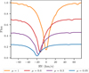 |
Fig. 3 Local line profiles centered on the sodium D2 line at different limb angles for a solar-like star that rotates as a solid body at 20 km s-1. The representation illustrates velocity variations from the disk center to the eastern limb for a star rotating from west to east. As the pixels approach the limb, the flux decreases due to limb darkening, while the projected velocity component increases. |
2.3.2 Including active regions
For an active star, as described in Section 2.2, the code identifies the region of the grid occupied by the active region (AR) or ARs at each time step and for each set of location angles. The activity component can consist of a single AR or a list of ARs, each with its own set of properties that evolve over time according to the stellar rotation.
The spectral contribution of the active region at each pixel is computed using a potentially different input spectrum (the choice is given to the user). One example is a synthetic spectrum, such as PHNX, which matches the temperature of the AR to capture spectral variations induced by temperature changes. In Fig. 4, we present the effect of temperature variations on the line profiles in the Na I doublet region, adopting solar properties as the reference baseline (see Table C.1). The lower temperature of star spots leads to broader spectral lines than in the surrounding photosphere, whereas the higher temperature of faculae produces narrower lines. Consequently, cooler active regions predominantly affect the wings of the integrated spectral lines, while hotter regions exert a more significant influence on the line core.
When the spectral intensities are unknown, the flux contrast between the QS and the AR cannot be directly determined. In these cases, the code estimates the flux ratio by computing the ratio of the Planck distribution at a reference wavelength for the effective stellar temperature and that of the AR temperature, following a similar approach to that used at the CCF level.
For input spectra where intensities are known, SOAP operates with normalized fluxes. This is accomplished by normalizing the spectra to the maximum stellar flux within a specified wavelength interval8, and scaling the AR spectrum to the same reference level at the corresponding wavelength. This wavelength is provided as an input parameter to the code to ensure that contrast is correctly maintained and that chromatic contrast is preserved in the simulations.
When a planetary transit is simulated, we follow the method described by Oshagh et al. (2016), wherein the local signal of the QS behind the planet is computed and subsequently subtracted from the integrated QS signal. During the planetary transit, the AR signal is not calculated at the occulted positions to avoid unnecessary computational overhead.
Additionally, the RV signal, along with spectral indicators such as the full width at half maximum (FWHM) and bisector inverse slope (BIS), can be directly computed from the spectra using the CCF method. At the simulation level, the code allows users to input a cross-correlation template that specifies the wavelengths and weights, which can be a simulated spectrum, weighting function, or binary mask. The code then cross-correlates this template with the time series of the integrated spectra and produces a series of CCFs. The RVs are determined by fitting a Gaussian function to each CCF, while the FWHM and BIS indicators are computed directly from the CCFs.
To assess the performance of the code in simulating active regions, we compare the CCF results of S0APv4 with those of S0AP2.0 in Appendix E. In these simulations, we computed the variations in RV, BIS, and FWHM induced by two active regions with a 1% filling factor for a solar analog: a cool spot with a temperature 663 K below the photospheric value, and a facula whose temperature contrast follows the empirical law of Meunier et al. (2010), which is 34.1 K hotter than the photosphere at the disk center and increases to 209.5 K near the limb. The results are generally consistent, but a discrepancy is observed at the centimeter per second level. This difference has been verified to stem from modifications in the interpolation method and the selection of grid points. These adjustments are anticipated to yield more accurate results because they more effectively approximate the derivative of the line at the first point and, in the second instance, reduce the grid error to half a pixel.
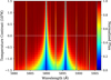 |
Fig. 4 Variation in the sodium doublet line properties as a function of temperature contrast in regard to the solar case. Positive contrasts correspond to spectra of faculae, and negative contrasts represent spectra of spots. The quiet-star spectrum is indicated by the dashed white line at the zero level. All spectra used to construct the figure were taken from the PHOENIX library. |
3 Applications
This section demonstrates the versatility and capabilities of the S0APv4 model through several key applications. We explore how this tool can be used to interpret transmission spectra, model stellar activity, and distinguish between stellar activity signals and other spectral features. First, we examine the model performance in simulating the HD 209458 system, with particular focus on the sodium (Na) doublet region where atmospheric detection has been debated in the literature (to be discussed in Section 3.2). We then use spatially resolved IAG spectra to validate the model against solar benchmark data and assess the effect of different model parameters on the simulated signals. The section also investigates the critical impact of stellar activity on transmission spectra by simulating spot-crossing events and analyzing their spectral signatures. We demonstrate that spots can create distortions in absorption profiles that might be misinterpreted as planetary atmospheric features. Finally, we show that S0APv4 can model chromatic RV variations caused by stellar activity. This makes it a valuable tool for distinguishing between stellar activity and genuine planetary signals. Through these applications, we illustrate that SOAPv4 serves as a comprehensive framework for investigating the complex interplay between stellar features and planetary signals in exoplanet characterization studies.
For the simulations presented in the following subsections, we adopted a grid size of 800, which is generally sufficient to accurately model transits of hot-Jupiter-sized planets and active regions with sizes of about 1%. Table B.1 summarizes the key properties of the input spectra we used in these simulations.
3.1 Solar simulations
Due to its proximity with Earth, the Sun provides a unique opportunity to gain detailed insights into its dynamics and to use it as a testbed for various models and extraction techniques. Furthermore, its observations can serve as a benchmark for the model validation because high-resolution observations of different regions of the solar disk allow direct comparisons. As new models emerge in the literature that depend on local phenomena in the stellar disks, it is crucial to first evaluate their performance against the solar case.
In this subsection, we employ spatially resolved solar observations from IAG, along with PHNX and μ-dependent TS-LTE and TS-NLTE, to simulate the expected absorption signal caused by planet-occulted line distortions (POLDs) using SOAPv4. A similar study was reported by Reiners et al. (2023) for the HD 189733 system. These results, however, only offer an order of magnitude for this specific case, however, because the star is considerably cooler than the Sun (4969 ± 48 K; Sousa et al. 2021). We chose to model a scenario of a typical hot Jupiter orbiting a solar analog.
The IAG spectra result from observations using the Fourier Transform Spectrograph (FTS) at the Institut für Astrophysik und Geophysik (IAG) in Göttingen. The observation were conducted with a 32.5" fiber size, observing 14 μ positions that ranged from disk center to very close to the stellar limb. It is important to note, however, that because the physical size of the fiber used in observations is finite, each recorded profile is not strictly spatially localized. This effect becomes more pronounced toward the stellar limb, where the increased overlap between different μ-angles results in greater deviations.
3.1.1 Inactive solar analog
We investigated the POLDs associated with the Na I D lines because they are among the most extensively studied alkali metal features in the optical regime (e.g., Charbonneau et al. 2002; Sing et al. 2008; Langeveld et al. 2022; Seidel et al. 2023). Their typically deep and broad profiles make them favorable for detection, and they have therefore been a prominent target in the literature.
We defined the physical parameters for a Jupiter-like planet orbiting at 9 R⊙, corresponding to an orbital period of approximately 3.13 days. The remaining stellar parameters were assumed to be solar and are listed alongside the planetary parameters in Table C.1. We modeled the star assuming rigidbody rotation throughout the simulations. For the solar spectra, we employed four distinct sources: PHNX, IAG, TS-LTE, and TS-NLTE.
For the simulation using IAG data (and, by extension, for those employing the other input spectra used for comparison), we focused on the Na I D1 line. The Na I D2 line is heavily contaminated by neighboring lines, which are masked in the atlas. Consequently, the line profiles are affected by this and possible leftover spurious signals, which may introduce bias in the conclusions that are drawn. For the D1 line, however, most of the line structure is preserved (see Fig. 5).
For the simulations, we used normalized spectra or prenormalized all input spectra. It is common practice to normalize spectra by the continuum to compute transmission spectra, in particular, because modern high-resolution spectrographs typically lack flux calibration. Caution is warranted, however, because the choice of local normalization method can significantly influence the resulting transmission spectrum9. For consistency, we selected the same wavelength intervals around the sodium lines for normalization in this study.
For PHNX spectra, the normalization was performed automatically by SOAPv4. The code selected flux points that corresponded to the outermost 10% of the chosen intervals and rejected any spectral lines within this subinterval. IAG, TS-LTE, and TS-NLTE provided prenormalized outputs.
In Fig. 6 we show the resulting planetary absorption spectra10 obtained from SOAPv4 simulations using the different stellar spectra sources. The absorption simulation from IAG spectra exhibits the highest absorption at the wings. At the core, however, the emission is weaker than in the TS-LTE and TS-NLTE stellar atmosphere models. Neither the TS nor the PHNX simulations are able to reproduce the asymmetry that is observed with the IAG absorption spectrum. This suggests that the asymmetry is not driven by CLVs caused by the differences in line shape by varying atmospheric depths that are observed at different μ-angles, nor is it caused by NLTE effects.
A key effect that is currently missing in SOAPv4 and most models available in the literature, but s present in the IAG spectra due to their observational nature, is granulation11. Granulation distorts the stellar spectra locally due to the three-dimensional effect of observing granules from different perspectives, and it captures various components of the convective flows within the granular structure. This phenomenon has also been noted by Reiners et al. (2023).
Although CLVs do not explain the observed asymmetry, they remain an important factor in modulating the absorption signal. The constant PHNX model exhibits the largest deviation from IAG in terms of signal amplitude of the simulated profiles. The TS models provide a better approximation, but the LTE version retains residual absorption in the wings, whereas the NLTE version matches the IAG better. This indicates that NLTE effects cannot be neglected.
When we consider the IAG-simulated absorption profile as the reference model spectrum, it becomes evident that current modeling techniques face significant challenges. In particular, the TS LTE and NLTE models both overestimate the emission signal at the core. Because the absorption spectra are presented in the planetary rest frame, we might be inclined to attribute the observed signal to absorption originating from the exoplanet atmosphere. Furthermore, the asymmetry of the profile might be misinterpreted as evidence of atmospheric winds.
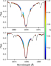 |
Fig. 5 IAG Na I D2 (top) and Na I D1 (bottom) Na I lines as a function of limb position. The wavelength interval was selected to represent a 3 Å region surrounding each line. Contaminated regions that are affected by neighboring lines were excluded, as demonstrated by the comparison with the integrated star spectrum shown in black. |
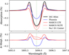 |
Fig. 6 Comparison of the absorption spectra generated using SOAPv4 for a solar analog hosting a hot Jupiter. The top panel presents a comparison of the absorption profiles obtained using input spectra from IAG, TS, and PHNX spectra that matched the stellar properties. The bottom panel illustrates the differences between the absorption spectrum produced with IAG and the spectra derived from the other models. These simulations represent the POLDs centered on the Na I D1 line and span a wavelength range of 1 Å on either side. |
3.1.2 Stellar activity
Stellar activity has recently become a key focus in the context of atmospheric characterization. As discussed in the introduction, most studies primarily investigated the impact of stellar activity on broadband transmission spectra or were limited in the number of features that were analyzed at higher resolution. SOAPv4 serves as a valuable tool for exploring the effects of stellar activity on high-resolution transmission spectra by assessing how different active regions influence the extracted signals and determining how the resulting biases can be mitigated or accounted.
For these simulations, we considered a system as described in the previous section and set a spot-crossing event scenario. The simulations were based on PHNXspectra, where the properties of the QS spectrum are identical to those of the Sun, while the spot was modeled as being 663 K cooler than the stellar surface (Lagrange et al. 2011). Additionally, we tested simulating the absorption spectra with observed spectra from the FTS at the Kitt Peak Observatory, including spectra from the quiet Sun at disk center (Wallace et al. 1998) and an umbral sunspot region (Wallace et al. 2005) for comparison.
We simulated a starspot with a filling factor of 0.5% at a latitude of -30° and a longitude of -35°, and we ensured that it was occulted during the transit. Furthermore, we introduced an impact parameter (b) of -0.6 to approximate the orbital inclinations of systems such as HD 189733 or HD 209458 (see the system architecture in Appendix C, Fig. C.1).
By default, SOAPv4 computes and provides the transmission spectrum time series in the stellar rest frame by dividing the in-transit spectra by an out-of-transit spectrum. To shift it into the planetary rest frame, we first computed the planet velocities at the simulation phases and then applied a Doppler shift to remove these velocities, followed by an interpolation onto the original wavelength grid.
In Fig. 7 we present a comparison between simulations with and without the spot contribution, using two input spectra: PHNX and FTS. Additionally, Fig. C.2 illustrates the time series of absorption spectra in the stellar rest frame for the PHNX spectrum simulation. Although the PHNX and FTS spectra are at the same temperature, the difference in amplitude between the simulations of the two models is significant. This is already visible at the input level of the spectra. The observed spectra have broader and deeper lines on average than the observations (Fig. C.3)12.
Regardless of the model, the subtraction of the scenario without a spot from the scenario with a spot reveals a distortion in the absorption spectrum that amounts to a significant percentage of the original absorption profile (see the lower panel of Fig. 7). Locally, the continuum level of the spectral line appears to change and gradually approaches zero. This effect directly reflects the spectral profile of the star spot, which is broader than that of the quiet stellar surface. Over a broader wavelength range, however, broader than the width of the spectral spot lines, this apparent change in the continuum vanishes.
To the left of the line center, a redshifted feature appears in the difference between the model spectra. For the PHNX spectra, the quiet-star scenario exhibits a stronger absorption feature than the spot-crossing event. This outcome is expected to some extent because the local flux contrast distorts the line profile on the blueshifted side of the star.
In contrast, however, a similar structure appears in emission at approximately the same wavelengths in the FTS spectra. This discrepancy may arise from the relative behavior of the spectral lines: while the QS spectrum in PHNX is shallower than that of the spot, the opposite is observed in the FTS spectra.
This feature is well constrained within the absorption spectrum, and this may pose challenges for interpreting planetary atmospheric signatures in active stars. Its core is shifted from the expected velocity by less than 10 km s-1, which is comparable to typical atmospheric dynamics. Repeated transit observations might help us to distinguish the origin of these deviations, however, provided that active regions evolve significantly between observations.
It is crucial to emphasize that we simulated a highly specific scenario. Variations in the location of active regions and differences in the orbital architecture of exoplanetary systems are expected to affect the resulting absorption profiles significantly. This underscores the importance of developing computational tools capable of assessing the contamination of planetary signals by stellar activity. In particular, the objective of the code SOAPv4 is to provide a robust and flexible framework for a comprehensive analysis of this issue.
A single transit observation may still allow us to identify a spot-crossing event at the level of the absorption spectrum. Photometric and spectroscopic transit observations are often combined to enhance the detection capabilities. These complementary data are not always available, however, and it can be challenging to identify spot crossings based on RV measurements alone. Nevertheless, the residual asymmetry in Fig. 7 correlates with the spot position on the stellar disk.
Typically, constructing the absorption spectrum involves averaging the local absorption profiles along the transit chord, possibly excluding the ingress and egress regions, as discussed above. Under certain conditions, however, it may be feasible to separately average the profiles from T2-Tcenter and from Tcenter-T3. In a scenario that is perfectly parallel to the stellar equator, such as the we presented here, the resulting absorption spectra should be fully antisymmetric because the planet covers regions with the opposite velocities and spectral profiles. To test this, we divided the absorption profiles in these intervals and compared them with the QS scenario (Fig. 8).
The simulated spot was located on the leading stellar hemisphere, corresponding to the regions probed by the planet at T2-Tcenter (blue lines in the figure). The effect of the spot crossing is clearly stronger than in Fig. 7, primarily because of two factors. First, the averaging was performed exclusively in the blueshifted region of the star, which resulted in spectral lines with more similar positions. Second, the fraction of the spot signal relative to the overall absorption signal is larger. Compared to the QS scenario, a blueshifted signature is again observed in the difference between the two profiles. Furthermore, the local continuum exhibits additional absorption, which arises from the broader profile of the spectral lines of the spot. No significant features are observed in the trailing hemisphere. The local continuum does not reach the zero level because contamination from the spot remains present in the background from the construction of the master-out spectrum.
In the presence of stellar activity, the choice of the reference spectrum for comparison becomes particularly important. If the ratio of the transit duration and the stellar rotation speed is low (typically the case for slow rotators), there change in the velocity during observations is minimal to displace the spectrum of the active region. As a result, the contamination from active regions remains quasi-static and is effectively averaged out (but not removed, as we have shown) over the quiet star. When this ratio is sufficiently high, however dynamical effects may become apparent and superimpose themselves on the POLDs. They might even manifest themselves in out-of-transit observations.
This effect can be exacerbated by the method that is currently used to construct transmission spectra. Typically, out-of-transit integrated stellar spectra are aligned and corrected for systematic velocity trends by applying RV corrections that are derived from a fit to the observed velocities. Active regions not only induce genuine Doppler shifts, however, but also introduce distortions in the spectral lines. These distortions can be misinterpreted as velocity shifts, in particular, when methods such as the crosscorrelation function (CCF) are used, and this might lead to a misalignment of the master-out spectrum. This misalignment can introduce spurious effects in the in-transit comparison and might distort the inferred transmission spectrum.
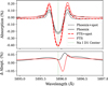 |
Fig. 7 Top panel: full absorption profiles for the PHNX (blue) and FTS (red) input spectra without active regions (solid lines), together with the corresponding profiles with a stellar spot (dashed lines). Bottom panel: differential signals obtained by subtracting the quiet-star profiles from the spot-crossing profiles. The color-coding matches the input spectra. The wavelength interval is the same as in Fig. 6. |
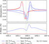 |
Fig. 8 Comparison of partial mean absorption spectra for QS and spotcrossing events. In the top panel, the profiles for the two scenarios are presented. The leading hemisphere profiles (blueshifted) are represented in blue and the trailing hemisphere profiles (redshifted) are shown in red. The bottom panel shows the difference between the partial profiles for the quiet-star and spot-crossing events. The same wavelength interval as in Fig. 6 is used. |
3.2 Transmission spectrum of HD 209458
HD 209458 A is a bright solar-type star with a visual magnitude of 7.63 (Høg et al. 2000) and is classified as spectral type F9V (Gray et al. 2001). It hosts the exoplanet HD 209458 b, whose size is similar to that of Jupiter, but has only two-thirds of its mass. The favorable planet-to-star radius ratio, along with the extended nature of its atmosphere, makes HD 209458 b one of the most important targets for atmospheric characterization studies.
This planet was originally proposed to host the first detected atmosphere, inferred from an excess absorption in the sodium doublet region reported by Charbonneau et al. (2002). Since then, the authenticity of this detection has been a subject of ongoing debate. In low-resolution studies, Sing et al. (2008); Snellen et al. (2008); Santos et al. (2020) confirmed this detection, whereas Casasayas-Barris et al. (2020, 2021) showed no evidence of an atmospheric signature in high-resolution observations. More recently, Carteret et al. (2024) showed based on simulations that the absorption feature that was observed in low-resolution by Charbonneau et al. (2002) could not be explained by the effect of stellar rotation on the transmission spectrum. A plausible resolution to the paradox is that sodium absorption in the atmosphere of HD 209458 bmainly arises from the pressure-broadened wings of the Na I D doublet, which formed in deeper, high-pressure layers. These broad wings can span several nanometers and appear as shallow but wide features in low-resolution spectra, which makes them detectable over large bandpasses. In contrast, high-resolution spectra isolate the narrow-line cores, where absorption may be weak or absent because the Na abundance at high altitudes is low or because it is obscured by clouds or hazes, resulting in little to no signal at these wavelengths. In ground-based high-resolution observations, this absorption thus disappears as a result of the continuum normalization on the data.
We used SOAPv4 to simulate the sodium absorption feature that is expected from the deformation of the stellar lines by the planet during the transit. An accurate modeling of the stellar surface behind the planet is essential because the range of planetary velocities that are projected along the line of sight during the transit causes any potential atmospheric absorption signal to fall within the velocity range of the POLDs. Because the host star is in the hotter range of solar-type stars, it has been shown (Casasayas-Barris et al. 2021; Dethier & Bourrier 2023) that the the POLDs in high-resolution absorption spectra can only be accurately reproduced when NLTE effects in the spectral lines synthesis are accounted for. Therefore, we used synthetic spectra generated under NLTE conditions for the simulations to investigate the effect on the transmission spectrum.
To derive the transmission spectra from our simulations, we adopted the parameters listed in Table 1. One of the key parameters that significantly affects the amplitude of the POLDs is the stellar rotation speed, veq sin i (Dethier & Bourrier 2023). This parameter can be determined through various techniques, including stellar line broadening (e.g., Gray 2005), the analysis of stellar variability in photometric observations (e.g., Reinhold et al. 2013; McQuillan et al. 2014; Santos et al. 2024), and the Rossiter-McLaughlin effect (e.g., Hirano et al. 2011; Brown et al. 2017).
Additionally, the rotation of the stellar surface can be inferred by analyzing the missing spectral information of a star during a planetary transit (Brown et al. 2017). This technique has become increasingly common and is now frequently employed alongside transmission spectroscopy to refine the stellar parameters, such as the stellar rotation speed or differential rotation (e.g., Hoeijmakers et al. 2020; Casasayas-Barris et al. 2021; Steiner et al. 2023). One of the key advantages of SOAPv4 is its ability to self-consistently model the Doppler-shadow signal (e.g., Cegla et al. 2016; Dravins et al. 2017, 2018), which enables us to recover the transmission spectrum based on this information.
For this analysis, and to take into account the change in line shape as a function of the limb angle, we used Turbospectrum to produce synthetic spectra for a specific array of μ angles to be provided to the code. As parameters, we used the stellar physical properties in Table 1. Similarly to Casasayas-Barris et al. (2021), we tested models with both LTE and NLTE approximations, using a solar Na Iabundance, A*(NaI). Two main values are used in literature: 6.33 ± 0.03 (Grevesse & Sauval 1998) and 6.17 ± 0.04 (Grevesse et al. 2007). In Fig. D.1 we show the map of the local spectra in a wavelength interval between 5882 and 5902 Å, which encloses the Na I D1 and D2 lines.
We note that during transit, the profiles behind the planet change significantly due to CLVs. In the literature and for an observational analysis, however, it is common to average the transmission spectrum over the entire transit (T1-T4) or restrict it to the fully in-transit phases (T2-T3) to increase the signal-tonoise ratio. A restriction of the phase range to T2-T3 ensures that the planet remains entirely within the stellar disk, which avoids positions in which the μ angles are very close to the stellar limb. This is often challenging to model. In our simulation, we fixed the profiles to μ = 0.2 when the angle fell below this threshold.
In Fig. 9 we show the absorption spectrum as derived from ESPRESSO observations by Casasayas-Barris et al. (2021) for the sodium D1 and D2 lines, compared with the models obtained using SOAPv4. The models generated with NLTE spectra agree better with the absorption profile, in particular, to explain the shape of the wings and the amplitude of the feature.
For the absorption feature associated with the D2 line, the model reproduces the left wing more accurately than the right wing, where an apparent excess absorption is observed relative to the model. A similar trend is seen for the D1 feature, with a pronounced excess absorption in the left wing that the models fail to capture. Additionally, near the line cores, an absorption feature extending over approximately 0.1 Å is observed in both the D1 and D2 lines. A possible explanation for this excess absorption close to the absorption core was given by Dethier & Bourrier (2023), who modeled the effect of a planetary atmosphere containing Na I in its composition, which explained the additional absorption that is seen. In addition, the authors were able to explain the asymmetry that is observed by modeling an atmosphere with a thermosphere with a night-to-day side wind of around 3 km s-1.
For this showcase scenario, the model computed with SOAPv4 agrees well with the models used by Casasayas-Barris et al. (2020, 2021); Dethier & Bourrier (2023) and can explain the observations to a similar level of accuracy.
HD 209458. Stellar and planetary properties.
3.3 Application to RVs
Modeling stellar activity is crucial for planet detection and characterization through the RV method (Rauer et al. 2024) because it can obscure the signals of low-mass planets. Previous versions of SOAP addressed this by simulating the CCF at the pixel level, where the contrast between the quiet star and active regions was determined using a reference wavelength at which the Planck distribution ratio of the stellar and AR temperatures was computed. Although the same approach can be applied to small segments of spectra, it is generally more practical to compute the CCF over the full bandpass of an instrument.
In SOAPv4, it is now possible to simulate large portions of the spectrum while maintaining the contrast ratio of the star and ARs. This is achieved by normalizing the spectra to the maximum stellar flux and using the corresponding wavelength to scale the AR spectrum to the same reference value. The code then internally recalculates the appropriate flux level when it determines the local AR contribution and takes the temperature into account.
To illustrate the variation in the spot RV amplitude with wavelength, we simulated a time series of integrated spectra for a solar-type star as it would be observed with ESPRESSO. We considered a spot at the disk center with a 1 % filling factor and an effective temperature 663 K below the photosphere. In this case, we applied an average limb-darkening law derived using LDtK (Parviainen & Aigrain 2015) with the spectral library of Husser et al. (2013), integrated over the ESPRESSO bandpass, which spans 3800 and 7880 Å.
In Fig. 10 we present the RV time series obtained by crosscorrelating the solar PHNX model with several chromatic spectral bins of the active integrated star. These bins were constructed by dividing the initial interval into 70 intervals, each containing an equal number of points (with the exception of the last bin). A clear trend in amplitude is evident, with higher RV amplitudes observed at shorter wavelengths in the visible spectrum, and progressively lower amplitudes for longer wavelengths.
This trend in amplitude is known, and it is mainly a consequence of the energy distribution contrast between two sources at different temperature (e.g., Huélamo et al. 2008; Reiners et al. 2010). It was used as a tool to distinguish stellar activity from true planetary signals (e.g., Huélamo et al. 2008; Suárez Mascareño et al. 2020; Faria et al. 2022).
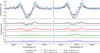 |
Fig. 9 Absorption profiles of the Na I D lines in HD 20945 8 compared against the observed absorption profile derived from ESPRESSO data, as presented in Casasayas-Barris et al. (2021). In the top row, the absorption points are shown in black, and their respective uncertainties are represented by a confidence interval (CI in the plot) band at the 1σ level. The absorption features computed using SOAPv4 are overplotted. They were based on input MARCS models with two Na I abundances (solar-like) reported in the literature. The subsequent rows display the residuals between the models and observations. The colors of the data points and CI bands correspond to the respective model color. |
 |
Fig. 10 RV curves computed using SOAPv4 for an equatorial spot with a 1% filling factor, which is 663 K cooler than the photosphere. The color bar represents the average wavelength of the spectral bins, from which the radial velocities were derived using the CCF technique with the QS solar PHNX model. |
4 Discussion and prospects
We have presented the most recent updates to the code SOAP and its applications at the spectral level. The current version, SOAPv4, is capable of simulating the effects of ARs at any position on the stellar disk, assuming a circular shape for the ARs when they are at the disk center. Additionally, SOAPv4 preserves the wavelength-dependent contrast, that is, the energy distribution difference between the star and the AR. This feature allows us to evaluate chromatic effects on RVs.
With respect to planetary transits, SOAPv4 proved to be a valuable tool for modeling the POLDs under a variety of input spectra, whether synthetic or observed, and for assessing the impact of active regions on absorption spectra. As an illustrative example, we showed that for a solar-analog star hosting a representative hot Jupiter, absorption spectra modeled with solar observations cannot be fully reproduced by synthetic spectra that share the properties of the Sun. We suggest that the asymmetry that is observed may in part be due to the granulation effect on the solar surface that distorts the spectral lines locally. Moreover, the distortion observed in the comparison may mimic an asymmetric planetary absorption feature. These distortions might not only lead to false detections, but might also generate spurious signatures of atmospheric dynamics. We note, however, that the difference between these simulations of absorption spectra is a function of the system properties, and the amplitude and distortion of the signal are expected to change accordingly.
For the scenario involving an active region, we used the same illustrative example as before, with an orbital configuration that resulted in the hot Jupiter occulting the spot during the transit. In this case, we compared the effect on the POLDs of observed solar spectra from the disk center and the umbral region of a spot (FTS-spot), alongside PHNX spectra with matching stellar properties. Similarly as for the QS case, the PHNX spectra tended to underestimate the amplitude of the absorption spectra. In the relative comparison of absorption spectra with and without a spot-crossing, both scenarios produced a blueshifted feature, but the PHNX spectra showed relative emission, while the FTS spectra displayed relative absorption. These differences reflect not only the relative line intensities between QS and active region spectra, but also intrinsic differences in the initial line shapes. We further demonstrated that for an aligned system, a comparison of the average absorption spectra from the post-egress phase to mid-transit and from mid-transit to preegress phases can accentuate the distortion that is observed in the average transmission spectrum. This might serve as a tool for confirming spot-crossing events.
To demonstrate the capabilities of the upgraded SOAPv4, we compared the simulated absorption spectra for the HD 209458 system with the absorption spectra derived from transit observations with ESPRESSO as reported by Casasayas-Barris et al. (2021). The absorption spectra were better reproduced by synthetic models using NLTE conditions because LTE models tend to underestimate the amplitude of the absorption feature. These conclusions agree with those presented by Casasayas-Barris et al. (2021); Dethier & Bourrier (2023). In comparison to these studies, we observed a similar degree of agreement between the observations and the models. The NLTE models did not fully account for the absorption profile, however. As noted by Dethier & Bourrier (2023), additional absorption is observed near the center of the profile, which may be attributed to planetary atmospheric absorption that is redshifted as a result of the dynamic processes in the exoplanet atmosphere. Nevertheless, we demonstrated in our illustrative example that the differences between models during a spot occultation can reproduce similar absorption features. Multiple observations of the same target during transit may help us to distinguish true absorption features from stellar activity contamination. As seen in the solar simulations presented in Sect. 3.1, the left and right wings of the absorption profile closely resemble those obtained in our illustrative example using IAG spectra. This similarity suggests that granulation might contribute to the deformation of the absorption profile and should therefore be taken into account when modeling for an accurate interpretation of potential atmospheric signals.
In the case of the solar-analog star, we demonstrated that more accurate local synthetic models are required to explain the spectral observations behind the planetary transit. For stars with a convective photospheric layer, granulation effects might introduce significant line distortions. Therefore, integrating synthetic spectra from codes such as CO5BOLD (Steiner et al. 2007; Freytag et al. 2010), MURaM (Witzke et al. 2024) or Stagger (Stein et al. 2024), which simulate the effects of convection, might offer a solution to better account for these distortions.
In modeling active regions, the current code is limited in terms of the spectra that are available for use. For the simulations presented in Sect. 3.1.2, we assumed when we used synthetic spectra that the spot spectrum corresponds to the spectrum of a star with the same temperature as an average solar spot. This is merely an approximation, however, that might even contribute to the discrepancies observed between the model and the observations in Fig. C.3. Although ARs might be less prone to distortions due to partial inhibition of convection (Meunier et al. 2017), they are associated with regions with strong magnetic fields that can create an observable Zeeman splitting of the spectral lines. Furthermore, the internal structure of spots (comprising the cooler umbra and the warmer penumbra) exists under distinct thermodynamic conditions that are not adequately captured by a single averaged spectrum. In addition, the position, physical properties, and temporal evolution of active region structures on stellar surfaces remain largely unconstrained.
Distinguishing the signals that arise from the POLDs and stellar activity alone presents a significant challenge because any absorption signal that originate from the exoplanet atmosphere may introduce bias in the interpretation. It is not a viable solution to model the atmospheric signal alone because it would be subject to the same biases. To address this, we plan to enhance the current version of the code we presented in this paper. Future improvements will involve simulating the simultaneous effects that originate from both the star and the planet by incorporating a three-dimensional atmospheric grid around the planet.
Beyond improvements in modeling, more robust local solar observations are essential. High-resolution measurements of the different structures within ARs are needed to better understand the temporal evolution of associations between spots and faculae. For local spectral profiles, it is also crucial to obtain spectra in smaller regions. For reference, the IAG atlas of the resolved Sun currently uses a spatial resolution of 32.5″. This is particularly critical near the stellar limb, where the line properties change more rapidly and are significantly affected by averaging due to the fiber size. Future instruments, such as the Paranal Solar ESPRESSO Telescope (PoET; Leite et al. 2024; Santos et al. 2025), will make significant contributions to this effort. Integrated with the ESPRESSO spectrograph, PoET will enable both disk-integrated and disk-resolved observations of the Sun at an ultrahigh spectral resolution (R ~ 200 000). Moreover, its smallest fiber, with a size of 1″, is comparable to the scale of a solar granule, which will allow an unprecedented spatial and spectral detail in solar observations.
Acknowledgements
This work was funded by the European Union (ERC, FIERCE, 101052347). Views and opinions expressed are however those of the author(s) only and do not necessarily reflect those of the European Union or the European Research Council. Neither the European Union nor the granting authority can be held responsible for them. The authors acknowledge X. Dumusque for his invaluable advice and discussion. B.A. acknowledges the financial support of the Swiss National Science Foundation under grant number PCEFP2_194576. ODSD acknowledges support from e-CHEOPS: PEA No 4000142255. This work was supported by FCT -Fundaçâo para a Ciência e a Tecnologia through national funds by these grants: UIDB/04434/2020 DOI: 10.54499/UIDB/04434/2020, UIDP/04434/2020 DOI: 10.54499/UIDP/04434/2020.
References
- Akinsanmi, B., Oshagh, M., Santos, N. C., & Barros, S. C. C. 2018, A&A, 609, A21 [NASA ADS] [CrossRef] [EDP Sciences] [Google Scholar]
- Al Moulla, K., Dumusque, X., Figueira, P., et al. 2023, A&A, 669, A39 [NASA ADS] [CrossRef] [EDP Sciences] [Google Scholar]
- Allen, C. 1973, US Standard Atmosphere and Supplements (USA: NASA) [Google Scholar]
- Andersen, J. M., & Korhonen, H. 2015, MNRAS, 448, 3053 [NASA ADS] [CrossRef] [Google Scholar]
- Balona, L. A., & Abedigamba, O. P. 2016, MNRAS, 461, 497 [NASA ADS] [CrossRef] [Google Scholar]
- Baranne, A., Queloz, D., Mayor, M., et al. 1996, A&AS, 119, 373 [NASA ADS] [CrossRef] [EDP Sciences] [Google Scholar]
- Barros, S. C. C., Demangeon, O., Díaz, R. F., et al. 2020, A&A, 634, A75 [EDP Sciences] [Google Scholar]
- Basri, G. 2021, An Introduction to Stellar Magnetic Activity (Bristol: Institute of Physics Publishing) [Google Scholar]
- Boisse, I., Bonfils, X., & Santos, N. C. 2012, A&A, 545, A109 [NASA ADS] [CrossRef] [EDP Sciences] [Google Scholar]
- Boldt, S., Oshagh, M., Dreizler, S., et al. 2020, A&A, 635, A123 [NASA ADS] [CrossRef] [EDP Sciences] [Google Scholar]
- Bourrier, V., & Lecavelier des Etangs, A. 2013, A&A, 557, A124 [NASA ADS] [CrossRef] [EDP Sciences] [Google Scholar]
- Brown, D. J. A., Triaud, A. H. M. J., Doyle, A. P., et al. 2017, MNRAS, 464, 810 [Google Scholar]
- Carteret, Y., Bourrier, V., & Dethier, W. 2024, A&A, 683, A63 [NASA ADS] [CrossRef] [EDP Sciences] [Google Scholar]
- Casasayas-Barris, N., Pallé, E., Yan, F., et al. 2020, A&A, 635, A206 [NASA ADS] [CrossRef] [EDP Sciences] [Google Scholar]
- Casasayas-Barris, N., Palle, E., Stangret, M., et al. 2021, A&A, 647, A26 [NASA ADS] [CrossRef] [EDP Sciences] [Google Scholar]
- Cauley, P. W., Kuckein, C., Redfield, S., et al. 2018, AJ, 156, 189 [Google Scholar]
- Cegla, H. M., Lovis, C., Bourrier, V., et al. 2016, A&A, 588, A127 [NASA ADS] [CrossRef] [EDP Sciences] [Google Scholar]
- Chakraborty, H., Lendl, M., Akinsanmi, B., Petit dit de la Roche, D. J. M., & Deline, A. 2024, A&A, 685, A173 [NASA ADS] [CrossRef] [EDP Sciences] [Google Scholar]
- Charbonneau, D., Brown, T. M., Noyes, R. W., & Gilliland, R. L. 2002, ApJ, 568, 377 [Google Scholar]
- Cristo, E., Esparza Borges, E., Santos, N. C., et al. 2024, A&A, 682, A28 [NASA ADS] [CrossRef] [EDP Sciences] [Google Scholar]
- Demangeon, O. D. S., Zapatero Osorio, M. R., Alibert, Y., et al. 2021, A&A, 653, A41 [NASA ADS] [CrossRef] [EDP Sciences] [Google Scholar]
- Dethier, W., & Bourrier, V. 2023, A&A, 674, A86 [NASA ADS] [CrossRef] [EDP Sciences] [Google Scholar]
- Dravins, D., Gustavsson, M., & Ludwig, H.-G. 2018, A&A, 616, A144 [NASA ADS] [CrossRef] [EDP Sciences] [Google Scholar]
- Dravins, D., Ludwig, H.-G., Dahlén, E., & Pazira, H. 2017, A&A, 605, A91 [NASA ADS] [CrossRef] [EDP Sciences] [Google Scholar]
- Dumusque, X., Boisse, I., & Santos, N. C. 2014, ApJ, 796, 132 [NASA ADS] [CrossRef] [Google Scholar]
- Ellwarth, M., Schäfer, S., Reiners, A., & Zechmeister, M. 2023, A&A, 673, A19 [NASA ADS] [CrossRef] [EDP Sciences] [Google Scholar]
- Faria, J. P., Suárez Mascareño, A., Figueira, P., et al. 2022, A&A, 658, A115 [NASA ADS] [CrossRef] [EDP Sciences] [Google Scholar]
- Freytag, B., Steffen, M., Wedemeyer-Böhm, S., et al. 2010, Astrophysics Source Code Library [record ascl:1011.014] [Google Scholar]
- Gomes da Silva, J., Santos, N. C., Bonfils, X., et al. 2012, A&A, 541, A9 [NASA ADS] [CrossRef] [EDP Sciences] [Google Scholar]
- Gray, D. F. 2005, Stellar Rotation, 3rd edn. (Cambridge: Cambridge University Press) [Google Scholar]
- Gray, R. O., Napier, M. G., & Winkler, L. I. 2001, AJ, 121, 2148 [Google Scholar]
- Grevesse, N., & Sauval, A. J. 1998, Space Sci. Rev., 85, 161 [Google Scholar]
- Grevesse, N., Asplund, M., & Sauval, A. J. 2007, Space Sci. Rev., 130, 105 [Google Scholar]
- Herrero, E., Ribas, I., Jordi, C., et al. 2016, A&A, 586, A131 [NASA ADS] [CrossRef] [EDP Sciences] [Google Scholar]
- Hirano, T., Suto, Y., Winn, J. N., et al. 2011, ApJ, 742, 69 [NASA ADS] [CrossRef] [Google Scholar]
- Hoeijmakers, H. J., Cabot, S. H. C., Zhao, L., et al. 2020, A&A, 641, A120 [EDP Sciences] [Google Scholar]
- Høg, E., Fabricius, C., Makarov, V. V., et al. 2000, A&A, 355, L27 [Google Scholar]
- Holt, J. R. 1893, A&A, 12, 646 [Google Scholar]
- Huélamo, N., Figueira, P., Bonfils, X., et al. 2008, A&A, 489, L9 [NASA ADS] [CrossRef] [EDP Sciences] [Google Scholar]
- Husser, T. O., Wende-von Berg, S., Dreizler, S., et al. 2013, A&A, 553, A6 [NASA ADS] [CrossRef] [EDP Sciences] [Google Scholar]
- Korhonen, H., Andersen, J. M., Piskunov, N., et al. 2015, MNRAS, 448, 3038 [Google Scholar]
- Lagrange, A. M., Desort, M., & Meunier, N. 2010, A&A, 512, A38 [NASA ADS] [CrossRef] [EDP Sciences] [Google Scholar]
- Lagrange, A. M., Meunier, N., Desort, M., & Malbet, F. 2011, A&A, 528, L9 [NASA ADS] [CrossRef] [EDP Sciences] [Google Scholar]
- Lam, S. K., Pitrou, A., & Seibert, S. 2015, in Proceedings of the Second Workshop on the LLVM Compiler Infrastructure in HPC, 1 [Google Scholar]
- Langeveld, A. B., Madhusudhan, N., & Cabot, S. H. C. 2022, MNRAS, 514, 5192 [NASA ADS] [CrossRef] [Google Scholar]
- Leite, I., Cabral, A., Santos, N., et al. 2024, SPIE Conf. Ser., 13096, 1309674 [Google Scholar]
- Löhner-Böttcher, J., Schmidt, W., Schlichenmaier, R., Steinmetz, T., & Holzwarth, R. 2019, A&A, 624, A57 [Google Scholar]
- Lovis, C., Dumusque, X., Santos, N. C., et al. 2011, arXiv e-prints [arXiv:1107.5325] [Google Scholar]
- MacDonald, R. J. 2023, J. Open Source Softw., 8, 4873 [Google Scholar]
- MacDonald, R., & Madhusudhan, N. 2017, MNRAS, 469, 1979 [Google Scholar]
- McCullough, P. R., Crouzet, N., Deming, D., & Madhusudhan, N. 2014, ApJ, 791, 55 [NASA ADS] [CrossRef] [Google Scholar]
- McLaughlin, D. B. 1924, ApJ, 60, 22 [Google Scholar]
- McQuillan, A., Mazeh, T., & Aigrain, S. 2014, ApJS, 211, 24 [Google Scholar]
- Meunier, N., & Lagrange, A. M. 2020, A&A, 642, A157 [NASA ADS] [CrossRef] [EDP Sciences] [Google Scholar]
- Meunier, N., Desort, M., & Lagrange, A. M. 2010, A&A, 512, A39 [NASA ADS] [CrossRef] [EDP Sciences] [Google Scholar]
- Meunier, N., Lagrange, A. M., Borgniet, S., & Rieutord, M. 2015, A&A, 583, A118 [NASA ADS] [CrossRef] [EDP Sciences] [Google Scholar]
- Meunier, N., Lagrange, A. M., & Borgniet, S. 2017, A&A, 607, A6 [NASA ADS] [CrossRef] [EDP Sciences] [Google Scholar]
- Neckel, H. 1986, A&A, 159, 175 [NASA ADS] [Google Scholar]
- Nielsen, M. B., Schunker, H., Gizon, L., Schou, J., & Ball, W. H. 2017, A&A, 603, A6 [Google Scholar]
- Oshagh, M., Boisse, I., Boué, G., et al. 2013, A&A, 549, A35 [NASA ADS] [CrossRef] [EDP Sciences] [Google Scholar]
- Oshagh, M., Dreizler, S., Santos, N. C., Figueira, P., & Reiners, A. 2016, A&A, 593, A25 [NASA ADS] [CrossRef] [EDP Sciences] [Google Scholar]
- Parviainen, H., & Aigrain, S. 2015, MNRAS, 453, 3821 [Google Scholar]
- Pepe, F., Mayor, M., Galland, F., et al. 2002, A&A, 388, 632 [NASA ADS] [CrossRef] [EDP Sciences] [Google Scholar]
- Petit dit de la Roche, D. J. M., Chakraborty, H., Lendl, M., et al. 2024, A&A, 692, A83 [NASA ADS] [CrossRef] [EDP Sciences] [Google Scholar]
- Pietrow, A. G. M., & Pastor Yabar, A. 2024, IAU Symp., 365, 389 [NASA ADS] [Google Scholar]
- Plez, B. 2012, Astrophysics Source Code Library [record ascl:1205.004] [Google Scholar]
- Priest, E. R. 1982, Solar Magneto-hydrodynamics (Berlin: Springer), 21 [Google Scholar]
- Rackham, B. V., Apai, D., & Giampapa, M. S. 2018, ApJ, 853, 122 [Google Scholar]
- Rauer, H., Aerts, C., Cabrera, J., et al. 2024, arXiv e-prints [arXiv:2406.05447] [Google Scholar]
- Reiners, A., Bean, J. L., Huber, K. F., et al. 2010, ApJ, 710, 432 [Google Scholar]
- Reiners, A., Yan, F., Ellwarth, M., Ludwig, H. G., & Nortmann, L. 2023, A&A, 673, A71 [NASA ADS] [CrossRef] [EDP Sciences] [Google Scholar]
- Reinhold, T., Reiners, A., & Basri, G. 2013, A&A, 560, A4 [NASA ADS] [CrossRef] [EDP Sciences] [Google Scholar]
- Rosich, A., Herrero, E., Mallonn, M., et al. 2020, A&A, 641, A82 [NASA ADS] [CrossRef] [EDP Sciences] [Google Scholar]
- Rossiter, R. A. 1924, ApJ, 60, 15 [Google Scholar]
- Santos, N. C., Cristo, E., Demangeon, O., et al. 2020, A&A, 644, A51 [NASA ADS] [CrossRef] [EDP Sciences] [Google Scholar]
- Santos, Å. R. G., Godoy-Rivera, D., Finley, A. J., et al. 2024, Front. Astron. Space Sci., 11, 1356379 [NASA ADS] [CrossRef] [Google Scholar]
- Santos, N. C., Cabral, A., Leite, I., et al. 2025, The Messenger, 194, 21 [Google Scholar]
- Seidel, J., Borsa, F., Pino, L., et al. 2023, A&A, 673, A125 [NASA ADS] [CrossRef] [EDP Sciences] [Google Scholar]
- Serrano, L. M., Oshagh, M., Cegla, H. M., et al. 2020, MNRAS, 493, 5928 [NASA ADS] [CrossRef] [Google Scholar]
- Shporer, A., & Brown, T. 2011, ApJ, 733, 30 [NASA ADS] [CrossRef] [Google Scholar]
- Sing, D. K., Vidal-Madjar, A., Désert, J. M., Lecavelier des Etangs, A., & Ballester, G. 2008, ApJ, 686, 658 [Google Scholar]
- Snellen, I. A. G., Albrecht, S., de Mooij, E. J. W., & Le Poole, R. S. 2008, A&A, 487, 357 [NASA ADS] [CrossRef] [EDP Sciences] [Google Scholar]
- Sousa, S. G., Adibekyan, V., Delgado-Mena, E., et al. 2021, A&A, 656, A53 [NASA ADS] [CrossRef] [EDP Sciences] [Google Scholar]
- Stein, R. F., Nordlund, Å., Collet, R., & Trampedach, R. 2024, ApJ, 970, 24 [NASA ADS] [CrossRef] [Google Scholar]
- Steiner, O., Vigeesh, G., Krieger, L., et al. 2007, Astron. Nachr., 328, 323 [Google Scholar]
- Steiner, M., Attia, M., Ehrenreich, D., et al. 2023, A&A, 672, A134 [NASA ADS] [CrossRef] [EDP Sciences] [Google Scholar]
- Suárez Mascareño, A., Rebolo, R., & González Hernández, J. I. 2016, A&A, 595, A12 [Google Scholar]
- Suárez Mascareño, A., Faria, J. P., Figueira, P., et al. 2020, A&A, 639, A77 [Google Scholar]
- Sulis, S., Lendl, M., Hofmeister, S., et al. 2020, A&A, 636, A70 [NASA ADS] [CrossRef] [EDP Sciences] [Google Scholar]
- Wallace, L., Hinkle, K., & Livingston, W. 1998, An Atlas of the Spectrum of the Solar Photosphere from 13,500 to 28,000 cm-1 (3570 to 7405 A) (USA: National Solar Observatory) [Google Scholar]
- Wallace, L., Hinkle, K., & Livingston, W. C. 2005, An Atlas of Sunspot Umbral Spectra in the Visible from 15,000 to 25,500 cm-1 (3920 to 6664 Å) (USA: National Solar Observatory) [Google Scholar]
- Witzke, V., Shapiro, A. I., Kostogryz, N. M., et al. 2024, A&A, 681, A81 [NASA ADS] [CrossRef] [EDP Sciences] [Google Scholar]
- Zhang, M., Paragas, K., Bean, J. L., et al. 2025, AJ, 169, 38 [Google Scholar]
- Zhao, Y., & Dumusque, X. 2023, A&A, 671, A11 [NASA ADS] [CrossRef] [EDP Sciences] [Google Scholar]
Appendix A Summary of the SOAP versions
Comparison of major SOAP versions by core capabilities and modeling details.
Appendix B Summary of the input spectra
Summary of the input spectra used by SOAPv4.
Appendix C Hot Jupiter properties and architecture
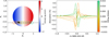 |
Fig. C.1 Orbital configuration, spot position, and corresponding absorption spectra for the sodium D1 line. Left panel: The planetary track is represented by a dashed line, with each open circle corresponding to an absorption spectrum of the same color, highlighting the local distortion. The colormap, ranging from blue to red, represents local velocities. Right panel: Evolution of the absorption spectrum as a function of the orbital phase. The spot-crossing effect induces a slight asymmetry that is visible in the local profiles in the stellar rest frame. |
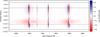 |
Fig. C.2 The time-series of absorption spectra around the sodium lines for the spot-crossing scenario is shown. The image covers a wavelength interval of 12 Å, centered on the mean position between the two lines. Horizontal black lines indicate the transit contacts: solid black represents T1 and T4, while dashed black denotes T2 and T3 (from negative to positive phase values). At phases corresponding to the spot position, an extra distortion is observed due to the spectral difference between the AR and the stellar photosphere. The sodium lines in the AR appear broader than those in the photosphere, resulting in an apparent emission that extends beyond the distortion near the line core. |
Solar-analog and Jupiter-analog system properties.
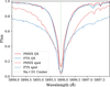 |
Fig. C.3 Comparison of the input spectra for the spot-crossing simulation. The figure presents the line profiles of Na I D1 line from observed spectra obtained with FTS-QS and FTS-spot. These include a quiet Sun observation at disk center (Wallace et al. 1998), shown as solid blue lines, and a sunspot umbral region (Wallace et al. 2005), represented by dashed blue lines. For comparison, we also display PHNX spectra, including the spectrum with the properties of a solar analog for the quiet Sun (solid red) and the spectrum of a star with a temperature 663 K lower than the Sun, representing the active region (dashed red). |
Appendix D HD 209458 Doppler shadow
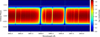 |
Fig. D.1 The time evolution of the stellar spectra occulted by the planet as a function of orbital phase, in the wavelength range 5882-5902 Å, which includes the sodium doublet. The positions of the Na I lines are highlighted by vertical dotted lines. The horizontal white lines indicate the transit contacts, with solid white representing T1 and T4, and dashed gray representing T2 and T3 (from negative to positive values of phase). This map was constructed by subtracting the in-transit flux-weighted spectra from a reference out-of-transit spectrum. |
Appendix E Comparison with S0AP2.0
The version of SOAP implemented in this paper is entirely written in Python, with the most critical and frequently executed parts compiled using Numba (Lam et al. 2015), a just-in-time compiler for Python. In this section, we compare the activity impact at the CCF level, as described in Dumusque et al. (2014), for both a spot and a facula by analyzing the integrated CCF results obtained with the original C code. For these simulations, we set a 1% filling factor region with a temperature contrast of 664 K for the spot and 250.9 K for the facula, following the contrast prescribed by Meunier et al. (2010). The active regions are positioned at the disk center, and the simulation evolves over one rotation period of the star, which has the same properties as those listed in Table C.1.
A comparison of the two versions, along with the residuals, is shown in Fig. E.1 for a spot and Fig. E.2 for a facula. The variation induced by equatorial spots and faculae agrees well, although residuals at the cm s-1 level are present.
The differences between the current model and the previous one primarily stem from two factors: an enhanced interpolation algorithm for CCF shifts during the construction of the stellar and AR signals, and a more refined method for selecting pixels in the grid. In the previous model, the interpolation process was carried out in two steps: first, the integer-pixel shift of the CCF was determined, and second, a first-order finite difference approximation was applied to the fractional remainder. This approach has now been replaced with a linear piecewise interpolation method, which offers improved performance, particularly for larger velocity shifts of the fractional remainder. Regarding pixel selection, the previous version relied on the pixel boundaries, whereas the current model uses the centroid of each pixel. This change enhances the stability of the grid, particularly when selecting an even or odd number of grid points. Additionally, the stability of the total number of pixels for each element in the simulation is improved, as it remains more consistent over the evolution of the simulation.
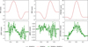 |
Fig. E.1 Variation in RV, bisector inverse slope (BIS), and full width at half maximum (FWHM) as a function of stellar rotation phase for an equatorial stellar spot with a filling factor of 1% and a temperature contrast of 663 K below the photosphere. Top: Comparison of the crosscorrelation function (CCF) properties simulated using S0AP2.0 and SOAPv4. Bottom: Difference between the simulations obtained with SOAPv4 and S0AP2.0. |
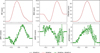 |
Fig. E.2 Same CCF properties and descriptions as in Fig. E.1, but for a facula with a temperature contrast of 250.9 K at the limb relative to the quiet photosphere. |
This amplitude represents a value that is unbinned in time and that decreases to ~40 cm s-1 with a realistic cadence (Meunier et al. 2015; Sulis et al. 2020), at which point supergranulation contributes comparably (Meunier & Lagrange 2020; Al Moulla et al. 2023).
This phenomenon is commonly, though inaccurately, referred to in the literature as the Rossiter-McLaughlin effect.
The code is publicly available on : https://github.com/EduardoCristo/SOAP-Spot-Oscillation-And-Planet-code
A CCF can be interpreted as a representation of the average line profile within a given spectral region.
A note on terminology: in some previous works, the term “plages” was used instead of “faculae”. While these terms are sometimes used interchangeably in the planetary community, in this code, we specifically simulate photospheric regions that are usually associated with faculae and not their chromospheric counterparts (e.g., Priest 1982; Basri 2021).
Granulation introduces distortions in line profiles that vary across the stellar disk. In observed spectra such as those from the IAG solar atlas, these effects are at least partially imprinted on the data, including line asymmetries and a component of the convective blueshift. While these spectra capture the average impact of granulation, however, they do not account for its temporal variability, that is, the changes in the RV that are induced by evolving granular patterns.
The spectral library is available at: https://www.astro.physik.uni-goettingen.de/research/solar-lib/
This normalization can be performed at any reference wavelength when the relative contrast is preserved and the wavelength is provided to the code.
In particular, the local continuum slope is lost, which primarily affects broader spectral regions, but its effect remains negligible for smaller wavelength bins.
The absorption spectrum A(λ) is defined as the ratio of the in-transit integrated spectrum to the mean out-of-transit spectrum. It is related with the transmission through the relation T(λ, t) = 1 − A(λ, t), where T(λ) represents the transmission spectrum. This formulation quantifies the fraction of stellar light that is absorbed by the planetary disk and exoplanet atmosphere as a function of wavelength and provides insight into its composition and structure.
The granulation signal imprinted on the observed spectra.
The resolution of the FTS observations is R>700 000, and that of the PHNX spectra is R=500 000.
All Tables
All Figures
|
Fig. 1 Depiction of the SOAP projection of a stellar disk onto a grid of 20 × 20 pixels for illustration purposes. The color map represents the local normalized flux in each position, which is determined by the limb-darkening. The white circumference outlines the original disk for reference. |
| In the text | |
|
Fig. 2 Position of a spot with a radius of 15% of the stellar radius at a latitude and longitude of 45° and projected onto a 300 × 300 pixel grid. The vertical and horizontal green lines indicate the precomputed bounding box that marks the minimum and maximum Cartesian coordinates within the grid. The brown points represent the calculated positions that define the spot boundary in its final projected location. |
| In the text | |
|
Fig. 3 Local line profiles centered on the sodium D2 line at different limb angles for a solar-like star that rotates as a solid body at 20 km s-1. The representation illustrates velocity variations from the disk center to the eastern limb for a star rotating from west to east. As the pixels approach the limb, the flux decreases due to limb darkening, while the projected velocity component increases. |
| In the text | |
|
Fig. 4 Variation in the sodium doublet line properties as a function of temperature contrast in regard to the solar case. Positive contrasts correspond to spectra of faculae, and negative contrasts represent spectra of spots. The quiet-star spectrum is indicated by the dashed white line at the zero level. All spectra used to construct the figure were taken from the PHOENIX library. |
| In the text | |
|
Fig. 5 IAG Na I D2 (top) and Na I D1 (bottom) Na I lines as a function of limb position. The wavelength interval was selected to represent a 3 Å region surrounding each line. Contaminated regions that are affected by neighboring lines were excluded, as demonstrated by the comparison with the integrated star spectrum shown in black. |
| In the text | |
|
Fig. 6 Comparison of the absorption spectra generated using SOAPv4 for a solar analog hosting a hot Jupiter. The top panel presents a comparison of the absorption profiles obtained using input spectra from IAG, TS, and PHNX spectra that matched the stellar properties. The bottom panel illustrates the differences between the absorption spectrum produced with IAG and the spectra derived from the other models. These simulations represent the POLDs centered on the Na I D1 line and span a wavelength range of 1 Å on either side. |
| In the text | |
|
Fig. 7 Top panel: full absorption profiles for the PHNX (blue) and FTS (red) input spectra without active regions (solid lines), together with the corresponding profiles with a stellar spot (dashed lines). Bottom panel: differential signals obtained by subtracting the quiet-star profiles from the spot-crossing profiles. The color-coding matches the input spectra. The wavelength interval is the same as in Fig. 6. |
| In the text | |
|
Fig. 8 Comparison of partial mean absorption spectra for QS and spotcrossing events. In the top panel, the profiles for the two scenarios are presented. The leading hemisphere profiles (blueshifted) are represented in blue and the trailing hemisphere profiles (redshifted) are shown in red. The bottom panel shows the difference between the partial profiles for the quiet-star and spot-crossing events. The same wavelength interval as in Fig. 6 is used. |
| In the text | |
|
Fig. 9 Absorption profiles of the Na I D lines in HD 20945 8 compared against the observed absorption profile derived from ESPRESSO data, as presented in Casasayas-Barris et al. (2021). In the top row, the absorption points are shown in black, and their respective uncertainties are represented by a confidence interval (CI in the plot) band at the 1σ level. The absorption features computed using SOAPv4 are overplotted. They were based on input MARCS models with two Na I abundances (solar-like) reported in the literature. The subsequent rows display the residuals between the models and observations. The colors of the data points and CI bands correspond to the respective model color. |
| In the text | |
|
Fig. 10 RV curves computed using SOAPv4 for an equatorial spot with a 1% filling factor, which is 663 K cooler than the photosphere. The color bar represents the average wavelength of the spectral bins, from which the radial velocities were derived using the CCF technique with the QS solar PHNX model. |
| In the text | |
|
Fig. C.1 Orbital configuration, spot position, and corresponding absorption spectra for the sodium D1 line. Left panel: The planetary track is represented by a dashed line, with each open circle corresponding to an absorption spectrum of the same color, highlighting the local distortion. The colormap, ranging from blue to red, represents local velocities. Right panel: Evolution of the absorption spectrum as a function of the orbital phase. The spot-crossing effect induces a slight asymmetry that is visible in the local profiles in the stellar rest frame. |
| In the text | |
|
Fig. C.2 The time-series of absorption spectra around the sodium lines for the spot-crossing scenario is shown. The image covers a wavelength interval of 12 Å, centered on the mean position between the two lines. Horizontal black lines indicate the transit contacts: solid black represents T1 and T4, while dashed black denotes T2 and T3 (from negative to positive phase values). At phases corresponding to the spot position, an extra distortion is observed due to the spectral difference between the AR and the stellar photosphere. The sodium lines in the AR appear broader than those in the photosphere, resulting in an apparent emission that extends beyond the distortion near the line core. |
| In the text | |
|
Fig. C.3 Comparison of the input spectra for the spot-crossing simulation. The figure presents the line profiles of Na I D1 line from observed spectra obtained with FTS-QS and FTS-spot. These include a quiet Sun observation at disk center (Wallace et al. 1998), shown as solid blue lines, and a sunspot umbral region (Wallace et al. 2005), represented by dashed blue lines. For comparison, we also display PHNX spectra, including the spectrum with the properties of a solar analog for the quiet Sun (solid red) and the spectrum of a star with a temperature 663 K lower than the Sun, representing the active region (dashed red). |
| In the text | |
|
Fig. D.1 The time evolution of the stellar spectra occulted by the planet as a function of orbital phase, in the wavelength range 5882-5902 Å, which includes the sodium doublet. The positions of the Na I lines are highlighted by vertical dotted lines. The horizontal white lines indicate the transit contacts, with solid white representing T1 and T4, and dashed gray representing T2 and T3 (from negative to positive values of phase). This map was constructed by subtracting the in-transit flux-weighted spectra from a reference out-of-transit spectrum. |
| In the text | |
|
Fig. E.1 Variation in RV, bisector inverse slope (BIS), and full width at half maximum (FWHM) as a function of stellar rotation phase for an equatorial stellar spot with a filling factor of 1% and a temperature contrast of 663 K below the photosphere. Top: Comparison of the crosscorrelation function (CCF) properties simulated using S0AP2.0 and SOAPv4. Bottom: Difference between the simulations obtained with SOAPv4 and S0AP2.0. |
| In the text | |
|
Fig. E.2 Same CCF properties and descriptions as in Fig. E.1, but for a facula with a temperature contrast of 250.9 K at the limb relative to the quiet photosphere. |
| In the text | |
Current usage metrics show cumulative count of Article Views (full-text article views including HTML views, PDF and ePub downloads, according to the available data) and Abstracts Views on Vision4Press platform.
Data correspond to usage on the plateform after 2015. The current usage metrics is available 48-96 hours after online publication and is updated daily on week days.
Initial download of the metrics may take a while.