© The Authors 2025

1. Introduction

Primordial non-Gaussianity (PNG) is the field of study of deviations from Gaussianity of primordial cosmological fluctuations. A wealth of information is expected to be encoded in the non-Gaussianity of the fluctuations, in particular regarding the period of the production of these fluctuations, most generally expected to be a model of inflation (see e.g., the reviews Bartolo et al. 2004; Chen 2010; Wang 2014; Renaux-Petel 2015; Achúcarro et al. 2022). For example, the size (parametrized by the so-called f_NL parameters) and type of non-Gaussianity, once detected, should allow us to distinguish between inflation models with multiple fields (see e.g., Vernizzi & Wands 2006; Rigopoulos et al. 2007; Byrnes & Choi 2010; Jung & van Tent 2017; de Putter et al. 2017; Wang et al. 2023), models with nonstandard kinetic terms (see e.g., Seery & Lidsey 2005; Chen et al. 2007; Bartolo et al. 2010), or the standard single-field slow-roll models of inflation (Maldacena 2003). Primordial non-Gaussianity can also put constraints on other models of the early Universe than inflation (see e.g., Lehners 2010; Agullo et al. 2018; van Tent et al. 2023). Together with the tensor-to-scalar ratio, PNG is the main primordial observable that we hope to measure in the future. The tensor-to-scalar ratio will tell us the energy scale at which inflation occurred and, together with the already observed amplitude and spectral index (slope) of the scalar power spectrum, allow us to also determine the first and second derivatives of the inflaton potential at that scale, at least for single-field slow-roll models (see e.g., Baumann 2011, for a review of inflation theory). However, as is indicated above, non-Gaussianity contains much more information for distinguishing between inflation models and, contrary to the tensor-to-scalar ratio, which could be arbitrarily small and hence unobservable, it has an explicit lower limit that is the prediction of single-field slow-roll inflation (Maldacena 2003) (although that limit is about two orders of magnitude smaller than what we can hope to measure with the CMB alone). In addition, PNG could show the presence of new massive particles in the context of the so-called cosmological collider (Arkani-Hamed & Maldacena 2015).

It is hence no wonder that PNG has been an important focus of cosmological surveys, mainly the cosmic microwave background (CMB) satellite missions of the past, WMAP (see e.g., Komatsu 2011; Bennett 2013) and Planck, and that it remains so for future missions such as LiteBIRD (Allys et al. 2023) (see also e.g., Finelli 2018). In particular, the Planck collaboration dedicated a full publication to PNG at each of its three official releases (PR1, PR2, and PR3), Planck Collaboration XXIV (2014), Planck Collaboration XVII (2016), Planck Collaboration IX (2020). The third of these had the most stringent observational constraints to date on a large number of types of non-Gaussianity. A similar level of constraints should in principle be reached or even improved upon with the new generation of galaxy surveys such as Euclid (Euclid Collaboration: Laureijs et al. 2011) (see e.g., Karagiannis et al. 2018), but they are not yet competitive with the CMB results (see D’Amico et al. 2025; Cabass et al. 2022a,b; Ivanov et al. 2024; Cagliari et al. 2025, for constraints based on the BOSS data). To determine the CMB bispectrum (the Fourier or spherical harmonic transform of the three-point correlator), which is the object statistical quantity where one generically expects the strongest PNG signal and the exclusive focus of this paper, three main estimators were used in the Planck papers: the Komatsu-Spergel-Wandelt (KSW) estimator (Komatsu et al. 2005; Yadav et al. 2007, 2008), the binned estimator (Bucher et al. 2010, 2016), and the modal estimator (Fergusson et al. 2010, 2012; Fergusson 2014)¹.

After the third Planck release, a part of the collaboration continued to work on the data-processing pipeline, creating a new one called NPIPE, which led to a final release, PR4 (Planck Collaboration LVII 2020). However, this release of data products was not accompanied by the usual suite of analysis papers. The cosmological parameters determined from the power spectra of PR4 were later published in Tristram (2024). However, no non-Gaussian analysis had been performed on the PR4 data so far². In addition to including previously neglected data from the repointing periods, NPIPE processed all the Planck channels within the same framework, including the latest versions of corrections for systematics and data treatment. This implies lower noise levels and reduced systematics in PR4 compared to PR3.

In this work, we perform the first bispectrum analysis of the PR4 data. We use both the effectively optimal (meaning optimal given the error bars) binned bispectrum estimator that was also used for all previous Planck releases, and an additional estimator that was developed later: the integrated bispectrum estimator (Jung et al. 2020). The integrated bispectrum estimator is nonoptimal and has only been developed for temperature, but it is very fast and allows us to cross-check results and do additional tests. We analyze the standard primordial (local, equilateral, and orthogonal) and secondary (lensing, unclustered point sources, and CIB) bispectrum shapes. We perform various validation tests and in particular analyze very carefully the 600 CMB and noise simulations that are used both for the linear correction term and for the error bars.

The outline of the paper is as follows. In Section 2, we define the CMB bispectrum and in particular its binned and integrated approximations. In Section 3, we recall the theoretical templates that we test for and the expression of the f_NL estimators. In Section 4, we describe the data and simulations we use. The main results of our paper are given in Section 5, followed by Section 6 with validation tests to confirm their robustness. We conclude in Section 7.

2. The CMB bispectrum

2.1. Definitions

To study small deviations from Gaussianity in the CMB, a key observable is the angle-averaged bispectrum defined by

$$\begin{array}{c}\hfill B_{{\ell }_1{\ell }_2{\ell }_3}^{p_1{p}_2{p}_3}\equiv \langle {\displaystyle {\int }_{S^2}}\mathrm{d}\widehat{\mathrm{\Omega }}{M}_{{\ell }_1}^{p_1}(\widehat{\mathrm{\Omega }})M_{{\ell }_2}^{p_2}(\widehat{\mathrm{\Omega }})M_{{\ell }_3}^{p_3}(\widehat{\mathrm{\Omega }})\rangle ,\end{array}$$(1)

where maps of the CMB temperature or E-polarization field denoted by the label p are filtered using the standard decomposition into spherical harmonics:

$$\begin{array}{c}\hfill M_{\ell }^p(\widehat{\mathrm{\Omega }})={\displaystyle \sum _{m=-\ell }^{+\ell }}{a}_{\ell m}^p{Y}_{\ell m}(\widehat{\mathrm{\Omega }}).\end{array}$$(2)

One can show that this angle-averaged bispectrum is related to the full angular bispectrum, which is defined as the three-point correlator of the harmonic coefficients, under the assumption of statistical isotropy by

$$\begin{array}{c}\hfill B_{{\ell }_1{\ell }_2{\ell }_3}=h_{{\ell }_1{\ell }_2{\ell }_3}{\displaystyle \sum _{m_1,m_2,m_3}}\left(\begin{array}{ccc}{\ell }_1& {\ell }_2& {\ell }_3\\ m_1& m_2& m_3\end{array}\right)⟨a_{{\ell }_1{m}_1}{a}_{{\ell }_2{m}_2}{a}_{{\ell }_3{m}_3}⟩,\end{array}$$(3)

where

$$\begin{array}{c}\hfill h_{{\ell }_1{\ell }_2{\ell }_3}=\sqrt{\frac{(2{\ell }_1+1)(2{\ell }_2+1)(2{\ell }_3+1)}{4\pi }}\left(\begin{array}{ccc}{\ell }_1& {\ell }_2& {\ell }_3\\ 0& 0& 0\end{array}\right).\end{array}$$(4)

Due to the presence of the 3j Wigner symbol in h_ℓ1ℓ2ℓ3, we need to consider only ℓ-triplets that fulfill both the parity condition (ℓ₁ + ℓ₂ + ℓ₃ even) and the triangle inequality (|ℓ₁ − ℓ₂|≤ℓ₃ ≤ ℓ₁ + ℓ₂).

Assuming weak non-Gaussianity, the bispectrum covariance matrix in polarization space becomes

$$\begin{array}{c}\hfill \mathrm{Covar}(B_{{\ell }_1{\ell }_2{\ell }_3}^{p_1{p}_2{p}_3},B_{{\ell }_1{\ell }_2{\ell }_3}^{p_4{p}_5{p}_6})=g_{{\ell }_1{\ell }_2{\ell }_3}{h}_{{\ell }_1{\ell }_2{\ell }_3}^2{C}_{{\ell }_1}^{p_1{p}_4}{C}_{{\ell }_2}^{p_2{p}_5}{C}_{{\ell }_3}^{p_3{p}_6},\end{array}$$(5)

where the factor g_ℓ1ℓ2ℓ3 is 6 when the three ℓs are the same, 2 when only two are equal, and 1 otherwise.

In practice, measuring the bispectrum for all configurations is computationally prohibitive. To address this challenge, several approaches have been developed, including the binned bispectrum and integrated bispectrum estimators, which we discuss in the following.

2.2. Binned bispectrum

The binned bispectrum method simply consists of using a binning of the multipole ℓ space to drastically reduce the number of mode triplets. It is well adapted to work with relatively smooth functions in harmonic space, which is the case of the different standard bispectrum templates we discuss later in Sect. 3.1. The binned bispectrum estimator and its implementation are described in Bucher et al. (2016) (see also Bucher et al. 2010; Jung et al. 2018, for details).

The binned bispectrum estimator can be written as

$$\begin{array}{c}\hfill {\widehat{B}}_{i_1{i}_2{i}_3}^{p_1{p}_2{p}_3}={\displaystyle {\int }_{S^2}}\mathrm{d}\widehat{\mathrm{\Omega }}{M}_{i_1}^{p_1}(\widehat{\mathrm{\Omega }})M_{i_2}^{p_2}(\widehat{\mathrm{\Omega }})M_{i_3}^{p_3}(\widehat{\mathrm{\Omega }})-B_{i_1{i}_2{i}_3}^{p_1{p}_2{p}_3,\mathrm{lin}},\end{array}$$(6)

where maps filtered over the i-th bin, denoted as Δ_i, are simply obtained using

$$\begin{array}{c}\hfill M_i^p(\widehat{\mathrm{\Omega }})={\displaystyle \sum _{\ell \in {\mathrm{\Delta }}_i}}{M}_{\ell }^p(\widehat{\mathrm{\Omega }}).\end{array}$$(7)

The linear correction term B_i1i2i3^{p₁p₂p₃, lin} is necessary to maintain the optimality of the estimator when features breaking the expected isotropy of the signal have to be taken into account. For example, with observational datasets, masking some regions of the sky such as the galactic plane, as well as the anisotropic scanning pattern of the mission that leads to anisotropic noise levels, has such an effect. This correction was computed using

$$\begin{array}{cc}\hfill B_{i_1{i}_2{i}_3}^{p_1{p}_2{p}_3,\mathrm{lin}}={\displaystyle {\int }_{S^2}}\mathrm{d}\widehat{\mathrm{\Omega }}[& M_{i_1}^{p_1}\langle M_{i_2}^{p_2}{M}_{i_3}^{p_3}\rangle \hfill \\ \hfill & +M_{i_2}^{p_2}\langle M_{i_1}^{p_1}{M}_{i_3}^{p_3}\rangle +M_{i_3}^{p_3}\langle M_{i_1}^{p_1}{M}_{i_2}^{p_2}\rangle ],\hfill \end{array}$$(8)

where the ensemble averages were calculated over CMB simulations with the same characteristics as the observations (beam, noise, and mask). Moreover, the estimated binned bispectrum should be multiplied by the factor 1/f_sky, with f_sky the unmasked fraction of the sky, before any comparison to full-sky theoretical predictions.

From a known theoretical bispectrum template (see Sect. 3.1 for examples), it is straightforward to compute the corresponding theoretical binned bispectrum,

$$\begin{array}{c}\hfill B_{i_1{i}_2{i}_3}^{p_1{p}_2{p}_3,\mathrm{th}}={\displaystyle \sum _{{\ell }_1\in {\mathrm{\Delta }}_1}}{\displaystyle \sum _{{\ell }_2\in {\mathrm{\Delta }}_2}}{\displaystyle \sum _{{\ell }_3\in {\mathrm{\Delta }}_3}}{B}_{{\ell }_1{\ell }_2{\ell }_3}^{p_1{p}_2{p}_3,\mathrm{th}}.\end{array}$$(9)

The covariance matrix of the binned bispectrum in polarization space is given by

$$\begin{array}{cc}\hfill \mathrm{Covar}(B_{i_1{i}_2{i}_3}^{p_1{p}_2{p}_3},B_{i_1{i}_2{i}_3}^{p_4{p}_5{p}_6})& \equiv V_{i_1{i}_2{i}_3}^{p_1{p}_2{p}_3{p}_4{p}_5{p}_6}\hfill \\ \hfill & =g_{i_1{i}_2{i}_3}\hfill \\ \hfill & \times {\displaystyle \sum _{{\ell }_1\in {\mathrm{\Delta }}_1}}{\displaystyle \sum _{{\ell }_2\in {\mathrm{\Delta }}_2}}{\displaystyle \sum _{{\ell }_3\in {\mathrm{\Delta }}_3}}{h}_{{\ell }_1{\ell }_2{\ell }_3}^2{C}_{{\ell }_1}^{p_1{p}_4}{C}_{{\ell }_2}^{p_2{p}_5}{C}_{{\ell }_3}^{p_3{p}_6}.\hfill \end{array}$$(10)

To take into account instrumental effects, one has to apply the following modifications to Eqs. (9) and (10):

$$\begin{array}{c}\hfill C_{\ell }\to b_{\ell }^2{C}_{\ell }+N_{\ell },B_{{\ell }_1{\ell }_2{\ell }_3}\to b_{{\ell }_1}{b}_{{\ell }_2}{b}_{{\ell }_3}{B}_{{\ell }_1{\ell }_2{\ell }_3},\end{array}$$(11)

where b_ℓ is the beam window function and N_ℓ the noise power spectrum.

2.3. Integrated bispectrum

The integrated bispectrum method follows a different and simpler approach to extract the relevant bispectral information. Based on the original idea of Chiang et al. (2014), developed in the context of large-scale structure studies, it consists of dividing the sky into many equal-size patches and computing the average correlation of the mean value and the power spectrum in each patch. We adopted the same methodology as in Jung et al. (2020), recalling here only the key steps.

The full integrated bispectrum estimator can be written as

$$\begin{array}{c}\hfill {\widehat{\mathrm{I}B}}_{\ell }=\frac{1}{N_{\mathrm{patch}}}{\displaystyle \sum _{\mathrm{patch}}}{\overline{M}}^{\mathrm{patch}}{C}_{\ell }^{\mathrm{patch}}-\mathrm{I}{B}_{\ell }^{\mathrm{lin}},\end{array}$$(12)

where ${\overline{M}}^{\mathrm{patch}}$ and C_ℓ^patch are, respectively, the measured mean value and power spectrum in a given patch, and N_patch is the total number of patches. Note that in this expression, we dropped the p subscript, as we only consider temperature maps with the integrated bispectrum estimator in this work. Similarly to the binned bispectrum case, the linear correction term I​B_ℓ^lin was used to maintain optimality when anisotropy breaking effects (mask, anisotropic noise) are present in the data. It took the form

$$\begin{array}{c}\hfill \mathrm{I}{B}_{\ell }^{\mathrm{lin}}=\frac{1}{N_{\mathrm{patch}}}{\displaystyle \sum _{\mathrm{patch}}}{\overline{M}}^{\mathrm{patch}}{C}_{\ell }^{\mathrm{patch},\mathrm{sims}},\end{array}$$(13)

where the C_ℓ^{patch, sims} were evaluated from a sufficiently large set of simulations reproducing the main characteristics of observations (e.g., mask, noise, and beam). Additionally, the estimated integrated bispectrum was multiplied by the factor 1/f_sky if the sky was partially masked.

One can directly relate the theoretical expectation of the integrated bispectrum and the theoretical bispectrum template, and the expression only depends on the shape, size, and position of the patches. In the case of azimuthally symmetric patches, this link is given by

$$\begin{array}{c}\hfill \mathrm{I}{B}_{\ell }^{\mathrm{th}}=\frac{1}{{(4\pi )}^3}{\displaystyle \sum _{{\ell }_1{\ell }_2{\ell }_3{\ell }_4{\ell }_5}}{w}_{{\ell }_3}{w}_{{\ell }_4}{w}_{{\ell }_5}{\mathcal{F}}_{\ell {\ell }_1{\ell }_2{\ell }_3{\ell }_4{\ell }_5}{B}_{{\ell }_1{\ell }_2{\ell }_3}^{\mathrm{th}},\\ \hfill \end{array}$$(14)

where the factor

$$\begin{array}{cc}& {\mathcal{F}}_{\ell {\ell }_1{\ell }_2{\ell }_3{\ell }_4{\ell }_5}\equiv {(-1)}^{{\ell }_2+{\ell }_4}(2{\ell }_4+1)(2{\ell }_5+1){\left(\begin{array}{ccc}{\ell }_1& {\ell }_2& {\ell }_3\\ 0& 0& 0\end{array}\right)}^{-1}\hfill \\ & \times \left(\begin{array}{ccc}\ell & {\ell }_1& {\ell }_4\\ 0& 0& 0\end{array}\right)\left(\begin{array}{ccc}\ell & {\ell }_2& {\ell }_5\\ 0& 0& 0\end{array}\right)\left(\begin{array}{ccc}{\ell }_3& {\ell }_4& {\ell }_5\\ 0& 0& 0\end{array}\right)\left\{\begin{array}{ccc}{\ell }_1& {\ell }_2& {\ell }_3\\ {\ell }_5& {\ell }_4& \ell \end{array}\right\}\hfill \end{array}$$(15)

only depends on Wigner 3j and 6j symbols (in parentheses and braces, respectively), and w_ℓ is a simple function in harmonic space that defines the full set of patches³. In this work, we used the same set of patches as in Jung et al. (2020) defined by w_ℓ = 1 for ℓ ≤ 10 and 0 otherwise. This implies that we probed only the squeezed limit of the bispectrum.

The covariance of the integrated bispectrum can be computed in a similar manner using the weakly non-Gaussian approximation and Eq. (5):

$$\begin{array}{cc}\hfill {\mathrm{IC}}_{\ell \ell \prime }& \equiv \mathrm{Covar}(\mathrm{I}{B}_{\ell },\mathrm{I}{B}_{\ell \prime })\hfill \\ \hfill & =\frac{1}{{(4\pi )}^6}{\displaystyle \sum _{{\ell }_1{\ell }_2{\ell }_3{\ell }_4{\ell }_5\ell {\prime }_4\ell {\prime }_5}}{h}_{{\ell }_1{\ell }_2{\ell }_3}^2{\mathcal{F}}_{\ell {\ell }_1{\ell }_2{\ell }_3{\ell }_4{\ell }_5}{w}_{{\ell }_3}{w}_{{\ell }_4}{w}_{{\ell }_5}{w}_{\ell {\prime }_4}{w}_{\ell {\prime }_5}{C}_{{\ell }_1}{C}_{{\ell }_2}{C}_{{\ell }_3}\hfill \\ \hfill & \times [w_{{\ell }_3}({\mathcal{F}}_{\ell \prime {\ell }_1{\ell }_2{\ell }_3\ell {\prime }_4\ell {\prime }_5}+{\mathcal{F}}_{\ell \prime {\ell }_2{\ell }_1{\ell }_3\ell {\prime }_4\ell {\prime }_5})\hfill \\ \hfill & +w_{{\ell }_2}({\mathcal{F}}_{\ell \prime {\ell }_1{\ell }_3{\ell }_2\ell {\prime }_4\ell {\prime }_5}+{\mathcal{F}}_{\ell \prime {\ell }_3{\ell }_1{\ell }_2\ell {\prime }_4\ell {\prime }_5})\hfill \\ \hfill & +w_{{\ell }_1}({\mathcal{F}}_{\ell \prime {\ell }_3{\ell }_2{\ell }_1\ell {\prime }_4\ell {\prime }_5}+{\mathcal{F}}_{\ell \prime {\ell }_2{\ell }_3{\ell }_1\ell {\prime }_4\ell {\prime }_5})].\hfill \end{array}$$(16)

In the realistic case, the same modifications as for the binned bispectrum (Eq. (11)) should be applied to Eqs. (14) and (16).

3. Parametric estimation

3.1. Theoretical shapes

The presence of a small amount of PNG is a prediction of many different inflationary models beyond the standard single-field slow-roll scenario. These models produce distinct bispectrum shapes depending on their specific characteristics. Here, we focus on the local, equilateral, and orthogonal templates that were studied in detail in the Planck PNG analyses (Planck Collaboration XXIV 2014; Planck Collaboration XVII 2016; Planck Collaboration IX 2020).

These three bispectrum shapes can be written as functions of the primordial power spectrum of the gravitational potential, P(k) = A(k/k₀)^{n_s − 4}, where A is its amplitude, k₀ the pivot scale, and n_s the spectral index,

$$\begin{array}{cc}\hfill B^{\mathrm{local}}(k_1,k_2,k_3)& =2[P(k_1)P(k_2)+P(k_1)P(k_3)+P(k_2)P(k_3)],\hfill \\ \hfill B^{\mathrm{equil}}(k_1,k_2,k_3)& =-6[P(k_1)P(k_2)+(2perms)]\hfill \\ \hfill & -12P^{2/3}(k_1)P^{2/3}(k_2)P^{2/3}(k_3)\hfill \\ \hfill & +6[P(k_1)P^{2/3}(k_2)P^{1/3}(k_3)+(5perms)],\hfill \\ \hfill B^{\mathrm{ortho}}(k_1,k_2,k_3)& =-18[P(k_1)P(k_2)+(2perms)]\hfill \\ \hfill & -48P^{2/3}(k_1)P^{2/3}(k_2)P^{2/3}(k_3)\hfill \\ \hfill & +18[P(k_1)P^{2/3}(k_2)P^{1/3}(k_3)+(5perms)].\hfill \end{array}$$(17)

The local type of PNG (Gangui et al. 1994) is mostly related to multiple-field inflation, whereby curvature perturbations can evolve on superhorizon scales (see e.g., Rigopoulos et al. 2007; Byrnes & Choi 2010). The equilateral and orthogonal templates cover a wide range of inflationary models that have nonstandard kinetic terms or higher-derivative interactions (see e.g., Creminelli et al. 2006; Chen et al. 2007; Senatore et al. 2010).

The corresponding bispectra in the CMB anisotropies can then be computed using (Komatsu & Spergel 2001)

$$\begin{array}{cc}\hfill B_{{\ell }_1{\ell }_2{\ell }_3}^{p_1{p}_2{p}_3,\mathrm{th}}& =h_{{\ell }_1{\ell }_2{\ell }_3}^2{\left(\frac{2}{\pi }\right)}^3{\displaystyle {\int }_0^{\infty }}{k}_1^{2}d{k}_1{\displaystyle {\int }_0^{\infty }}{k}_2^{2}d{k}_2{\displaystyle {\int }_0^{\infty }}{k}_3^{2}d{k}_3\hfill \\ \hfill & [{\mathrm{\Delta }}_{{\ell }_1}^{p_1}(k_1){\mathrm{\Delta }}_{{\ell }_2}^{p_2}(k_2){\mathrm{\Delta }}_{{\ell }_3}^{p_3}(k_3)B(k_1,k_2,k_3)\hfill \\ \hfill & \times {\displaystyle {\int }_0^{\infty }}{r}^{2}dr{j}_{{\ell }_1}(k_{1}r)j_{{\ell }_2}(k_{2}r)j_{{\ell }_3}(k_{3}r)],\hfill \end{array}$$(18)

where ${\mathrm{\Delta }}_{\ell }^p(k)$ are the radiation transfer functions and j_ℓ are the spherical Bessel functions.

There are other sources of bispectral NG in the CMB due to the presence of different foregrounds. The contribution of the three main extragalactic⁴ ones, which are observable in the Planck data, can be taken into account using the following templates.

First, the bispectrum due to gravitational lensing (in temperature anisotropies caused by the correlation of the integrated Sachs-Wolfe (ISW) and lensing effects) (Hu 2000; Lewis et al. 2011) is

$$\begin{array}{c}\hfill B_{{\ell }_1{\ell }_2{\ell }_3}^{p_1{p}_2{p}_3,\mathrm{lens}}=h_{{\ell }_1{\ell }_2{\ell }_3}^2[f_{{\ell }_1{\ell }_2{\ell }_3}^{p_1}{C}_{{\ell }_2}^{p_2\varphi }{C}_{{\ell }_3}^{p_1{p}_3}+(5perms)],\end{array}$$(19)

where the C_ℓ^p₁p₂ are lensed power spectra and $C_{\ell }^{T\varphi }$ ($C_{\ell }^{E\varphi }$) is the temperature(polarization)-lensing cross-power spectrum. The f_ℓ1ℓ2ℓ3^p factors are given by

$$\begin{array}{cc}\hfill f_{{\ell }_1{\ell }_2{\ell }_3}^T& =\frac{1}{2}[{\ell }_2({\ell }_2+1)+{\ell }_3({\ell }_3+1)-{\ell }_1({\ell }_1+1)],\hfill \\ \hfill f_{{\ell }_1{\ell }_2{\ell }_3}^E& =\frac{1}{2}[{\ell }_2({\ell }_2+1)+{\ell }_3({\ell }_3+1)-{\ell }_1({\ell }_1+1)]\hfill \\ & \times \left(\begin{array}{ccc}{\ell }_1& {\ell }_2& {\ell }_3\\ 2& 0& -2\end{array}\right){\left(\begin{array}{ccc}{\ell }_1& {\ell }_2& {\ell }_3\\ 0& 0& 0\end{array}\right)}^{-1}.\hfill \end{array}$$(20)

The NG signature associated with unclustered point sources can be described by the simple shape (Komatsu & Spergel 2001)

$$\begin{array}{c}\hfill B_{{\ell }_1{\ell }_2{\ell }_3}^{\mathrm{ps}}=h_{{\ell }_1{\ell }_2{\ell }_3}^2,\end{array}$$(21)

while the cosmic infrared background (CIB) contribution is given by the heuristic template (Lacasa et al. 2014; Pénin et al. 2014)

$$\begin{array}{c}\hfill B_{{\ell }_1{\ell }_2{\ell }_3}^{\mathrm{CIB}}=h_{{\ell }_1{\ell }_2{\ell }_3}^2{\left[\frac{(1+{\ell }_1/{\ell }_{\mathrm{break}})(1+{\ell }_2/{\ell }_{\mathrm{break}})(1+{\ell }_3/{\ell }_{\mathrm{break}})}{{(1+{\ell }_0/{\ell }_{\mathrm{break}})}^3}\right]}^q,\end{array}$$(22)

where the break and pivot scales are ℓ_break = 70 and ℓ₀ = 320, respectively, and the index is q = 0.85.

3.2. Estimator

The optimal estimator of the amplitude parameter, f_NL, for a given bispectrum shape, B^th, determined from the observed bispectrum, $\widehat{B}$, is

$$\begin{array}{c}\hfill {\widehat{f}}_{\mathrm{NL}}=\frac{⟨\widehat{B},B^{\mathrm{th}}⟩}{⟨B^{\mathrm{th}},B^{\mathrm{th}}⟩},\end{array}$$(23)

where the exact definition of the inner product denoted as ⟨x, y⟩ depends on the bispectrum estimator used. For the binned and integrated bispectra, respectively, it is

$$\begin{array}{cc}\hfill {⟨B^a,B^b⟩}^{\mathrm{binned}}& \equiv {\displaystyle \sum _{i_1\le i_2\le i_3}}{\displaystyle \sum _{\begin{array}{c}{p}_1{p}_2{p}_3\\ p_4{p}_5{p}_6\end{array}}}{B}_{i_1{i}_2{i}_3}^{p_1{p}_2{p}_3,a}{\left(V^{-1}\right)}_{i_1{i}_2{i}_3}^{p_1{p}_2{p}_3{p}_4{p}_5{p}_6}{B}_{i_1{i}_2{i}_3}^{p_4{p}_5{p}_6,b},\hfill \\ \hfill {⟨B^a,B^b⟩}^{\mathrm{integrated}}& \equiv {\displaystyle \sum _{{\ell }_1{\ell }_2}}\mathrm{I}{B}_{{\ell }_1}^a{\left({\mathrm{IC}}^{-1}\right)}_{{\ell }_1{\ell }_2}\mathrm{I}{B}_{{\ell }_2}^b.\hfill \end{array}$$(24)

The expected variance of ${\widehat{f}}_{\mathrm{NL}}$ is given by 1/⟨B^th, B^th⟩, which has to be multiplied by 1/f_sky in the case of incomplete sky coverage.

Another important quantity is the bias f_NL^(1),(2) on the measurement of f_NL⁽¹⁾ for a given shape, B⁽¹⁾, due to the presence of another bispectrum, B⁽²⁾, of known amplitude f_NL⁽²⁾:

$$\begin{array}{c}\hfill f_{\mathrm{NL}}^{(1),(2)}=-\frac{F_{12}}{F_{11}}{f}_{\mathrm{NL}}^{(2)},\end{array}$$(25)

where the Fisher matrix elements are F_ab = ⟨B^a, B^b⟩. This is relevant to subtract the impact of the fully known lensing bispectrum (see Eq. (19); its f_NL is known to be unity) on the PNG estimation.

If the amplitude of the other shape(s) is not known, the correct approach is to perform a joint estimation of the different shapes of interest. In that case, the estimator defined in Eq. (23) becomes

$$\begin{array}{c}\hfill {\widehat{f}}_{\mathrm{NL}}^a={\displaystyle \sum _b}{(F^{-1})}_{\mathit{ab}}⟨\widehat{B},B^b⟩.\end{array}$$(26)

In this case, the expected variance of ${\widehat{f}}_{\mathrm{NL}}^a$ (also called Fisher error bars after taking a square root), which in the independent case can be written as 1/F_aa as indicated above, becomes for the joint analysis (F⁻¹)_aa.

4. Data and simulations

Our analyses are based on data and simulations from the latest Planck release (PR4) (see Planck Collaboration LVII 2020, for details). We used the temperature and polarization maps produced by the component separation technique SEVEM (Leach 2008; Fernandez-Cobos et al. 2012), which removes the large NG contamination due to several galactic foregrounds (see e.g., Jung et al. 2018; Coulton & Spergel 2019). These maps, which have a beam size of 5 arcminutes, are available on the Planck Legacy Archive⁵ (PLA). We also utilized the 600 corresponding CMB and noise simulations, which can be downloaded from the National Energy Research Scientific Computing Center⁶ (NERSC).

We used the 2018 Planck common mask (Planck Collaboration IV 2020), also available on the PLA, which leaves an observed fraction of the sky of f_sky = 0.779 and f_sky = 0.781 for temperature and polarization, respectively. After applying this mask to the different temperature and E-polarization map, the same standard diffusive inpainting technique as for previous Planck releases (Bucher et al. 2016; Gruetjen et al. 2017) was used to avoid spurious effects due to both the lack of small-scale power inside the mask and the edge discontinuity, both of which would leak into the unmasked region of the map during the filtering process in harmonic space.

For comparison purposes, we also considered the results obtained previously in Planck Collaboration IX (2020) and Jung et al. (2020) on the SEVEM maps (data and 300 simulations) from the previous release (PR3) (see Planck Collaboration IV 2020, for more information). The binned bispectrum estimator uses the same binning for the PR4 analysis as was used for PR3, and the integrated bispectrum estimator uses the same set of patches.

In Fig. 1, we show the temperature and E-polarization noise power spectra determined from the SEVEM PR3 and PR4 simulations, as well as the full CMB+noise power spectra. This confirms the lower level of noise in the PR4 data on a wide range of scales, allowing one to, for example, extract additional non-Gaussian information from small scales.

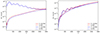Fig. 1. Full and noise-only power spectra determined from SEVEM PR3 and PR4 simulations, for temperature (left) and E-polarization (right).

5. Main results

In this section, we present our analysis of bispectral non-Gaussianity in the latest release of the Planck data. We updated the constraints on PNG of the previous Planck PNG analyses (Planck Collaboration XXIV 2014; Planck Collaboration XVII 2016; Planck Collaboration IX 2020) using a similar methodology. We studied the temperature and E-polarization CMB maps produced by the component separation technique SEVEM for the Planck 2020 data release (PR4, see Sect. 4). We utilized two different bispectrum estimators to cross-validate our findings, both introduced in Sect. 2. Our main results were obtained by applying to the full dataset the binned bispectrum estimator to investigate standard shapes of primordial origin, namely the local, equilateral, and orthogonal ones, and late-time NG in the form of lensing, CIB, and unclustered point sources (all described in Sect. 3.1). Additionally, we used the integrated bispectrum estimator to constrain the local and lensing bispectra, both of which peak in the squeezed limit, from the CMB temperature map alone.

In Table 1, we show our constraints on the PNG amplitudes, f_NL^local, f_NL^equil, and f_NL^ortho. These results can be compared to Table 5 of Planck Collaboration IX (2020) and Table 3 of Jung et al. (2020) for the binned and integrated bispectrum estimators, respectively. These values were obtained in independent estimations, with and without removing the bias due to the expected presence of the lensing bispectrum in the data using Eq. (25), and including scales up to ℓ_max = 2500. The more conservative approach of analyzing the lensing contribution jointly with the PNG shapes leads to similar conclusions with only slightly larger error bars, as can be seen in Table 2. As in the analyses conducted on data from the previous Planck releases, the three considered f_NL parameters are fully compatible with zero in all cases.

Table 3 summarizes our results for the bispectrum amplitudes from late-time NG, to be compared to Tables 1 and 4 of Planck Collaboration IX (2020). As was known from previous analyses, the lensing bispectrum is detected at a value rather low but compatible with the expected amplitude of 1. As the detected value is extremely close to the Planck 2018 result, we recall that in Planck Collaboration IX (2020) it was pointed out that performing the same analysis on maps where the thermal Sunayev-Zeldovich (tSZ) signal has been removed in addition to the galactic foreground contribution increases the measured lensing amplitude to a value much closer to 1. This is likely due to the correlations between the ISW and tSZ effects that produce another bispectrum, as was first shown by Hill (2018). These maps have not been produced for the PR4 release, which implies that we could not perform a similar analysis. However, it was verified by Jung et al. (2020) and Coulton et al. (2023) that the ISW-tSZ-tSZ bispectrum amplitude is too low at the Planck resolution to impact significantly our constraints on PNG; and we expect the same conclusion to hold here.

The unclustered point sources and CIB amplitudes, b_PS and b_CIB, respectively, were estimated jointly as these two shapes are highly correlated. The former is detected at a nearly 3σ level in the data. However, it is important to recall that, unlike the lensing bispectrum, this shape has a very low correlation with the various primordial templates, and therefore cannot contaminate the results presented in Table 1. The results for these two templates are only shown for temperature as the CIB is not expected to be polarized. As for unclustered point sources, no bispectral contribution is detected in polarization (Planck Collaboration IX 2020), and as the point sources in temperature and polarization are not necessarily the same, it does not make sense to perform a joint temperature-polarization analysis.

In Table 4, we illustrate the improvement in constraints achieved with the PR4 dataset compared to the PR3 results (using SEVEM for both). First, we show the expected refinement computed with a Fisher approach. This improvement ranges from a few percent up to 12% depending on the bispectrum shape and if temperature and/or polarization are considered. In the most constraining case, which is the binned bispectrum T + E analysis, smaller error bars (by 7, 4, and 8% for the local, equilateral, and orthogonal shapes, respectively, and 11% for lensing) are predicted. Second, we made the same comparison between error bars determined in the actual analyses using the binned bispectrum and integrated bispectrum estimators on the Planck PR4 and PR3 datasets. In most cases, they are very close to the Fisher forecast. For the binned bispectrum T + E analysis, the improvement is, however, slightly lower than expected for the local shape, and higher for the orthogonal and lensing shapes, with a difference of 4% each time. This small difference can be explained by the fact that the error bars themselves were determined with a relative error of 4.1% and 2.8% for PR3 and PR4⁷, respectively. Another important result to mention is that all estimator error bars are compatible with their Fisher predictions. Only for the lensing shape do we obtain results that are slightly suboptimal, with a smaller difference in the case of PR4 (15% in PR4 versus 21% in PR3 for the binned bispectrum T + E).

These different results confirm the tightening of the constraints on the NG amplitude parameters obtained from a bispectrum analysis of the Planck PR4 data. The improvement by a few percentage points for the primordial local, orthogonal, and equilateral constraints makes them the most stringent constraints on these parameters to date, without changing the main conclusions of the previous Planck PNG analysis based on the PR3 data (Planck Collaboration IX 2020).

6. Validation tests

To confirm the robustness of our data analysis results presented in Sect. 5, we applied the same pipelines to the Planck PR4 simulations. In Table 5, we show the amplitude parameters averaged over the 600 available simulations and their corresponding standard errors, for the primordial local, equilateral, and orthogonal templates, and the lensing shape.

We verified that the PNG f_NLs are consistent with the expected value of zero, as no PNG is included in the simulations. While there are small deviations from zero (of order1–1.5σ) in the T or E-only analyses for the local and equilateral shapes, they disappear in the binned T + E case, which provides the most stringent constraints. The situation is similar for the orthogonal shape, which, however, has a slightly stronger deviation (2.5σ) in the binned T-only analysis. Even if this turned out not to be a statistical fluctuation, this deviation is still one order of magnitude smaller than the error bar on one map, used for the constraints in Table 1, and thus cannot bias our results in any significant manner.

Concerning the lensing bispectrum, we find a significant deviation from the expected value of 1, with both estimators and in all cases (although the significance is lower for the binned E-only and integrated bispectrum analyses, due to much larger error bars). In the remainder of the section, we check several possible origins of this issue and verify that it has no impact on our constraints derived from the Planck PR4 data. However, we stress that this deviation, while statistically significant due to the averages computed from many simulations, remains small compared to the 1σ observational error bars and is therefore negligible with respect to the statistical fluctuations expected in the data maps.

We performed a series of tests to confirm that this issue is already present at the level of the original CMB simulations, and thus is not an artifact of either the Planck PR4 NPIPE pipeline or the SEVEM component separation technique. First, we made a direct comparison of the Planck PR3 and PR4 simulation results. For both releases, lensed CMB realizations have been produced and processed through different pipelines to reproduce as accurately as possible the different instrumental effects (see Planck Collaboration II 2020; Planck Collaboration III 2020; Planck Collaboration IV 2020 and Planck Collaboration LVII 2020 for details on PR3 and PR4, respectively). There is a common set of 100 CMB seeds fully processed for both releases (the ones numbered from 200 to 299 in the simulation sample).

In Table 6, we show the results obtained from the analysis of these 100 simulations for both PR3 and PR4 using the binned bispectrum estimator. Concerning the local, equilateral, and orthogonal shapes, the measured f_NL values are compatible with the expected absence of PNG in these simulations. The lensing bispectrum is measured with similar amplitudes for the T and T + E amplitudes in both sets close to a value of 0.9, a few standard deviations below the expected value of 1 (the E-polarization error bars are one order of magnitude larger, and thus not sufficient to detect any deviation of the same order).This means that the new processing of instrumental effects used in the PR4 simulations does not bias the lensing results, at least with respect to the PR3 results. Note that in this specific set of 100 simulations common to PR3 and PR4, most error bars are of the same order between the two releases. This is because 100 simulations are not sufficient to obtain fully converged numerical results that can show the small improvements obtained with PR4 that we highlighted in Sect. 5.

We also evaluated the impact of the cleaning technique SEVEM on the PNG results. We focused on the PR3 simulated maps, as more component separation methods were applied for that release. In Planck Collaboration IX (2020), the main reported results were based on the SMICA method (Cardoso et al. 2008). In Table 7 we verify that in the 300 available PR3 simulations, we obtain very similar results for both SEVEM and SMICA. By comparing Tables 6 and 7, we directly see that the results are extremely close to each other, at a level much better than the expected error bars. As the two cleaning procedures are based on very different methods, no correlation of possible biases is expected, and thus this indicates that neither the PNG nor the lensing bispectrum amplitudes are biased by SEVEM.

A further investigation of this small discrepancy between the measured lensing amplitude in the simulations and the expected value of 1 would require us to check in detail steps such as the lensing implementation in the CMB simulations based on LensPix (Lewis 2005) and the accuracy of the theoretical computation of the lensing bispectrum. This is, however, beyond the scope of the present work, and thus we focus here on assessing that this discrepancy does not have an impact on the reported observational constraints.

The binned and integrated bispectrum estimators explicitly reconstruct the bispectrum in addition to measuring amplitude parameters. This allows us to use the averaged bispectrum from the simulations as a theoretical template, to estimate how much it can bias the results from the observations. In Table 8, we show the f_NL parameters of the local, equilateral, and orthogonal shapes measured in the PR4 data, after subtracting the bias of the averaged simulation bispectrum. As can be verified by comparison to Table 1, these results are extremely close to the values obtained by removing the standard lensing theoretical bias, with deviations one order of magnitude smaller than the 1σ error bars. This confirms that even if there is a small discrepancy between the simulations and the expected theoretical predictions, it is too small to affect the reported observational constraints, at least as far as the central values are concerned.

We next checked the impact on the error bars. We focused on the local PNG shape, which is by far the most correlated with the lensing bispectrum as they both peak in the squeezed limit. We used the integrated bispectrum estimator with subsets of 100 simulations taken among the 600 available ones to compute both the linear correction term and the error bars (for temperature alone). We randomly drew many such subsets and measured the average lensing amplitude of the simulations, as well as the central value and error bar of f_NL^local. For all these sets, we show the corresponding values in Fig. 2. Although there is a variation in both f_NL^local and its error bar depending on the specific subset, the results confirm that it is uncorrelated with the lensing amplitude of the specific subset and that it is actually compatible with the differences expected from a random Gaussian field.

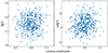Fig. 2. Estimated ${\widehat{f}}_{\mathrm{NL}}^{\mathrm{local}}$ (left) and its error bar $\sigma ({\widehat{f}}_{\mathrm{NL}}^{\mathrm{local}})$ (right) using different subsets of the PR4 simulations for linear correction and error bars, as a function of the lensing amplitude in the corresponding subset, determined using the integrated bispectrum estimator. Each subset consists of 100 maps drawn randomly from the 600 SEVEM PR4 simulations. Note that the expected lensing bias of 4.3 on the estimated ${\widehat{f}}_{\mathrm{NL}}^{\mathrm{local}}$ has not been subtracted.

7. Conclusions

In this work, we performed the first analysis of the standard non-Gaussian bispectrum templates on the Planck PR4 CMB data (Planck Collaboration LVII 2020), both temperature and E-polarization. These are the local, equilateral, and orthogonal primordial templates, and the secondary bispectrum templates for lensing, unclustered extragalactic point sources, and the CIB. The results of the full T + E analysis are f_NL^local = −0.1 ± 5.0, f_NL^equil = 6 ± 46, and f_NL^ortho = −8 ± 21. While the improvements in the error bars are only a few percentage points with respect to the PR3 results (up to 12% for orthogonal), these now stand as the best constraints on PNG from Planck. As the error bars were determined from 600 simulations instead of 300 for PR3, they should also be even more accurate. The results are fully consistent with the PR3 results and no primordial non-Gaussianity is detected.

The analysis in this paper is more limited than the one in the full Planck collaboration paper on PNG for PR3 (Planck Collaboration IX 2020). In the first place, this is due to the available maps: only the SEVEM component separation technique was applied to the PR4 maps to produce everything needed for a non-Gaussianity analysis. For PR3, four different component separation techniques were applied, including SMICA, which was chosen as the default method in all previous releases. In the second place, this is due to using only one effectively optimal bispectrum estimator, the binned bispectrum estimator, with support from the nonoptimal but very fast integrated bispectrum estimator for cross-checking certain results and running additional tests. For PR3, three different effectively optimal estimators (with four independent pipelines) were used, including the KSW estimator that was chosen as the default for the three primordial shapes in the previous releases. However, it was shown in all previous releases that the results from the different component separation techniques and the different bispectrum estimators are fully consistent using many dozens of validation tests, and the binned bispectrum pipeline used here is the same as that used and fully validated in the past releases. In addition, as described we performed many validation tests for this paper as well. Hence, the results presented in the present analysis should be fully robust.

Regarding the non-primordial templates, as in PR3 we detect lensing and unclustered point sources but no CIB (in a joint analysis of the latter two). Also similarly to PR3, the measured lensing signal is a bit low compared to the expected value of 1, although compatible with 1 given the size of the error bars. It should be pointed out that in PR3 the variation between the four component separation techniques was larger regarding the non-primordial shapes, and SEVEM was the one with the highest point source signal and the lowest lensing signal. In the PR3 paper, it was pointed out that the low lensing signal might be a consequence of the correlation between the lensing template and another bispectrum describing the correlation between the ISW and tSZ effects. This was made plausible by showing that the lensing signal was much closer to unity in maps in which the tSZ contribution had been removed, although no final conclusions could be drawn given the size of the error bars and the lack of significance. Lacking PR4 maps where the tSZ contribution has been removed, we could not redo this check here.

We performed several validation tests, the most significant of which we report in this paper. In particular, we checked that our pipeline works as expected on the 600 simulations. While we found no PNG in these simulations, as was expected, we were surprised to detect a very significant deviation downward from 1 for the lensing shape. As the simulations contain no foregrounds, this cannot be due to the tSZ effect. Further investigation showed that this was not due to either the new data-processing pipeline, NPIPE, used to produce PR4, or the component separation technique, SEVEM, but that this was already present in the CMB seed simulations used for PR3 (which were reused in PR4). Due to a fortuitous choice of simulations for the PR3 analysis, this effect was not as notable at the time. However, we show that this mismatch of the lensing bispectrum in the simulations has no impact on our reported results for the CMB data map, in relation to either the central values or the error bars.

Primordial non-Gaussianity remains one of the most important sources of information about inflation and the early Universe in general. Hence, it is important to improve our constraints and their robustness, as we have done in this paper. While undetected so far, this non-detection of PNG has already ruled out many models of inflation and alternatives. New observational data, from the CMB or large-scale structure, whether they lead to a detection or a further tightening of the constraints, can only improve our knowledge of the early Universe. Primordial non-Gaussianity has the additional advantage that, unlike the tensor-to-scalar ratio, the prediction from single-field slow-roll inflation provides a clear lower limit to f_NL. And while waiting for new experiments to come and provide data, the wealth of information represented by the Planck data is here and might still contain some surprises regarding as yet untested bispectrum templates.

Acknowledgments

We thank Michele Liguori for useful inputs and discussions. GJ and NA acknowledge support from the ANR LOCALIZATION project, grant ANR-21-CE31-0019/490702358 from the French Agence Nationale de la Recherche/DFG. This research made use of observations obtained with Planck (http://www.esa.int/Planck), an ESA science mission with instruments and contributions directly funded by ESA Member States, NASA, and Canada. The authors acknowledge the use of the healpy and HEALPix packages (Zonca et al. 2019; Górski et al. 2005). We gratefully acknowledge the IN2P3 Computer Centre (https://cc.in2p3.fr) for providing the computing resources and services needed for the analysis with the binned bispectrum estimator.

References

All Tables

All Figures

	Fig. 1. Full and noise-only power spectra determined from SEVEM PR3 and PR4 simulations, for temperature (left) and E-polarization (right).
In the text

Fig. 2. Estimated ${\widehat{f}}_{\mathrm{NL}}^{\mathrm{local}}$ (left) and its error bar $\sigma ({\widehat{f}}_{\mathrm{NL}}^{\mathrm{local}})$ (right) using different subsets of the PR4 simulations for linear correction and error bars, as a function of the lensing amplitude in the corresponding subset, determined using the integrated bispectrum estimator. Each subset consists of 100 maps drawn randomly from the 600 SEVEM PR4 simulations. Note that the expected lensing bias of 4.3 on the estimated ${\widehat{f}}_{\mathrm{NL}}^{\mathrm{local}}$ has not been subtracted.

In the text

References

- Agullo, I., Bolliet, B., & Sreenath, V. 2018, Phys. Rev. D, 97, 066021 [Google Scholar]
- Achúcarro, A., Biagetti, M., Braglia, M., et al. 2022, ArXiv e-prints [arXiv:2203.08128] [Google Scholar]
- Allys, E., Arnold, K., Aumont, J., et al. 2023, PTEP, 2023, 042F01 [Google Scholar]
- Arkani-Hamed, N., & Maldacena, J. 2015, ArXiv e-prints [arXiv:1503.08043] [Google Scholar]
- Bartolo, N., Komatsu, E., Matarrese, S., & Riotto, A. 2004, Phys. Rept., 402, 103 [Google Scholar]
- Bartolo, N., Fasiello, M., Matarrese, S., & Riotto, A. 2010, JCAP, 08, 008 [Google Scholar]
- Baumann, D. 2011, Theoretical Advanced Study Institute in Elementary Particle Physics: Physics of the Large and the Small, 523 [Google Scholar]
- Bennett, C. L., Larson, D., Weiland, J. L., et al. 2013, ApJS, 208, 20 [Google Scholar]
- Bucher, M., Van Tent, B., & Carvalho, C. S. 2010, MNRAS, 407, 2193 [Google Scholar]
- Bucher, M., Racine, B., & van Tent, B. 2016, JCAP, 05, 055 [Google Scholar]
- Byrnes, C. T., & Choi, K.-Y. 2010, Adv. Astron., 2010, 724525 [Google Scholar]
- Cabass, G., Ivanov, M. M., Philcox, O. H. E., Simonović, M., & Zaldarriaga, M. 2022a, Phys. Rev. Lett., 129, 021301 [Google Scholar]
- Cabass, G., Ivanov, M. M., Philcox, O. H. E., Simonović, M., & Zaldarriaga, M. 2022b, Phys. Rev. D, 106, 043506 [NASA ADS] [CrossRef] [Google Scholar]
- Cagliari, M. S., Barberi-Squarotti, M., Pardede, K., Castorina, E., & D’Amico, G. 2025, JCAP, 07, 043 [Google Scholar]
- Cardoso, J.-F., Martin, M., Delabrouille, J., Betoule, M., & Patanchon, G. 2008, ArXiv e-prints [arXiv:0803.1814] [Google Scholar]
- Chen, X. 2010, Adv. Astron., 2010, 638979 [NASA ADS] [CrossRef] [Google Scholar]
- Chen, X., Huang, M.-X., Kachru, S., & Shiu, G. 2007, JCAP, 01, 002 [Google Scholar]
- Chiang, C.-T., Wagner, C., Schmidt, F., & Komatsu, E. 2014, JCAP, 05, 048 [Google Scholar]
- Coulton, W. R., & Spergel, D. N. 2019, JCAP, 10, 056 [Google Scholar]
- Coulton, W., Miranthis, A., & Challinor, A. 2023, MNRAS, 523, 825 [Google Scholar]
- Creminelli, P., Nicolis, A., Senatore, L., Tegmark, M., & Zaldarriaga, M. 2006, JCAP, 05, 004 [Google Scholar]
- D’Amico, G., Lewandowski, M., Senatore, L., & Zhang, P. 2025, Phys. Rev. D, 111, 063514 [Google Scholar]
- de Putter, R., Gleyzes, J., & Doré, O. 2017, Phys. Rev. D, 95, 123507 [Google Scholar]
- Euclid Collaboration (Laureijs, R., et al.) 2011, ESA/SRE(2011)12 [arXiv:1110.3193] [Google Scholar]
- Fergusson, J. R. 2014, Phys. Rev. D, 90, 043533 [Google Scholar]
- Fergusson, J. R., Liguori, M., & Shellard, E. P. S. 2010, Phys. Rev. D, 82, 023502 [Google Scholar]
- Fergusson, J. R., Liguori, M., & Shellard, E. P. S. 2012, JCAP, 1212, 032 [Google Scholar]
- Fernandez-Cobos, R., Vielva, P., Barreiro, R. B., & Martinez-Gonzalez, E. 2012, MNRAS, 420, 2162 [NASA ADS] [CrossRef] [Google Scholar]
- Finelli, F., Bucher, M., Achúcarro, A., et al. 2018, JCAP, 04, 016 [Google Scholar]
- Gangui, A., Lucchin, F., Matarrese, S., & Mollerach, S. 1994, Astrophys. J., 430, 447 [Google Scholar]
- Górski, K. M., Hivon, E., Banday, A. J., et al. 2005, ApJ, 622, 759 [Google Scholar]
- Gruetjen, H. F., Fergusson, J. R., Liguori, M., & Shellard, E. P. S. 2017, Phys. Rev. D, 95, 043532 [NASA ADS] [CrossRef] [Google Scholar]
- Hill, J. C. 2018, Phys. Rev. D, 98, 083542 [Google Scholar]
- Hu, W. 2000, Phys. Rev. D, 62, 043007 [NASA ADS] [CrossRef] [Google Scholar]
- Ivanov, M. M., Cuesta-Lazaro, C., Mishra-Sharma, S., Obuljen, A., & Toomey, M. W. 2024, Phys. Rev. D, 110, 063538 [CrossRef] [Google Scholar]
- Jung, G., & van Tent, B. 2017, JCAP, 05, 019 [Google Scholar]
- Jung, G., Racine, B., & van Tent, B. 2018, JCAP, 11, 047 [Google Scholar]
- Jung, G., Oppizzi, F., Ravenni, A., & Liguori, M. 2020, JCAP, 06, 035 [Google Scholar]
- Karagiannis, D., Lazanu, A., Liguori, M., et al. 2018, MNRAS, 478, 1341 [NASA ADS] [CrossRef] [Google Scholar]
- Komatsu, E., & Spergel, D. N. 2001, Phys. Rev. D, 63, 063002 [NASA ADS] [CrossRef] [Google Scholar]
- Komatsu, E., Spergel, D. N., & Wandelt, B. D. 2005, Astrophys. J., 634, 14 [Google Scholar]
- Komatsu, E., Smith, K. M., Dunkley, J., et al. 2011, Astrophys. J. Suppl., 192, 18 [CrossRef] [Google Scholar]
- Lacasa, F., Pénin, A., & Aghanim, N. 2014, MNRAS, 439, 123 [Google Scholar]
- Leach, S. M., Cardoso, J.-F., Baccigalupi, C., et al. 2008, A&A, 491, 597 [NASA ADS] [CrossRef] [EDP Sciences] [Google Scholar]
- Lehners, J.-L. 2010, Adv. Astron., 2010, 903907 [Google Scholar]
- Lewis, A. 2005, Phys. Rev. D, 71, 083008 [Google Scholar]
- Lewis, A., Challinor, A., & Hanson, D. 2011, JCAP, 03, 018 [Google Scholar]
- Maldacena, J. M. 2003, JHEP, 05, 013 [NASA ADS] [CrossRef] [Google Scholar]
- Pénin, A., Lacasa, F., & Aghanim, N. 2014, MNRAS, 439, 143 [Google Scholar]
- Philcox, O. H. E. 2025a, Phys. Rev. D, 111, 123534 [Google Scholar]
- Philcox, O. H. E. 2025b, Phys. Rev. D, 111, 123533 [Google Scholar]
- Planck Collaboration II. 2020, A&A, 641, A2 [NASA ADS] [CrossRef] [EDP Sciences] [Google Scholar]
- Planck Collaboration III. 2020, A&A, 641, A3 [NASA ADS] [CrossRef] [EDP Sciences] [Google Scholar]
- Planck Collaboration IV. 2020, A&A, 641, A4 [NASA ADS] [CrossRef] [EDP Sciences] [Google Scholar]
- Planck Collaboration IX. 2020, A&A, 641, A9 [Google Scholar]
- Planck Collaboration LVII. 2020, A&A, 643, A42 [NASA ADS] [CrossRef] [EDP Sciences] [Google Scholar]
- Planck Collaboration XVII. 2016, A&A, 594, A17 [NASA ADS] [CrossRef] [EDP Sciences] [Google Scholar]
- Planck Collaboration XXIV. 2014, A&A, 571, A24 [NASA ADS] [CrossRef] [EDP Sciences] [Google Scholar]
- Renaux-Petel, S. 2015, C.R. Phys., 16, 969 [Google Scholar]
- Rigopoulos, G. I., Shellard, E. P. S., & van Tent, B. J. W. 2007, Phys. Rev. D, 76, 083512 [Google Scholar]
- Seery, D., & Lidsey, J. E. 2005, JCAP, 0506, 003 [Google Scholar]
- Senatore, L., Smith, K. M., & Zaldarriaga, M. 2010, JCAP, 01, 028 [Google Scholar]
- Sohn, W., Fergusson, J. R., & Shellard, E. P. S. 2023, Phys. Rev. D, 108, 063504 [Google Scholar]
- Tristram, M., Banday, A. J., Douspis, M., et al. 2024, A&A, 682, A37 [NASA ADS] [CrossRef] [EDP Sciences] [Google Scholar]
- van Tent, B., Delgado, P. C. M., & Durrer, R. 2023, Phys. Rev. Lett., 130, 191002 [Google Scholar]
- Vernizzi, F., & Wands, D. 2006, JCAP, 05, 019 [Google Scholar]
- Wang, Y. 2014, Commun. Theor. Phys., 62, 109 [Google Scholar]
- Wang, D.-G., Pimentel, G. L., & Achúcarro, A. 2023, JCAP, 05, 043 [Google Scholar]
- Yadav, A. P. S., Komatsu, E., & Wandelt, B. D. 2007, Astrophys. J., 664, 680 [Google Scholar]
- Yadav, A., Komatsu, E., Wandelt, B., et al. 2008, Astrophys. J., 678, 578 [Google Scholar]
- Zonca, A., Singer, L., Lenz, D., et al. 2019, J. Open Source Softw., 4, 1298 [Google Scholar]
All Tables
Bispectrum amplitude parameters in the 100 common Planck PR3 and PR4 simulations (SEVEM).
Bispectrum amplitude parameters in the 300 Planck PR3 simulations with two different component separation techniques.