| Issue |
A&A
Volume 702, October 2025
|
|
|---|---|---|
| Article Number | A239 | |
| Number of page(s) | 12 | |
| Section | Planets, planetary systems, and small bodies | |
| DOI | https://doi.org/10.1051/0004-6361/202555527 | |
| Published online | 24 October 2025 | |
An ancient L-type family associated with (460) Scania in the middle main belt as revealed by Gaia DR3 spectra
1
Université Côte d’Azur, Observatoire de la Côte d’Azur, CNRS, Laboratoire Lagrange,
Bd de l’Observatoire, CS 34229,
06304
Nice Cedex 4,
France
2
University of Leicester, School of Physics and Astronomy,
University Road,
LE1 7RH,
Leicester,
UK
3
INAF – Osservatorio Astrofisico di Torino,
via Osservatorio 20,
10025
Pino Torinese (TO),
Italy
4
Minor Planet Center, Smithsonian Astrophysical Observatory,
60 Garden Street,
Cambridge,
MA
02138,
USA
★ Corresponding author: This email address is being protected from spambots. You need JavaScript enabled to view it.
Received:
15
May
2025
Accepted:
21
September
2025
Abstract
Context. Asteroid families are typically identified using hierarchical clustering methods (HCM) in the proper element phase space. However, these methods struggle with overlapping families, interlopers, and the detection of older structures. Spectroscopic data can help overcome these limitations. The Gaia Data Release 3 (DR3) contains reflectance spectra at visible wavelengths for 60 518 asteroids over the range between 374 and 1034 nm, representing a large sample that is well suited to studies of asteroid families.
Aims. Using Gaia spectroscopic data, we investigated a region in the central main belt centered around 2.72 AU, known for its connection to L-type asteroids. Conflicting family memberships reported by different HCM implementations underscored the need for an independent dynamical analysis of this region.
Methods. We determined family memberships by applying a color taxonomy derived from Gaia data and by assessing the spectral similarity between candidate members and the template spectrum of each family.
Results. We identified an L-type asteroid family in the central main belt, with (460) Scania as its largest member. Analysis of the family’s V shape indicates that it is relatively old, with an estimated age of approximately 1 Gyr, which likely explains its non-detection by the HCM. The family’s existence is supported by statistical validation, and its distribution in proper element space is well reproduced by numerical simulations. Independent evidence from taxonomy, polarimetry, and spin-axis obliquities consistently supports the existence of this L-type family.
Conclusions. This work highlights the value of combining dynamical and physical data to characterize asteroid families and raises questions about the origin of L-type families, potentially linked to primordial objects retaining early protoplanetary disk properties. Further spectroscopic data are needed to clarify these families.
Key words: techniques: spectroscopic / minor planets, asteroids: general
© The Authors 2025
 Open Access article, published by EDP Sciences, under the terms of the Creative Commons Attribution License (https://creativecommons.org/licenses/by/4.0), which permits unrestricted use, distribution, and reproduction in any medium, provided the original work is properly cited.
This article is published in open access under the Subscribe to Open model. This email address is being protected from spambots. You need JavaScript enabled to view it. to support open access publication.
1 Introduction
Although collisions among asteroids are rare, they have occurred frequently over the age of the Solar System, playing a key role in shaping the main belt. Energetic collisions form what are known as asteroid families. Families are initially very compact in the space of the osculating elements, but over time they evolve and diffuse under the action of gravitational perturbations, nongravitational effects, and further collisional erosion.
Asteroid families are usually identified in the phase space of proper elements using hierarchical clustering methods (HCMs, Zappala et al. 1990). Several HCM implementations are found in the literature (Novaković et al. 2022 and references therein). These usually differ in the approach implemented to define the cutoff velocity (Vcut), which is used as an upper limit to the most distant family members. If the cutoff velocity is too large, the family members tend to merge with the background population or to link into nearby families, a limitation known as the “chaining effect” (Novaković et al. 2022). In addition, HCM implementations also fail to identify old families since they are too dispersed in the proper elements phase space for these algorithms to work properly. Moreover, HCMs can mistakenly associate unrelated objects with a family simply because they happen to have similar proper elements. The fraction of interlopers in a family identified solely through HCMs has been estimated in the past to be around 10% (Migliorini et al. 1995).
Family members disperse in space due to nongravitational forces, such as the Yarkovsky effect (Bottke et al. 2006), that change the asteroid’s semimajor axis at an average rate da/dt inversely proportional to the diameter, D. Prograde rotating asteroids have da/dt > 0, and retrograde ones have da/dt < 0. This creates correlated distributions of family members in the (a, 1/H) and (a, 1/D) planes, called V shapes. The “V” slope (K) is used to derive family ages (Vokrouhlický et al. 2006; Spoto et al. 2015; Ferrone et al. 2023). An additional modeling of the YORP effect would be important for estimating the role of the initial velocity ejection field on top of the family age. In simpler formulations, when only the Yarkovsky effect is included, the estimated age is rather an upper bound. This, however, is not a critical issue for old families like the one analyzed in this work. Asteroids, as they drift in semimajor axis, encounter orbital resonances with the planets that change their orbital eccentricity, e, and inclination, i, but not their semimajor axis, a. Significant changes in eccentricity may lead to close planetary encounters, potentially ejecting objects from the family over relatively short timescales. Thus, families become harder to identify as their age increases because they are more and more dispersed (Parker et al. 2008) and they overlap with each other. It has been shown that the V shape can be used to identify old families with strongly dispersed (e, i), thus invisible to the HCM (Bolin et al. 2017; Delbo et al. 2019; Delbo’ et al. 2017; Ferrone et al. 2023; Walsh et al. 2013).
In this study, we focus on a low-inclination region in the middle belt centered around 2.72 AU where there is a reported abundance of L-type asteroids and conflicting indications of the presence of L-type families. Thanks to the SMASS spectroscopy (Bus & Binzel 2002) some L-type asteroids were identified close to (2085) Henan. By using the HCM method Brož et al. (2013) tentatively reported a cluster of 946 asteroids with (2085) Henan as its largest member, too dispersed to be confirmed as a family. Nesvorny (2024) identified in this region (using a Vcut=50 m/s) a large Henan family of 1872 members. At the same time, with a more conservative linking, Milani et al. (2014) only identifies a few minor clusters partially overlapping the same volume of the orbital elements space, none associated with (2085) Henan. Recent classifications maintained for instance at the Asteroid Family Portal (AFP)1 (Novaković et al. 2022) also do not report the so-called Henan family.
This intriguing situation is associated with the interest that L-type objects may deserve, as at least some are peculiar in their polarimetric properties. Such asteroids were nicknamed “Barbarians” from the first discovered prototype of the category, (234) Barbara (Cellino et al. 2006; Gil-Hutton et al. 2008, 2014). Their reflectance spectra in the visible and near-IR have suggested a link to a possible large abundance of calcium-aluminum rich inclusions (CAIs), embedded in a CV-like matrix with a low degree of thermal or aqueous alteration (Sunshine et al. 2008; Devogèle et al. 2018). Barbarians might represent an old population of asteroids still preserving some of the properties of the early protoplanetary disk. In addition, Mahlke et al. (2023) suggested that the variety of CV chondrites could at least partially match the spectra of Barbarians (and L types in general), without any over-abundance of CAIs, which adds further uncertainty to the interpretation of this class of objects.
(2085) Henan was also shown to be a good Barbarian candidate (Devogèle et al. 2018) along with other asteroids in the region. Potentially, this Henan family could be the result of the most ancient disruption of an L-type parent body known so far, so it is particularly interesting to attempt a more detailed analysis.
To this goal we exploited the reflectance spectra released with the Gaia DR3 (Gaia Collaboration 2023), which contains information on more than 60 000 objects. Gaia spectra at high SNR have a straightforward interpretation, while the behavior of faint spectra with low SNR is more complex, especially at the longest wavelengths. This limitation, which was already discussed in Gaia Collaboration (2023), will probably be overcome in future data releases.
The ancient L-type family identified by this work was confirmed by additional data found in the literature (taxonomy, polarimetry, spin obliquity) and by the independent V shape detection method (Bolin et al. 2017; Delbo’ et al. 2017).
The article is organized as follows. In Sect. 2, we describe how the L-type family has been identified using Gaia spectra, we give a first approximation of its age and we apply the V-shape identification method developed by Bolin et al. (2017) and Delbo et al. (2019) to prove that the observed V shape is not the result of a statistical artifact. In Sect. 3, the results of numerical integrations trying to reproduce the observed V shape are illustrated. In Sect. 4 we show how additional data, the spin obliquity in particular, help to confirm the detected V shape. In Sect. 5 we compare the family membership obtained from Gaia spectra to HCM family memberships and to known L types previously classified in the literature. Finally, in Sect. 6, our results and prospects are presented.
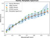 |
Fig. 1 Template spectrum of the L-type family (in black). The reflectances have been computed by averaging the Gaia spectra of (460) Scania, in blue, (2085) Henan, in orange, and (2354) Lavrov, in green. The area in light blue represents the region where the spectra of the family members identified in our analysis fall within one standard deviation. |
2 Identification of the L-type family
2.1 Identification of the family members
We followed the same procedure as was developed in Balossi et al. (2024), who demonstrated that asteroid families can be identified using only Gaia spectral data, successfully recovering Tirela/Klumpea and Watsonia, two well-characterized L-type families. We started by considering all asteroids located between semimajor axes amin = 2.50 AU and amax = 2.85 AU, eccentricities emin = 0.02 and emax = 0.1, and inclinations sin(imin) = 0.02 and sin(imax) = 0.1. The proper elements a, e and i and the absolute magnitudes H were retrieved from the Asteroid Family Portal (AFP, Novaković et al. 2022), while the albedos, ρV, and the diameters, D, were taken, when available, from the WISE/NEOWISE database (Masiero et al. 2011). A total of 1575 objects have been observed by Gaia within this region, 1116 of which had at least one albedo measurement reported in WISE/NEOWISE.
Three large confirmed L types have reflectance spectra in Gaia DR3 within this region, namely (460) Scania, (2085) Henan, and (2354) Lavrov (these last two objects also have visible-NIR spectra in Devogèle et al. 2018, the first has a visible-NIR spectrum in DeMeo et al. 2009). The Gaia spectra of these three objects, which have a larger signal-to-noise with respect to the other candidate family members in the surroundings, were averaged to create a template spectrum to represent a possible L-type family. The template spectrum is shown in black in Figure 1, where the errors represent the squared sum of the uncertainties of the spectra of all objects observed by Gaia within this region.
The objects were then classified into eight spectral classes according to the color taxonomy described in Balossi et al. (2024).
A total of 55 objects were classified as L types and were later analyzed by a χ2 similarity method, whose aim is to quantify the difference between the spectrum of a specific object and the template family spectrum. The goal is to reject possible L-types that have been wrongly assigned to the class by the classifier. We used the same definition of the χ2 as reported in Balossi et al. (2024), with the same limit at χ2 = 2. Four L types with χ2 > 2 were thus removed from the family. These are faint objects with low SNR, showing large irregular fluctuations in their spectra upon closer inspection.
The distribution in the phase space of the proper elements of the remaining 51 L types is reported in Figure 2. The L types are very spread in a, e, and sin(i) without any particular clustering. However, the distribution in the (a, H) plane, especially for a > 2.6 AU, resembles a V shape with (460) Scania at its vertex. This seems to suggest that the 51 objects might be a family that resulted from the breakup of a large L type in this region. Given the spread in the proper elements, this family must be very old. It is essential to note that some of these 51 objects may not be real family members but rather misclassified bodies or L-type interlopers. For instance, the three objects located below 2.60 AU in Figure 2 are likely interlopers, as their positions deviate significantly from the main distribution of the family. This is particularly evident when examining their locations in the (a, sin(i)) and (a, H) panels. In this regard, we repeated the whole analysis using the catalog of proper elements computed by Nesvorný et al. (2024). The membership based on this dataset is almost the same as the one determined from AFP, but it excludes from the family three small objects, two of which are among the ones below 2.60 AU. The memberships obtained from the two proper element datasets are reported in Table A.1.
We also remark here that in previous classifications, (2085) Henan was supposed to be the largest member of the family, while here it seems that (460) Scania, not included in previous clustering results obtained by the HCM, must be considered.
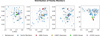 |
Fig. 2 Distribution in the phase space of the proper elements of the L types (blue circles) and all the other objects observed by Gaia (gray circles). The four largest L types are marked by diamonds. The panels are, from left to right, (a, e), (a, sin(i)), (e, sin(i)) and (a, H). |
2.2 V-shape detection and age determination
To obtain a first estimate of the family age, we fitted the slopes of the V shape in the (a, 1/D) plane following the procedure described in Spoto et al. (2015). Due to the limited number of objects in the family, we adopted the simplified procedure described in Balossi et al. (2024) for the Watsonia family and overplotted tentative V-shape boundaries corresponding to specific ages.
The diameters were taken from WISE/NEOWISE when available, otherwise, they were computed from ![Mathematical equation: $\[D=1329 \cdot 10^{-H / 5 \sqrt{\rho_{V}}}\]$](/articles/aa/full_html/2025/10/aa55527-25/aa55527-25-eq1.png) , where H is the absolute magnitude of the object and ρV the mean albedo of the family (ρV = 0.20 ± 0.07). The distribution of the family members in the (a, 1/D) plane is reported in Figure 3.
, where H is the absolute magnitude of the object and ρV the mean albedo of the family (ρV = 0.20 ± 0.07). The distribution of the family members in the (a, 1/D) plane is reported in Figure 3.
To determine the slopes of the V shape corresponding to a specific age, the Yarkovsky calibration for the family must be determined, which corresponds to the value of the drift in semimajor axis, da/dt, for a family member with unit diameter. When both da/dt and the age are known, the slope of the V shape is obtained from S = 1/(age · da/dt). Unfortunately, there are no objects in this family or L types in general with a known Yarkovsky measurement, and therefore as in Balossi et al. (2024), we decided to use the S-type (99942) Apophis as reference asteroid, whose Yarkovsky drift has been accurately computed by Fenucci et al. (2024). We thus converted the Yarkovsky drift computed for (99942) Apophis for the L-type family using the scaling formula:
![Mathematical equation: $\[\frac{d a}{d t}=\left(\frac{d a}{d t}\right)_A \frac{\sqrt{a}_A\left(1-e_A^2\right)}{\sqrt{a}\left(1-e^2\right)} \frac{D_A}{D} \frac{\rho_A}{\rho} \frac{\cos (\phi)}{\cos (\phi_A)} \frac{1-A}{1-A_A}.\]$](/articles/aa/full_html/2025/10/aa55527-25/aa55527-25-eq2.png) (1)
(1)
Here a, e, ρ, and A are, respectively, the semimajor axis, the eccentricity, the density, and the Bond albedo representative for the family. When a subscript A is present, the quantities are referred to (99942) Apophis (and taken from Moskovitz et al. 2022; Brozović et al. 2018, and Berthier et al. 2023).
The diameter D = 1 km is the diameter of a fictitious unit asteroid, while cos(ϕ) is the spin axis obliquity equal to ±1 depending on which side of the V shape is considered. For the density of (99942) Apophis, we used ρA = 2.25 g/cm3 (Farnocchia et al. 2024). The L-type density ρ is instead unknown, and we considered the reference value taken from Carry (2012), which, however, is quite inaccurate due to the limited number of large L types with accurate measurements of both mass and diameter. We thus used the reference density corresponding to C types, ρ = 1.41 ± 0.69 g/cm3, as suggested by the link between Barbarian asteroids and CO and CV meteorites, in turn related to C types, as reported in Sunshine et al. (2008) and Mahlke et al. (2023).
Assuming a relative uncertainty of 0.3, we obtained a Yarkovsky calibration for the L-type family of da/dt = (5.27 ± 1.58) · 10−4 AU/Myr.
The V shapes corresponding to ages of 1.0 Gyr and 1.5 Gyr are reported in Figure 3. Given the uncertainties on the Yarkovsky calibration and on the diameters of the family members, it is difficult to determine the exact age of the family. However, it is evident that it is quite old, around 1.0 Gyr, which is in good agreement with the spread of the proper elements. In addition, the inner side is less inclined than the outer one, thus suggesting that the latter one might be younger. This might be explained by an anisotropy in the ejection velocity field following the breakup event, which is better analyzed in Section 3. Objects on the right edge of the family may also be influenced by the strong 5:2 mean-motion resonance with Jupiter, located at 2.82 AU.
To confirm the detection of the V shape with an independent method, we applied the automated approach developed by Bolin et al. (2017). This method searches for family V shapes of unknown age and center (ac) in a population of asteroids as a function of ac and the slope K of the sides of the V. Slightly different implementations of the method exist (Bolin et al. 2017; Delbo’ et al. 2017; Ferrone et al. 2023; Walsh et al. 2013). Here, we used the so-called aw variant (Delbo’ et al. 2017; Ferrone et al. 2023): in the (a, 1/D) space a nominal-V of equation 1/D = K|a − ac| (where ∥ indicates the absolute value) is drawn. Next, we considered an “interior lobe” between the line y = K(|a − ac| + aw) and the nominal line, and an “exterior lobe” between y = K(|a − ac| − aw) and the nominal line. We counted the number of bodies within the interior Ni and exterior lobes Ne as a function of ac and K. We used the quantity ![Mathematical equation: $\[N_{i}^{2} / N_{e}\]$](/articles/aa/full_html/2025/10/aa55527-25/aa55527-25-eq3.png) as a score for the detection of the V shape. A grid of test values was created that spans a range of both ac and K. A score was calculated at each coordinate. Local maxima of this score map were candidate detections of family V shapes (Figure 4).
as a score for the detection of the V shape. A grid of test values was created that spans a range of both ac and K. A score was calculated at each coordinate. Local maxima of this score map were candidate detections of family V shapes (Figure 4).
We applied the V shape search with aw = 0.03 AU to the population of L types with 2.5 < ac < 2.8 AU and 0.2 < K < 3 AU−1 km−1. The uncertainties on ac and K were estimated by a Monte Carlo approach. We performed 104 iterations, where at each one we carried out a new V-shape search randomly varying the value of aw uniformly between 0.02 and 0.05 AU. Smaller values of aw produce visibly noisy ![Mathematical equation: $\[N_{i}^{2} / N_{e}\]$](/articles/aa/full_html/2025/10/aa55527-25/aa55527-25-eq6.png) score maps, while larger values of aw create inner and outer V-shape lobes that are too big compared to the area of the (a, 1/D) plane to scan. At each iteration, we also varied the value of the asteroid diameters and proper semimajor axis. To do so, we added to the nominal value of the proper semimajor axis a random value normally distributed with a zero mean and a standard deviation equal to the semimajor axis uncertainty. Likewise, we added to the nominal value of the diameter a random value normally distributed with a zero mean and a standard deviation equal to the diameter uncertainty. We find that the distributions of ac and K values have mean values of 2.71 AU and 2.15 AU−1 km−1, respectively, as well as standard deviations of 0.02 AU and 0.35 AU−1 km−1, respectively. We interpret these results as the detection of a V shape associated with an L-type family in the central main belt.
score maps, while larger values of aw create inner and outer V-shape lobes that are too big compared to the area of the (a, 1/D) plane to scan. At each iteration, we also varied the value of the asteroid diameters and proper semimajor axis. To do so, we added to the nominal value of the proper semimajor axis a random value normally distributed with a zero mean and a standard deviation equal to the semimajor axis uncertainty. Likewise, we added to the nominal value of the diameter a random value normally distributed with a zero mean and a standard deviation equal to the diameter uncertainty. We find that the distributions of ac and K values have mean values of 2.71 AU and 2.15 AU−1 km−1, respectively, as well as standard deviations of 0.02 AU and 0.35 AU−1 km−1, respectively. We interpret these results as the detection of a V shape associated with an L-type family in the central main belt.
We used the distribution of ac and K values to estimate the age of the family from (Eq. (2) of Ferrone et al. 2023) also during the Monte Carlo simulation. Assuming family members’ bulk densities of 1.41 ± 0.69 g/cm3, we obtained a family age of 1.1 ± 0.6 Gyr.
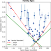 |
Fig. 3 Family members (in blue) in the (a, 1/D) plane fitted by V shapes corresponding to different ages. The green continuous line corresponds to 1.5 Gyr and the red dashed line to 1.0 Gyr. |
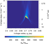 |
Fig. 4 Result of the V-shape-searching method. The value of |
![Mathematical equation: $\[N_{in}^2 / N_{out}\]$](/articles/aa/full_html/2025/10/aa55527-25/aa55527-25-eq4.png)
![Mathematical equation: $\[C=1 / K \sqrt{p_{V}} / 1329\]$](/articles/aa/full_html/2025/10/aa55527-25/aa55527-25-eq5.png)
3 Numerical simulation of the family
We consider here a numerical simulation of the evolution of the family, with the goal of confirming its dispersion in the space of the osculating elements and its age. To integrate the system, we used the N-body integrator REBOUND (Rein & Liu 2012) and the REBOUNDx package to incorporate the Yarkovsky effect (Tamayo et al. 2020; Ferich et al. 2022).
The semimajor axis aPB, eccentricity ePB, and inclination iPB of the parent body at the moment of breakup were taken as averages of the proper elements of the family members retrieved from Gaia. The true anomaly fPB, the longitude of the perihelion ωPB and the longitude of the ascending node ΩPB were assumed to be 10, 180, and 130 degrees, respectively, because by successive attempts, we verified that these were the best values reproducing the observed clusters in the proper elements phase space. Very different values produced similar results, but a shift of the final state in i and/or e.
281 fragments with the same diameter D of the family members observed by Gaia were placed at the breakup position. In our simulation, we prioritized fragments with smaller diameters, including only five larger fragments to account for the presence of bigger objects. The fragments were assigned an isotropic ejection velocity field, where the value of the breakup velocity vej was determined from Carruba et al. (2003), where we assumed the density of the parent body ρPB = 1.41 gm/c3, same as the family members, and the fraction of specific energy going into the fragmentation kinetic energy fKE = 0.01, to maintain the family as compact as possible. The radius of the parent body RPB was initially determined as the sum of the size of the largest and third largest family members (Tanga et al. 1999), which resulted in Rpb = 18 km. However, generating a synthetic size distribution using the geometric model described in Tanga et al. (1999) we found that the size distribution of the 51 family members observed by Gaia was better described by a parent body with radius Rpb = 30 km (Figure 10), which resulted in a mass ratio between the largest fragment and the parent body of 0.04. This is a small value, but still compatible with other families observed in the main belt, such as Koronis and Maria (Tanga et al. 1999). In our simulations, we therefore assumed RPB = 30 km.
The fragments were then assigned an isotropic ejection velocity field with the ejection velocity randomly oriented in space. The module of the ejection velocity was modeled from v = vej(DPB/D)αEV (Bolin et al. 2018), where αEV was assumed to be equal to one. The Yarkovsky effect was also added to the simulation (Ferich et al. 2022). The REBOUNDx Yarkovsky model requires as input parameters the diameters, the albedos, which were taken from NEOWISE, and the densities, assumed to be ρ = 1.41 ± 0.69 g/cm3 (see Section 2).
The system was integrated in time until 630 million years under the gravitational forces of the giant planets and the Yarkovsky effect using WHFast, a symplectic Wisdom-Holman integrator (Rein & Tamayo 2015; Wisdom & Holman 1991), with a timestep of 30 days. Snapshots of the simulation were taken every 10 million years. The final state of the system is reported in Figure 5, where the mean proper elements of the synthetic fragments are compared to the Gaia family members. Proper elements were computed following the methodology of Knežević & Milani (2003), which involves (i) numerical integration of asteroid orbits within a realistic dynamical model for 2 Myr in the past and 10 Myr in the future; (ii) digital filtering to remove short-period perturbations; and (iii) Fourier analysis of the filtered output to eliminate the main forced terms. Starting from the initial conditions provided by the propagated simulated orbital elements over 630 Myr, we then derived the proper elements corresponding to each set of simulated orbital elements.
The distribution of the synthetic family members reproduces the observed one. The only objects that are not reproduced are the three below 2.60 AU, which, as already discussed in Section 2.1, are likely interlopers. The small residual differences can be explained by the possibility that the observed family is slightly older than the synthetic one (~ 1 Gyr vs 0.63 Gyr). In addition, it was observed that the orbital elements of the breakup position affect the positions of the synthetic clusters in the proper element phase space. The synthetic distribution is also influenced by the details of the ejection velocity field, which is far more complex than the simplified model we used.
Overall, the sides of the synthetic V shape are in good agreement with the observed one. As mentioned in Section 2.2, the V shape is not symmetric, but the slope of the outer side is larger than the inner one. Determining the age of the family from the Yarkovsky calibration results in an age of about 500 Myr for the outer side and an age of 1000 Myr for the inner side. This quite large variation can be explained by assuming that the initial velocity field was not isotropic and that the fragments on the inner side have been ejected faster than the fragments on the outer side. The difference in the ejection velocity needed to explain the observed difference can be computed from Bolin et al. (2018) as ![Mathematical equation: $\[\Delta v_{E J}=\frac{n}{2}|a_{1}-a_{2}|(\frac{D}{D_{P B}})^{\alpha_{E V}}\]$](/articles/aa/full_html/2025/10/aa55527-25/aa55527-25-eq7.png) , where n is the mean motion of the parent body, |a1 − a2| is the difference in semimajor axis of two hypothetical objects of diameters D located on the sides of the V shape, DPB is the diameter of the parent body and αEV = 1.
, where n is the mean motion of the parent body, |a1 − a2| is the difference in semimajor axis of two hypothetical objects of diameters D located on the sides of the V shape, DPB is the diameter of the parent body and αEV = 1.
It is found that a difference of around 36 m/s in the initial ejection velocity field can explain the observed difference in slope.
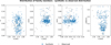 |
Fig. 5 Comparison between the proper elements of the family members observed by Gaia (gray circles) and the mean proper elements of the synthetic family members integrated in REBOUND (blue stars). The panels are, respectively, from left to right, (a, e), (a, sin(i)), (e, sin(i)), and (a, 1/D). |
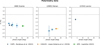 |
Fig. 6 Polarimetric measurements reported in the literature for the objects belonging to the L-type family. The asteroids with data are, from left to right, (460) Scania, (2085) Henan, and (2354) Lavrov. |
4 Additional data – polarimetry and spin obliquity
We searched the literature for additional data that could tell more about the family without being limited to the taxonomy and Gaia spectra.
Barbarian asteroids can be recognized from polarimetric measurements as they show a negative polarization at large phase angles, while normal asteroids at the same phase angles present a transition to a positive polarization (Cellino et al. 2006; Cellino et al. 2014; Gil-Hutton et al. 2008; Gil-Hutton et al. 2014).
Barbarian asteroids have been the subject of extensive spectroscopic studies in the literature, for example by Devogèle et al. (2018), who found that all observed Barbarians belong to the L-type spectral class. The visible and near-infrared spectra of these objects are interpreted as being consistent with a notably high abundance of spinel on their surfaces.
We searched several polarimetric databases published in the literature: the Torino catalog (Cellino et al. 2005), the Belskaya Asteroid Polarimetry (Belskaya et al. 2010), the CASLEO survey (López-Sisterna et al. 2019), the Asteroid Polarimetric Database (APD, Lupishko 2022), and finally the Calern Asteroid Polarisation Survey (CAPS, Bendjoya et al. 2022).
Only three family members have been observed: (460) Scania, (2085) Henan, and (2354) Lavrov, whose measurements are reported in Figure 6. There is just a single data point for (2354) Lavrov at a small phase angle, which is not enough to draw any conclusions about its nature. (2085) Henan has very negative polarization at large phase angles and therefore is a good Barbarian candidate, a result which was already reported in the literature, for example by Devogèle et al. (2018). However, these observations may also be consistent with the phase-polarization behavior of certain peculiar Ch-type asteroids, as illustrated in Figure 8 in Bendjoya et al. (2022). Finally, the six measurements for (460) Scania present a large negative polarization, and they cover a wide range in phase angles, strongly supporting its classification as a Barbarian.
We also searched the literature for the spin obliquities of the family members. The V shape is the result of the drift in semimajor axis of an object due to the Yarkovsky effect, which depends on the orientation of its rotation axis. Prograde rotators with a spin obliquity smaller than 90 degrees drift outward, while retrograde rotators with a spin obliquity larger than 90 degrees drift inward. Therefore, there should be a correlation between the position of an object on the V shape and its spin obliquity (Vokrouhlický et al. 2015; Athanasopoulos et al. 2022; Athanasopoulos et al. 2024).
The spin obliquities were taken from three sources: the LCDB database2 (Warner et al. 2021), and the works by Ďurech & Hanuš (2023) and Cellino et al. (2024), who both determined the spin states using Gaia DR3 photometry. For objects without measurements in any of these works, we searched the rocks database (Berthier et al. 2023) for additional data.
We combined the data from the three studies to retrieve the spin obliquities of the L-types. For objects observed by more than one study, we adopted the following decision scheme: first, we prioritized measurements from LCDB with a good quality flag. Next, we considered the data from Ďurech & Hanuš (2023). We then included measurements from LCDB associated with a poor quality flag, and finally, we included data from Cellino et al. (2024).
The results are shown in Figure 7, from which it can be seen that there is a very good correlation between the obliquity and the position on the V shape. There are only four objects that do not respect this correlation, two of which are very small and located far in semimajor axis from the rest of the family (one of these is one of the three objects below 2.60 AU already discussed in Section 2.1). The blue point around (2.65 AU, 0.20 km−1) might be an interloper, or its obliquity measurement might be flawed. Finally, there is a retrograde rotator around 2.72 AU, where prograde rotation is expected. However, this object lies very close to the center of the family, and its spin state may have been recently altered by collisions or other nongravitational effects, such as the YORP effect.
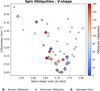 |
Fig. 7 V shape of the family in the (a, 1/D) plane with the objects marked according to the value of their spin obliquity. Gray circles are objects for which the spin is unknown. Gray stars have a known spin period, but no determination of their spin axis obliquity. Finally, diamonds have a known spin axis obliquity, which is indicated by their color: red are retrograde rotators, and blue are prograde. |
5 Comparison to literature
5.1 Comparison to HCM algorithms
We searched the literature to check if the L-type family had already been identified by any of the most commonly used family classification schemes, all based on HCM algorithms. In particular, we compared with Ast-DyS3 (Milani et al. 2014), AFP4 (Novaković et al. 2022) and finally with the work of Nesvorny (2024)5. Each of these classification systems reports different families in the region.
None of the objects we classify as family members is assigned to any family by AFP, except for a few objects included in the Agnia family. These objects, however, are clear interlopers, both in spectroscopic terms, since Agnia is an S-type family, and in the phase space of the proper elements, as these objects are well separated from the core of the Agnia family.
Ast-DyS reports four families overlapping with our family, namely 29841, 11882, 12739, and 17392, which, however, are very small and faint clusters and have no objects in common with the L-type family.
Nesvorny (2024) is the only scheme identifying an L-type family in this region, having (2085) Henan as the largest member. However, even this system fails to link to the family the larger L types and misses the V shape described in Section 2.
Instead of relying on literature classification schemes, we ran an independent HCM algorithm to identify families in this region. Even when changing the value of the limit cutoff velocity used to define families, the L-type family is never identified by the HCM.
This is not surprising since the family is very old and spread in the proper elements phase space, making it almost impossible for the HCM to identify it.
Finally, Mothé-Diniz et al. (2005) analyzed the taxonomy of asteroid families identified by their version of the HCM and they report a cluster of 37 objects with (2354) Lavrov as the largest member. Unfortunately, they do not report anywhere the full membership of the clump. However, five of these objects had available spectra at the time, plus another object linked to the clump at larger cutoff velocities. These objects are (2354) Lavrov itself, (3349) Manas, (3844) Lujiaxi, (4426) Roerich, (4726) Federer, and (5840) Raybrown, which were all classified as L types. Three of these objects, 2354, 3844, and 5840 have also been classified as L types by the Gaia color taxonomy and therefore included in our family. The other three objects were classified differently from the L class, even if their spectra closely resemble the family template. This evidence suggests that the color taxonomy might lose some L types to other classes due to the intrinsic limitations of Gaia spectra and the taxonomy itself. A search in literature is thus necessary to verify how objects in this region were classified by previous works, and to understand if the family could have been identified even without Gaia spectra.
5.2 Comparison to literature taxonomy
To prove that the L-type family is not the result of a bad classification of Gaia spectra, we ran an independent analysis using taxonomic classifications reported in the literature. We considered the sample observed by Gaia in this region and searched the literature for previous taxonomy classifications of these objects. For this purpose, we used the Python package rocks (Berthier et al. 2023), which for each object lists all the spectral classes in which the object has been classified, along with the literature reference, the taxonomy scheme, the method of observation (photometry or spectroscopy), and the wave range of the observation (VIS, NIR, or VISNIR).
For objects with multiple classifications, we considered it an L type if more than half of the classifications corresponded to the L-class (or similar classes, such as the Ld-class of Bus & Binzel 2002), giving priorities to classifications obtained from spectroscopic observations.
We found 81 objects that have been classified as L types in the literature. These objects are shown in the (a, 1/D) plane in Figure 8, where a V shape is clearly recognizable. Three objects might be interlopers since they are lying outside the V shape: the two points around (2.54 AU, 0.23 km−1) and the point at (2.61 AU, 0.14 km−1). An analysis of the spin obliquity showed that this last point is a prograde rotator, which is in contrast with its position on the V shape. For the other objects, there was instead a very good correspondence of the spin obliquity with the position on the V shape, especially for the outer side. On the inner side, three small objects with diameters between 3 and 4 km turned out to be prograde rotators, thus they might be interlopers, or the measurements of their spin obliquity might be wrong.
Figure 8 also reports the position of the L types identified using Gaia spectra. There is a general good agreement between the L types obtained from the literature and Gaia, especially at large diameters. The large object close to the vertex of the V shape that is classified as L by Gaia and not by the literature is (1007) Pawlowia. This object has been classified five times in the literature, twice as S (Mahlke et al. 2022; DeMeo & Carry 2013), twice as L (Sergeyev & Carry 2021; Carvano et al. 2010), and once as K (Bus & Binzel 2002). However, its albedo of 0.13 is unusually low for an S-type, thus suggesting that it is more likely associated with the M or L types. (1007) Pawlowia has not been included in the family because of the criteria we adopted, even if there is a good probability that it is an L type. Additional spectroscopic observations of this object are needed to characterize its true nature. If it is indeed an L-type, the family would become particularly intriguing, as it would then feature two largest remnants with nearly identical sizes.
At smaller diameters, the two V shapes are still compatible, especially since they share the same vertex and similar slopes, although there is less agreement between the two classifications. In addition, the L types identified from the literature seem to complete the Gaia V shape, especially at small diameters in the inner side.
Due to the limitations of the color taxonomy and the low SNR of the Gaia spectra of small objects, it was predicted that some small objects listed as L types in the literature would have been lost in the Gaia classification.
Less expected instead was to find objects classified as L types from Gaia spectra but not in the literature. We therefore analyzed the literature taxonomy of these 33 objects and the results are shown in Figure 9. Two objects were classified as S types from spectroscopic observations. One of them is (1007) Pawlowia, which was already discussed, while the other one is (4619) Polyakhova. This object was classified twice in the literature, both based on spectroscopic observations, as S type by Mahlke et al. (2022) and as L type by Bus & Binzel (2002). (4619) Polyakhova might therefore be an L type, but additional observations are needed to confirm its nature.
The classification of 19 objects was instead based on photometric observations, which are less precise than spectroscopy. Therefore, it would not be surprising if some of these objects, especially the ones classified as S or D types, would turn out to be L types. The objects classified as C, B, or X types might be the result of a wrong classification of Gaia spectra or poor quality photometric measurements.
Finally, 12 objects never received a taxonomic classification before this work.
In the following, Gaia membership refers to the family membership derived from L types identified using Gaia spectra, literature membership corresponds to the membership based on L types reported in the literature, excluding the three interlopers discussed in Figure 8, and combined membership includes all L types identified by either classification.
Figure 10 reports the size distributions of the three memberships. The Gaia membership presents an unusual size distribution due to the presence of two largest remnants (Scania and Pawlowia) of similar size. The size distribution determined from the literature is instead consistent with other known families since it does not include (1007) Pawlowia. Figure 10 also reports the size distribution obtained from the geometric model developed by Tanga et al. (1999) for a parent body of radius Rpb = 30 km and a mass ratio between the largest fragment and the parent body mratio = 0.04 (see Section 3). The slope of the simulated size distribution is similar to those of both Gaia and literature memberships at large diameters, while, as expected, it includes more objects at smaller diameters. Unfortunately, the geometric model does not help to clarify whether (1007) Pawlowia is an interloper or an actual family member.
Overall, the agreement between the Gaia and literature memberships and the similarities between the two V shapes show that the L-type family identified in this work is real. More observations are needed to establish the exact membership of the family at small diameters and to determine the nature of some interesting objects, (1007) Pawlowia in particular.
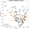 |
Fig. 8 V shape in the (a, 1/D) plane of the L types identified from the literature (orange diamonds) and from Gaia spectra (blue circles). |
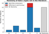 |
Fig. 9 Literature taxonomy for the objects classified as L from Gaia spectra but not in the literature. In red, the objects for which the literature taxonomy has been determined from spectroscopy, in blue from photometry, and in gray objects that were never classified before this work. |
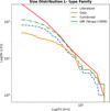 |
Fig. 10 Size distributions for the Gaia membership (orange, solid line), literature membership (blue, dashed line), combined membership (green, dash-dotted line), and the geometric model by Tanga et al. (1999) (red, solid line). |
6 Conclusions
In this paper, we have presented the identification of the family of Scania, an L-type family in the middle main belt, based initially on the analysis of a taxonomy derived from Gaia DR3 spectra. Although our method solves some of the limitations of the HCM, it is not excluded that it still presents some biases, particularly since it assumes that the family is compositionally homogeneous.
The color taxonomy that we adopt is known to have some limitations, in particular due to its tendency to classify into the most common spectral type (the S and C classes) objects that would belong to other less common spectral types. In addition, the color taxonomy might fail in classifying faint objects characterized by a low SNR and flawed spectra.
Because of these reasons, the family membership obtained from this work cannot be considered definitive. Table A.1 in the Appendix provides a list of the L types identified from Gaia spectra and from previous literature observations, along with their proper elements, albedos, and diameters.
The comparison between the Gaia and literature memberships is in good agreement, especially at large diameters. Both memberships produce a well-defined V shape in the (a, 1/D) plane, sharing the same vertex and similar slopes. The real family membership could thus be close to the combination of the Gaia and literature memberships. We hope that with the next Gaia data release, expected for 2026, it will be possible to clarify the actual membership of this family.
A more careful analysis is also necessary to identify any interlopers within the family. In particular, in the Gaia membership the two largest fragments present a similar size, resulting in a peculiar size distribution. The largest fragment, (460) Scania, was proven to be an L type by previous spectroscopic observations and by polarimetry measurements. (1007) Pawlowia instead does not have any polarimetry measurement, and its spectra and albedo are contradictory. Additional observations of this object are necessary to determine its true nature and to assess whether the family indeed contains two largest remnants of similar size.
An analysis of the V shape of the family confirms that it is quite old, around 1 Gyr, and its members are very spread in the proper elements phase space. This explains why the HCM always failed to identify this family. In the best cases, small subgroups were linked together (Mothé-Diniz et al. 2005; Milani et al. 2014).
This study confirms the interest of combining dynamical and physical properties to identify and characterize asteroid families, especially in difficult cases. Such mixed approaches are certainly going to develop to a much larger extent, with the growing set of data collected by large forthcoming surveys on fainter and fainter objects.
An open question remains the significance of the identified families composed of the rather uncommon L-type asteroids, with respect to the supposedly ancient formation age of their parent body, in an environment rich in poorly altered chondritic material and CAIs. We can speculate that, if they belong to a first generation of asteroids, only fragments of larger objects survive today, associated with dispersed and old families such as Henan and Scania. Additional high-quality spectra on smaller asteroids in the belt are needed to disentangle L types from similar spectra and better understand this scenario.
Acknowledgements
This work presents results from the European Space Agency (ESA) space mission Gaia. Gaia data are being processed by the Gaia Data Processing and Analysis Consortium (DPAC). Funding for the DPAC is provided by national institutions, in particular, the institutions participating in the Gaia Multilateral Agreement (MLA). The Gaia mission website is https://www.cosmos.esa.int/Gaia. The Gaia archive website is https://archives.esac.esa.int/Gaia. RB Doctoral contract is funded by Universitè de la Côte d’Azur. This project was financed in part by the French Programme National de Planetologie, and by the BQR program of Observatoire de la Côte d’Azur. We made use of the software products: SsODNet VO service of IMCCE, Observatoire de Paris, and the associated rocks library6 (Berthier et al. 2023); Astropy, a community-developed core Python package for Astronomy (Astropy Collaboration 2013, 2018, 2022); Matplotlib (Hunter 2007). This work was supported by the French government through the France 2030 investment plan managed by the National Research Agency (ANR), as part of the Initiative of Excellence Université Côte d’Azur under reference number ANR-15-IDEX-01. The authors are grateful to the Université Côte d’Azur’s Center for High-Performance Computing (OPAL infrastructure) for providing resources and support.
Appendix
Membership for the L-type family retrieved in this work.
References
- Astropy Collaboration (Robitaille, T. P., et al.) 2013, A&A, 558, A33 [NASA ADS] [CrossRef] [EDP Sciences] [Google Scholar]
- Astropy Collaboration (Price-Whelan, A. M., et al.) 2018, AJ, 156, 123 [Google Scholar]
- Astropy Collaboration (Price-Whelan, A. M., et al.) 2022, ApJ, 935, 167 [NASA ADS] [CrossRef] [Google Scholar]
- Athanasopoulos, D., Hanuš, J., Avdellidou, C., et al. 2022, A&A, 666, A116 [NASA ADS] [CrossRef] [EDP Sciences] [Google Scholar]
- Athanasopoulos, D., Hanuš, J., Avdellidou, C., et al. 2024, A&A, 690, A215 [NASA ADS] [CrossRef] [EDP Sciences] [Google Scholar]
- Balossi, R., Tanga, P., Sergeyev, A., Cellino, A., & Spoto, F. 2024, A&A, 688, A221 [NASA ADS] [CrossRef] [EDP Sciences] [Google Scholar]
- Belskaya, I. N., Levasseur-Regourd, A. C., Cellino, A., et al. 2010, Belskaya Asteroid Polarimetry V1.0, NASA Planetary Data System, id. EAR-A-I0942/I0943-3-BELSKAYAPOL-V1.0 [Google Scholar]
- Bendjoya, P., Cellino, A., Rivet, J. P., et al. 2022, A&A, 665, A66 [NASA ADS] [CrossRef] [EDP Sciences] [Google Scholar]
- Berthier, J., Carry, B., Mahlke, M., & Normand, J. 2023, A&A, 671, A151 [NASA ADS] [CrossRef] [EDP Sciences] [Google Scholar]
- Bolin, B. T., Delbo, M., Morbidelli, A., & Walsh, K. J. 2017, Icarus, 282, 290 [CrossRef] [Google Scholar]
- Bolin, B. T., Walsh, K. J., Morbidelli, A., & Delbó, M. 2018, MNRAS, 473, 3949 [Google Scholar]
- Bottke, Jr., W. F., Vokrouhlický, D., Rubincam, D. P., & Nesvorný, D. 2006, Annu. Rev. Earth Planet. Sci., 34, 157 [CrossRef] [Google Scholar]
- Brož, M., Morbidelli, A., Bottke, W. F., et al. 2013, A&A, 551, A117 [Google Scholar]
- Brozović, M., Benner, L. A. M., McMichael, J. G., et al. 2018, Icarus, 300, 115 [CrossRef] [Google Scholar]
- Bus, S. J., & Binzel, R. P. 2002, Icarus, 158, 146 [Google Scholar]
- Carruba, V., Burns, J. A., Bottke, W., & Nesvorný, D. 2003, Icarus, 162, 308 [NASA ADS] [CrossRef] [Google Scholar]
- Carry, B. 2012, Planet. Space Sci., 73, 98 [CrossRef] [Google Scholar]
- Carvano, J. M., Hasselmann, P. H., Lazzaro, D., & Mothé-Diniz, T. 2010, A&A, 510, A43 [NASA ADS] [CrossRef] [EDP Sciences] [Google Scholar]
- Cellino, A., Hutton, R. G., Di Martino, M., et al. 2005, Icarus, 179, 304 [CrossRef] [Google Scholar]
- Cellino, A., Belskaya, I., Bendjoya, P., et al. 2006, Icarus, 180, 565 [NASA ADS] [CrossRef] [Google Scholar]
- Cellino, A., Bagnulo, S., Tanga, P., Novakovic, B., & Delbo, M. 2014, MNRAS, 439, L75 [NASA ADS] [CrossRef] [Google Scholar]
- Cellino, A., Tanga, P., Muinonen, K., & Mignard, F. 2024, A&A, 687, A277 [NASA ADS] [CrossRef] [EDP Sciences] [Google Scholar]
- Delbo’, M., Walsh, K., Bolin, B., Avdellidou, C., & Morbidelli, A. 2017, Science, 357, 1026 [NASA ADS] [CrossRef] [Google Scholar]
- Delbo, M., Avdellidou, C., & Morbidelli, A. 2019, A&A, 624, A69 [NASA ADS] [CrossRef] [EDP Sciences] [Google Scholar]
- DeMeo, F. E., & Carry, B. 2013, Icarus, 226, 723 [NASA ADS] [CrossRef] [Google Scholar]
- DeMeo, F. E., Binzel, R. P., Slivan, S. M., & Bus, S. J. 2009, Icarus, 202, 160 [Google Scholar]
- Devogèle, M., Tanga, P., Cellino, A., et al. 2018, Icarus, 304, 31 [Google Scholar]
- Ďurech, J., & Hanuš, J. 2023, A&A, 675, A24 [NASA ADS] [CrossRef] [EDP Sciences] [Google Scholar]
- Farnocchia, D., Vokrouhlicky, D., Capek, D., Chesley, S. R., & DellaGiustina, D. N. 2024, in LPI Contributions, 3006, Apophis T-5 Workshop, 2046 [Google Scholar]
- Fenucci, M., Micheli, M., Gianotto, F., et al. 2024, A&A, 682, A29 [NASA ADS] [CrossRef] [EDP Sciences] [Google Scholar]
- Ferich, N., Baronett, S. A., Tamayo, D., & Steffen, J. H. 2022, ApJS, 262, 41 [Google Scholar]
- Ferrone, S., Delbo, M., Avdellidou, C., et al. 2023, A&A, 676, A5 [NASA ADS] [CrossRef] [EDP Sciences] [Google Scholar]
- Gaia Collaboration (Galluccio, L., et al.) 2023, A&A, 674, A35 [NASA ADS] [CrossRef] [EDP Sciences] [Google Scholar]
- Gil-Hutton, R., Mesa, V., Cellino, A., et al. 2008, A&A, 482, 309 [NASA ADS] [CrossRef] [EDP Sciences] [Google Scholar]
- Gil-Hutton, R., Cellino, A., & Bendjoya, P. 2014, A&A, 569, A122 [EDP Sciences] [Google Scholar]
- Hunter, J. D. 2007, Comput. Sci. Eng., 9, 90 [NASA ADS] [CrossRef] [Google Scholar]
- Knežević, Z., & Milani, A. 2003, A&A, 403, 1165 [Google Scholar]
- López-Sisterna, C., García-Migani, E., & Gil-Hutton, R. 2019, A&A, 626, A42 [EDP Sciences] [Google Scholar]
- Lupishko, D. 2022, Asteroid Polametric Database (APD) Bundle V2.0, NASA Planetary Data System, urn:nasa:pds:asteroid_polarimetric_database::2.0 [Google Scholar]
- Mahlke, M., Carry, B., & Mattei, P. A. 2022, A&A, 665, A26 [NASA ADS] [CrossRef] [EDP Sciences] [Google Scholar]
- Mahlke, M., Eschrig, J., Carry, B., Bonal, L., & Beck, P. 2023, A&A, 676, A94 [NASA ADS] [CrossRef] [EDP Sciences] [Google Scholar]
- Masiero, J. R., Mainzer, A. K., Grav, T., et al. 2011, ApJ, 741, 68 [Google Scholar]
- Migliorini, F., Zappalà, V., Vio, R., & Cellino, A. 1995, Icarus, 118, 271 [NASA ADS] [CrossRef] [Google Scholar]
- Milani, A., Cellino, A., Knežević, Z., et al. 2014, Icarus, 239, 46 [NASA ADS] [CrossRef] [Google Scholar]
- Moskovitz, N. A., Wasserman, L., Burt, B., et al. 2022, Astron. Comput., 41, 100661 [NASA ADS] [CrossRef] [Google Scholar]
- Mothé-Diniz, T., Roig, F., & Carvano, J. M. 2005, Icarus, 174, 54 [CrossRef] [Google Scholar]
- Nesvorny, D. 2024, Nesvorny HCM Asteroid Families, NASA Planetary Data System, urn:nasa:pds:ast.nesvorny.families::2.0 [Google Scholar]
- Nesvorný, D., Roig, F., Vokrouhlický, D., & Brož, M. 2024, ApJS, 274, 25 [Google Scholar]
- Novaković, B., Vokrouhlický, D., Spoto, F., & Nesvorný, D. 2022, Celest. Mech. Dyn. Astron., 134, 34 [NASA ADS] [CrossRef] [Google Scholar]
- Parker, A., Ivezić, Ž., Jurić, M., et al. 2008, Icarus, 198, 138 [Google Scholar]
- Rein, H., & Liu, S. F. 2012, A&A, 537, A128 [NASA ADS] [CrossRef] [EDP Sciences] [Google Scholar]
- Rein, H., & Tamayo, D. 2015, MNRAS, 452, 376 [Google Scholar]
- Sergeyev, A. V., & Carry, B. 2021, A&A, 652, A59 [NASA ADS] [CrossRef] [EDP Sciences] [Google Scholar]
- Spoto, F., Milani, A., & Knežević, Z. 2015, Icarus, 257, 275 [NASA ADS] [CrossRef] [Google Scholar]
- Sunshine, J. M., Connolly, H. C., McCoy, T. J., Bus, S. J., & La Croix, L. M. 2008, Science, 320, 514 [Google Scholar]
- Tamayo, D., Rein, H., Shi, P., & Hernandez, D. M. 2020, MNRAS, 491, 2885 [NASA ADS] [CrossRef] [Google Scholar]
- Tanga, P., Cellino, A., Michel, P., et al. 1999, Icarus, 141, 65 [NASA ADS] [CrossRef] [Google Scholar]
- Vokrouhlický, D., Brož, M., Bottke, W. F., Nesvorný, D., & Morbidelli, A. 2006, Icarus, 182, 118 [Google Scholar]
- Vokrouhlický, D., Bottke, W. F., Chesley, S. R., Scheeres, D. J., & Statler, T. S. 2015, in Asteroids IV, eds. P. Michel, F. E. DeMeo, & W. F. Bottke (University of Arizona Press), 509 [Google Scholar]
- Walsh, K. J., Delbó, M., Bottke, W. F., Vokrouhlický, D., & Lauretta, D. S. 2013, Icarus, 225, 283 [NASA ADS] [CrossRef] [Google Scholar]
- Warner, B. D., Harris, A. W., & Pravec, P. 2021, Asteroid Lightcurve Database (LCDB) Bundle V4.0, NASA Planetary Data System, urn:nasa:pds:ast-lightcurve-database::4.0 [Google Scholar]
- Wisdom, J., & Holman, M. 1991, AJ, 102, 1528 [Google Scholar]
- Zappala, V., Cellino, A., Farinella, P., & Knezevic, Z. 1990, AJ, 100, 2030 [CrossRef] [Google Scholar]
All Tables
All Figures
|
Fig. 1 Template spectrum of the L-type family (in black). The reflectances have been computed by averaging the Gaia spectra of (460) Scania, in blue, (2085) Henan, in orange, and (2354) Lavrov, in green. The area in light blue represents the region where the spectra of the family members identified in our analysis fall within one standard deviation. |
| In the text | |
|
Fig. 2 Distribution in the phase space of the proper elements of the L types (blue circles) and all the other objects observed by Gaia (gray circles). The four largest L types are marked by diamonds. The panels are, from left to right, (a, e), (a, sin(i)), (e, sin(i)) and (a, H). |
| In the text | |
|
Fig. 3 Family members (in blue) in the (a, 1/D) plane fitted by V shapes corresponding to different ages. The green continuous line corresponds to 1.5 Gyr and the red dashed line to 1.0 Gyr. |
| In the text | |
|
Fig. 4 Result of the V-shape-searching method. The value of |
| In the text | |
|
Fig. 5 Comparison between the proper elements of the family members observed by Gaia (gray circles) and the mean proper elements of the synthetic family members integrated in REBOUND (blue stars). The panels are, respectively, from left to right, (a, e), (a, sin(i)), (e, sin(i)), and (a, 1/D). |
| In the text | |
|
Fig. 6 Polarimetric measurements reported in the literature for the objects belonging to the L-type family. The asteroids with data are, from left to right, (460) Scania, (2085) Henan, and (2354) Lavrov. |
| In the text | |
|
Fig. 7 V shape of the family in the (a, 1/D) plane with the objects marked according to the value of their spin obliquity. Gray circles are objects for which the spin is unknown. Gray stars have a known spin period, but no determination of their spin axis obliquity. Finally, diamonds have a known spin axis obliquity, which is indicated by their color: red are retrograde rotators, and blue are prograde. |
| In the text | |
|
Fig. 8 V shape in the (a, 1/D) plane of the L types identified from the literature (orange diamonds) and from Gaia spectra (blue circles). |
| In the text | |
|
Fig. 9 Literature taxonomy for the objects classified as L from Gaia spectra but not in the literature. In red, the objects for which the literature taxonomy has been determined from spectroscopy, in blue from photometry, and in gray objects that were never classified before this work. |
| In the text | |
|
Fig. 10 Size distributions for the Gaia membership (orange, solid line), literature membership (blue, dashed line), combined membership (green, dash-dotted line), and the geometric model by Tanga et al. (1999) (red, solid line). |
| In the text | |
Current usage metrics show cumulative count of Article Views (full-text article views including HTML views, PDF and ePub downloads, according to the available data) and Abstracts Views on Vision4Press platform.
Data correspond to usage on the plateform after 2015. The current usage metrics is available 48-96 hours after online publication and is updated daily on week days.
Initial download of the metrics may take a while.