| Issue |
A&A
Volume 702, October 2025
|
|
|---|---|---|
| Article Number | A276 | |
| Number of page(s) | 9 | |
| Section | Stellar structure and evolution | |
| DOI | https://doi.org/10.1051/0004-6361/202555830 | |
| Published online | 30 October 2025 | |
The pre-eruption state of T CrB as observed with ALMA in 2024
1
European Southern Observatory, Karl-Schwarzschild-Strasse 2, 85748 Garching, Germany
2
Departament de Física, EEBE, Universitat Politècnica de Catalunya, c/Eduard Maristany 16, 08019 Barcelona, Spain
3
Institut d’Estudis Espacials de Catalunya (IEEC), 08860 Castelldefels (Barcelona), Spain
4
Departamento de Física, Universidad de Santiago de Chile, Av. Victor Jara 3659, Santiago, Chile
5
Center for Interdisciplinary Research in Astrophysics and Space Exploration (CIRAS), USACH, Santiago, Chile
6
Max-Planck Institut für extraterrestrische Physik (MPE), Giessenbachstr. 1, 85748 Garching, Germany
⋆ Corresponding authors: This email address is being protected from spambots. You need JavaScript enabled to view it.
; This email address is being protected from spambots. You need JavaScript enabled to view it.
Received:
5
June
2025
Accepted:
4
September
2025
Abstract
Context. T CrB is a nearby symbiotic binary and a recurrent nova with a period of around 80 years. The next eruption is expected to take place in 2025 or 2026. As part of a global multi-wavelength campaign on the event, we have obtained time on the Atacama Large mm/sub-mm Array to observe the object between 42 GHz and 407 GHz.
Aims. In this first paper on our results, we present our pre-eruption observations made in ALMA frequency Bands 1, 3, 4, 6, 7, and 8 in August to November 2024 and constrain the properties of the environment into which the imminent next nova will erupt.
Methods. We calibrated and imaged our ALMA data following the standard ALMA procedures, searched for line emission, and constructed a spectrum from the points for orbital phase 0.43 (August 2024) from 44 GHz to 350 GHz. We compared this with the spectra we measured in the VLA data obtained by Linford et al. in 2016-2017 over the upper half of their frequency range (13.5 GHz to 35 GHz). We created aggregate bandwidth images from all our 2024 data and, for maximum angular resolution, from the band 7 and 8 data, from which we computed an upper limit on the brightness temperature in an annulus with radius 0.8 arcsec – 1.6 arcsec.
Results. In the second half of 2024, after the end of its latest high state, the quiescent T CrB was a faint millimeter source with a spectral energy distribution well described by a power law with index α = 0.56 ± 0.11 and a flux density of ca. 0.1 mJy at 44 GHz and 0.4 mJy at 400 GHz. There is no significant line emission. This is in agreement with expectations for free-free emission from the partially ionized wind of the red giant donor star and, in extrapolation to 35 GHz, a factor of 5 fainter than the emission observed in 2016-2017 during the latest high state. Comparing the spectra from that high state between 13.5 GHz and 35 GHz with our spectrum from 2024, our spectrum is softer. The spectral index is on average lower by 0.34 ± 0.11. Our per-band and aggregate bandwidth images of T CrB show an unresolved point source with no evidence of extended structure.
Conclusions. A simple model of a free-free emitting, fully ionized stellar wind seems to describe well the 2016-2017 high state of T CrB but not our 2024 ALMA measurements, with their low flux and high turnover frequency suggesting that in 2024 the wind was far from fully ionized.
Key words: binaries: symbiotic / novae, cataclysmic variables / stars: individual: T CrB
© The Authors 2025
 Open Access article, published by EDP Sciences, under the terms of the Creative Commons Attribution License (https://creativecommons.org/licenses/by/4.0), which permits unrestricted use, distribution, and reproduction in any medium, provided the original work is properly cited.
This article is published in open access under the Subscribe to Open model. This email address is being protected from spambots. You need JavaScript enabled to view it. to support open access publication.
1. Introduction
Nova outbursts are the result of thermonuclear runaway in the hydrogen-rich material accumulated on the surface of a white dwarf (WD) in an accreting binary system (Starrfield et al. 2016). Unlike Type Ia supernovae, nova eruptions do not destroy the WD. The material expelled by the nova outburst, enriched with newly formed elements, ranges from 10−7 to 10−4 M⊙ and is propelled at velocities of several thousand km/s (Starrfield et al. 2016; José & Hernanz 1998). Novae are events that typically recur on timescales of 104 to 105 years. A particularly extreme and interesting subclass of novae are "recurrent novae" (RNe) characterized by multiple recorded eruptions with recurrence intervals between 1 and 100 years.
Novae are relatively frequent in our Galaxy with an estimated occurrence rate of 50( ) per year (Shafter 2017). However, only about 20% are actually observed, as many are obscured by interstellar dust. Among the more than 500 novae known in the Galaxy to date, only 10 recurrent novae have been confirmed (Darnley 2021). The short recurrence times suggest that these WDs are near the Chandrasekhar mass limit and/or are accreting at high rates. Hydrodynamical simulations show that the mass of the ejected envelope in nova outbursts on massive WDs is lower and less mixed with the WD core than in the case of lower WD masses (Townsley 2008; José 2016). This supports the scenario in which massive WDs in RNe accumulate mass over time, making them promising progenitor candidates for Type Ia supernovae (Kato & Hachisu 2012).
Approximately half of the known RNe are hosted in binary systems with red giant donors and long orbital periods, forming a subclass known as Symbiotic-like Recurrent Novae (SyRNe). While the explosion mechanism remains consistent with that of classical novae, the crucial difference is the presence of dense circumstellar material surrounding the WD (Shore & Aufdenberg 1993; Azzollini et al. 2022, 2023) that stems mostly from the red giant wind. In the initial weeks following the outburst, the interaction between the nova ejecta and the red giant wind generates a radiative shock that drives an ionizing precursor through the wind. The advance of this ionization front can be traced via changes in the UV and optical absorption spectra, as well as by narrow recombination emission lines – resembling the narrow line regions seen in AGN. The WD mass sets both the kinetic power and expansion speed of the ejecta. For a detailed discussion see, for example, Munari (2025).
The best-known example of the SyRN class is RS Oph, which undergoes outbursts approximately every 15 years. The most recent events in 1985, 2006, and 2021 were extensively observed across the electromagnetic spectrum, from radio to very high-energy (VHE) gamma-rays exceeding 100 GeV (Sokoloski et al. 2006; Shore 2008). Up to now, RS Oph has been the only nova detected at TeV energies (Acciari et al. 2022) despite attempts to detect VHE emission for other novae (López-Coto et al. 2015). RS Oph also was the first RN to be detected in the radio band during its 1985 outburst, exhibiting an expansion rate of the ejecta of 1.5 mas/day at 15 GHz (Hjellming et al. 1986).
During the 2006 and 2021 eruptions, the nova ejecta evolved into a rapidly expanding “mini-supernova remnant”, featuring synchrotron-emitting flows collimated into jet-like structures (O’Brien et al. 2006; Sokoloski et al. 2008; Rupen et al. 2008; Nayana et al. 2024). Three-dimensional simulations tracking the system from the accretion phase through to the explosion reproduce the asymmetric geometry arising from binary interactions, and constrain the physical conditions as the ejecta expand into the dense stellar wind of the red giant companion (Walder et al. 2008; Orlando et al. 2009). In these outbursts, the expanding shell reached velocities of approximately 5000 km/s, with an estimated ejected mass of ∼10−6 M⊙. Evidence of bipolar lobes and a density enhancement on the orbital plane was found thanks to the European VLBI Network observations during the 2021 outburst (Munari et al. 2022), while the presence of synchrotron jets was ruled-out using MeerKAT/LOFAR low-frequency radio observations of the same outburst (de Ruiter et al. 2023).
T CrB has a recurrence time of ∼80 years (last recorded eruptions in 1866 V ∼ 2 mag, 1946 V ∼ 3 mag; Schaefer 2023b), and as a donor an M4III giant (Mürset & Schmid 1999). T CrB is approximately three times closer to the Sun than RS Oph and the nearest known recurrent nova. Its exact distance and stellar masses, however, are still under debate since the most recent estimate from Gaia data (896 ± 23 pc; Bailer-Jones et al. 2021) seems to be in conflict with the most up-to-date orbital fits, which give a significantly smaller distance of 752 ± 0.4 pc (Hinkle et al. 2025). Hinkle et al. (2025) determine the WD and the red giant companion to have masses of 1.37 M⊙ and 0.69 M⊙, respectively, assuming the Gaia distance. However, the same authors explore the results obtained for the masses with the distance as a free fit parameter and arrive at the smaller distance mentioned above, and also obtain smaller masses: 1.31 ± 0.05 M⊙ for the WD and  M⊙ for the red giant. Independent of the particular value of the distance considered, the binary orbit is found to be circular to a high precision with a period of 227.55 days.
After a high state that started in 2015, T CrB went into a pre-eruption dip in March 2023, indicating an eruption any time before 2027, most likely in 2025 (Schaefer 2023a), with the potential to become the brightest naked-eye nova in our life-times (Starrfield et al. 2025). All this has prompted the community to embark on an extensive coordinated effort to follow up on this event. Because of its closeness, brightness, and predictability – its rare, but expected eruption offers a unique opportunity to prepare an extensive campaign to study the nova phenomenon at all wavelengths. In this context, we present here pre-outburst ALMA observations of T CrB, aimed at characterizing the pre-eruption state of the object and the medium into which the nova ejecta will expand.
Section 2 describes our ALMA dataset of pre-burst observations, while Section 3 describes the general calibration and imaging procedures. In Section 4 we construct a pre-burst spectrum of T CrB and search for evidence of an extended structure. We then in Section 5 compare our spectrum with the ones we obtain from the VLA data at 13.5 GHz – 35 GHz by Linford et al. (2019) for different days during the T CrB high state in 2016-2017. Section 6 discusses a theoretical interpretation of the 2016-2017 and 2024 spectra based on a model of a free-free emitting ionized stellar wind. We summarize our conclusions in Section 7.
2. Observations
Table 1 summarizes the ALMA observations we obtained between 10 August and 22 November 2024 in order to characterize the pre-burst state of T CrB. The object was planned to be observed with the ALMA main array (12 m antennas) in frequency bands 1, 3, 4, 6, 7, and 8 in a near-concurrent fashion such that a wideband snapshot at a single binary orbital phase could be constructed. On 10 August 2024 (JD 2460533), it was possible to obtain near-concurrent observations of bands 1, 3, 4, 6, and 7. Among these, the band 1 observation (marked “1a” in the “ALMA Band” column) was taken with 180° Walsh switching turned off, which can in principle lead to increased noise and excessive loss of sensitivity due to automated removal (flagging) of data by the ALMA online system. However, in this observation no such effect was observed. The data were scrutinized, passed all quality control tests, and were thus kept in the dataset.
Summary of the ALMA observations analyzed in this paper.
For reasons of inadequate weather conditions, the highest-band observations (originally planned as band 9 but later switched to band 8) could only be obtained 26 days later. Meanwhile the analysis of the data from 10 August had revealed the unexpected faintness of the object and supplemental observations were requested in bands 1 and 7 to increase sensitivity. These were obtained 36 days (band 7) and 100 days (band 1) after 10 August. They are marked “7b” and “1b” in the column “ALMA Band” of Table 1. In the case of the Band 1b observations, one of the two continuum spectral windows was accidentally placed at a central frequency of 40 GHz instead of 46 GHz, which led to an overall shift of the centroid frequency of all combined band 1b data to 42.089 GHz instead of 44.014 GHz observed for the band “1” data. And because of the disabled Walsh switching in our first band 1 observation, we were granted a re-observation 104 days after 10 August (marked as 1 in ALMA Band). Our complete pre-burst data thus spans 104 days, a little less than half the object’s orbital period.
In preparation for the post-burst observations, two test observations with the ALMA 7 m array (ACA) in band 3 and 6 were also obtained (with the same spectral setup as for the main array observation). They are shown in Table 1 with a “*” behind the band number. As the table shows, these observations have a far inferior sensitivity, and thus did not result in a detection of T CrB. They are shown here only for completeness and are not further included in the analysis.
Each of our ALMA Member Observation Unit Sets (MOUSs) corresponds to a single “execution block” (EB) except for the Band 8 observation (which corresponds to two EBs observed on consecutive nights), and as is explained above, the Band 1 MOUS uid://A001/X378a/X2e (which was re-observed and also has two EBs, however, 104 days apart).
The spectral setup of each MOUS was designed to enable the detection of various potential bright spectral lines, while at the same time also achieving a good continuum sensitivity. As will be described in more detail in the following sections, the object was found in a state so faint that it was barely possible to detect the object at all in the individual frequency bands. Each specral window (SPW) underwent the sophisticated line search of the ALMA QA Pipeline (version 2024.1.0.8, see Hunter et al. 2023) and was in addition scrutinized by visual inspection. No line emission was detected. In Table 2 we summarize the spectral setup and the sensitivity achieved per spectral channel.
3. Calibration, imaging, and flux density measurements
Each individual dataset was calibrated by the standard ALMA Quality Assurance (QA) Pipeline (version 2024.1.0.8; Hunter et al. 2023) as part of the ALMA QA process. We screened the quality of the data based on the Pipeline logs delivered with them and found that no improvement of the official calibration was possible or needed. The visibility data was then Fourier-transformed and deconvolved (“imaged”) using the CASA data analysis package (CASA 6.6.1; CASA Team 2022) in the following ways:
-
On a per-day, per-SPW basis (after continuum subtraction) with full spectral resolution to search for line emission. This happened already as part of the ALMA QA processing with the ALMA Pipeline. As was mentioned in the previous section, no line emission was detected. As a first indication of the line sensitivity achieved by our observations, Table 2 shows the per-channel noise RMS of all SPWs.
-
On a per-band and per-visit (equivalent to per-MOUS) basis over the aggregate bandwidth to maximize continuum sensitivity and obtain flux density measurements (Table 3). From these, a wideband spectrum can be constructed.
-
All MOUSs and all bands combined with full aggregate bandwidth using multi-term multi-frequency synthesis (MTMFS; Rau & Cornwell 2011) in order to verify the spectral parameters of T CrB obtained from the per-band measurements with an alternative method and search for potential spatial features in the image (Fig. 2).
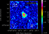
Fig. 2. Wideband image of T CrB obtained from a joint MTMFS deconvolution of all our ALMA 12 m array data on the target (bands 1 – 8) from 2024 as listed in Table 1. The size of the synthesized beam (angular resolution) is given by the ellipse plotted in the lower left corner. The parameters (major axis, minor axis, and position angle) are 1.62 arcsec, 1.16 arcsec, and 19.8°, respectively. The image resembles that of the PSF. The object is detected with 15σ significance but there are no resolved spatial features. ALMA was tracking the object at all times taking into account its proper motion. The spatial coordinates shown are those for 10 August 2024, the start of the observations.
-
Using only bands 7 and 8 to maximize angular resolution (Figs. 3 and 4). See Section 4.
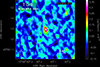
Fig. 3. Continuum image obtained from combining only our band 7 and 8 observations of T CrB where we achieve the best angular resolution. The two magenta circles represent the boundaries of an annulus around the position of T CrB with inner radius 0.8 arcsec (twice the angular resolution of the observation) and outer radius 1.6 arcsec, inside which we derive an upper limit on diffuse emission in the circumbinary medium.
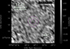
Fig. 4. Image from the peak channel of SPW 4 in our complete ALMA band 7 observations of the region around T CrB in 2024 (see Table 2), where we achieve the best angular resolution and sensitivity for an individual line. This SPW is centered (in LSRK) on the rest frequency of HCN v = 0 J = 4–3 line. The radio velocity shown in the upper right is relative to this line. The image is consistent with pure noise. The signal, for which this image shows the peak channel, is extracted from the annulus given by the two magenta circles around the image center, which are the same as in Fig. 3. The beam major and minor axes are 0.48 arcsec and 0.30 arcsec. We show this image in gray scale to draw attention the fact that this is a narrow-band image of a single spectral channel.
In order to obtain per-band/per visit images of the target, we produced MTMFS images from the combination of all target data from one MOUS using the CASA tclean task with standard ALMA QA parameters, in particular using deconvolver “mtmfs” (with nterms = 2 where the fractional bandwidth is > 10%), and Briggs weighting with robust = 0.5. All images show a central emission compatible with a point-source after deconvolution (“clean”) using a tight elliptical mask around the image center (the image resembles the point spread function (PSF) of the interferometer). A few iterations and one major cycle suffice to obtain a noise-like residual. We obtained the final estimate of the noise RMS from an annulus in the non-primary-beam-corrected image between around 30% and 60% of the primary beam radius around the image center. The flux density of the target was obtained by fitting a Gaussian to an elliptical region of the size of the synthesized beam around the peak emission (which we find to be within a synthesized beam radius of the image center, the nominal position of T CrB1). The pixel width was chosen to be 10% of the minor axis of the synthesized beam size (see column “beam” in Table 1). The flux density was then taken as the peak of the fit Gaussian. Table 3 shows the resulting flux densities together with the centroid time (MJD) and frequency of the observation. Also shown is the orbital phase of T CrB (according to Fekel et al. 2000) corresponding to the time centroid. This phase is based on the radial velocity of the M giant in the binary and defined to be zero when the radial velocity is maximal.
4. Spectral and spatial analysis
The spectrum of T CrB at millimeter wavelengths in quiescence, long after a thermonuclear explosion has taken place on the WD, is expected to be time-dependent on scales of days or weeks for two main reasons. First, the emission is a composite of the emission from near the WD accretion disk, the emission from the red giant, and the emission from its wind (which is mostly free-free emission by the ionized part of the wind). Due to the rotation of the binary system with orbital period 227.6 days, these three origins of emission are seen in different projections, and they partially occult each other (the inclination of the system is between 49° and 56° according to the latest analysis by Hinkle et al. 2025). This leads to significant variations in the object’s apparent brightness without any intrinsic changes in the physical processes in the binary system. For example the recent Cousins I (800 ± 150 nm) light curve of T CrB, which can be obtained from the AAVSO database (Kloppenborg 2025), has a near-sinusoidal shape with a period of half the orbital period of T CrB and an amplitude (in flux density) of around 30% of the maximum flux density. We must assume that also the emission at millimeter wavelengths is modulated by the binary’s rotation, not necessarily with the same relative amplitude as in the optical, but with the same period. And if the amplitude of the modulation is wavelength-dependent, this results in a modulation of the spectral shape.
The second main reason for expecting the millimeter emission of T CrB to have a variable spectrum is that the accretion rate onto the WD is variable leading to moderate high states that have been studied, as was mentioned in the introduction, at multiple wavelengths, also by Linford et al. (2019, hereafter L2019) in the frequency window just below that of ALMA at 5 GHz to 35 GHz.
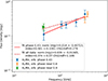 |
Fig. 1. Our 2024 ALMA T CrB flux density measurements from Table 3 plotted vs. centroid frequency and coloured by orbital phase (see legend). The error bars include the systematic errors. The solid line shows a power law fit to the points for orbital phase 0.43, while the dashed line shows a power law fit to all points. |
Our pre-burst observations of T CrB span nearly half a rotation of the system (46% from phase 0.4328 to 0.8889) but we are far from having a complete coverage of all bands at all orbital phases. We only have one nearly complete set of observations at phase 0.43 with bands 1, 3, 4, 6, and 7. Figure 1 shows a power-law fit (solid line) to these five flux density measurements we have at near-equal phase (see also Table 3). Super-imposed, but not included in the fit, are the remaining measurements from Table 3 which were made at other orbital phases. If we include all nine measurements in the fit, we obtain the dashed line. The best fit parameters are given in Table 4. All fits were performed under Python 3 using the “curve_fit” function from the scipy.optimize package (see https://scipy.org).
While the reduced χ2 of 1.1 for the power law fit to all data points is perfectly acceptable, and the spectral index is formally better constrained when all data are used, we note that due to the well-motivated expectation of spectral variability, only our spectrum for phase 0.43 can be regarded as well defined because our dataset lacks spectral coverage at other phases. However, due to the faintness of the target, both spectra are still marginally consistent.
To help constrain the spectrum further and at the same time look for potential signs of extended structure (our observations in bands 6 – 8 have angular resolutions better than 0.5 arcsec), we combined all our ALMA 12 m array data and imaged it using CASA tclean with deconvolver MTMFS with two Taylor terms (nterms = 2) such that in addition to a high-resolution image, we also obtained an estimate of the best fit power law spectral index of the object. The resulting image is shown in Fig. 2. It is in good agreement with the PSF of the dataset, and thus there is no indication of any resolved spatial features.
The image deconvolution is unproblematic and converges quickly. The achieved noise RMS is 0.018 mJy/beam, the peak flux density is 0.258 mJy/beam, and the centroid frequency of the observation is 223.468 GHz. The spatial century coordinates of the image were chosen to be those for the start of the observation on 10 August 2024. ALMA was, however, tracking the object at all times taking into account its proper motion, so the image center coincides with the nominal position of T CrB. Fitting a Gaussian to the emission results in a peak position that is inside the central pixel, confirming the correctness of the ephemeris of T CrB within the angular resolution. Also in all individual per-band images, the peak position was less than a beam radius away from the image center.
The primary-beam-corrected “alpha” and “alpha.error” images (spectral index, α, and corresponding error estimate) produced by the MTMFS deconvolution contain in their central pixels (where also the peak flux density is measured) the value α = 0.57 ± 0.23, which is in very good agreement with our measurement in Table 4, albeit with a larger uncertainty.
The gas content of the circumbinary region of T CrB is best constrained by our band 7 and 8 observations because here we achieve the best angular resolution. In the combined image from all our band 7 and 8 data, the beam full-width-at-half-maximum major and minor axes are 0.48 arcsec and 0.35 arcsec, 0.42 arcsec on average (Fig. 3). In an annulus of 0.8 arcsec (= twice the angular resolution to avoid any residual sidelobes of the PSF) inner radius and 1.6 arcsec outer radius centered on T CrB (equivalent to 720 AU – 1440 AU at the distance of T CrB based on Gaia DR3 data (Bailer-Jones et al. 2021)), we obtain a mean surface brightness of 4.2 μJy/beam and an RMS of 43.7 μJy/beam. This means there is no significant continuum emission between ca. 344 GHz and 407 GHz down to a surface brightness of 0.09 mJy/beam with a confidence level of 2σ. With the given beam size, this corresponds to a brightness temperature upper limit in the annulus of Tb < 4.7 K.
The line emission in this spectral and spatial region is best constrained in band 7 (7 and 7b combined), SPW 4 (velocity resolution 0.82 km/s, see also Table 2). The most prominent potential line in this window is the tracer HCN v = 0 J = 4–3 with a rest frequency near 354.5055 GHz. Neither this nor any other line is detected. Even if the frequency of the line was shifted differently at different orbital periods (since we combine 7 and 7b with corresponding orb. phases 0.43 and 0.59), any upper limit on the HCN line emission must be ≤ that obtained from the channel with the brightest signal. We thus obtained a 2σ upper limit on the line surface brightness (assuming a 10 km/s line width) for any potential line in SPW 4 from the peak channel of that SPW with a value of 3.1 mJy/beam. There is no indication of any spatial structure. The images of the peak and all other channels look like noise (Fig. 4).
5. Spectral reanalysis of the 2016-2017 VLA data
Since our ALMA data is the first measurement of T CrB at frequencies between 42 GHz and 407 GHz, we cannot make statements about long-term variability in this regime. We can, however, assume a smooth spectral transition to the frequency window just below ours and compare to the measurements made by L2019 in 2016-2017 with the VLA at 5 GHz to 35 GHz.
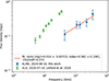 |
Fig. 5. Comparison of our ALMA spectrum of T CrB for orbital phase 0.43 from 10 August 2024 (blue points) with a representative spectrum of the same object observed on 14 July 2016 with the VLA by Linford et al. (2019) (green circles). The fit parameters given in the caption are those of a power law fit to our points as is also shown in Fig. 1. |
Figure 5 shows our spectrum for phase 0.43 (August 2024) together with a representative spectrum from L2019 for the date 14 July 2016 where they have a complete set of data points over their full frequency range. In 2016-2017, T CrB was in a high state, and (as one can see from Fig. 5 by extrapolating our spectrum down in frequency by a few GHz) approximately a factor of 5 brighter around 35 GHz than it was in the second half of 2024 when ALMA observed it. The decrease in brightness at IR or visible wavelengths between 2017 and 2024 was much more modest (ca. 0.5 mag corresponding to a factor 1.58) according to the AAVSO database (Kloppenborg 2025). Furthermore, the T CrB spectrum from 2016-2017 with an average index of 1.0 ± 0.03 (from 5 GHz to 35 GHz, averaging over values given by L2019 for all their individual nights) was significantly harder than our spectrum with index 0.56 ± 0.11 (also shown in Fig. 5).
A closer look at the seven individual spectra presented by L2019 for their different visits to T CrB in 2016-2017 reveals that the spectra may have some curvature. L2019 do not mention the goodness of their power-law fits but if we re-fit their four points above 13.5 GHz in each of their spectra with a separate power law, we find that in all cases except two, the fit is good and results in an index between 0.82 and 1.0. The exceptions are the nights of 25 August 2016 and 22 September 2016, where the obtained index is much lower (0.29 and 0.51, respectively) with a worse goodness of fit. Inspecting the “Observations” section of L2019, one finds on pages 2 and 3 of the paper that (a) the two points from August and September 2016 were the only ones for which the VLA atmospheric delay model “caused issues with source location and smearing along the direction of elevation” (although L2019 argued that the atmospheric delay model issue did not affect their measurements). (b) The above effect was larger for higher frequencies. (c) The 29.5 GHz and 35 GHz points for these two months were “found to be decorrelated.” The checksource was used to derive a correction to the flux density. The error bars of the measurements were “increased accordingly.” We interpret this as a justification to exclude the two observing nights from the sample. They obviously are affected by systematic errors, which make them not useful for our investigation of the variability of the spectral index.
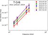 |
Fig. 6. The VLA data points from Linford et al. (2019) used by us to derive the spectral indices in Table 5. The lines show our power law fits. |
Results from our power-law fits to the upper four points (13.5 GHz to 35 GHz) of the per-visit spectra of T CrB by Linford et al. (2019) observed with the VLA in 2016-2017.
Table 5 lists our fit results for the L2019 data between 13.5 GHz and 35 GHz on the five nights with good, comparable data (also shown in Fig. 6). The average spectral index for these nights is 0.90 ± 0.02 (13.5 GHz – 35 GHz) compared to the average spectral index of 0.96 ± 0.03 measured by L2019 over their full spectral range of 5 GHz to 35 GHz for the same nights.
Comparing the different spectral indices obtained from the VLA data from 2016-2017 in the spectral range just below ours with the spectral index obtained from our observations in 2024, we can say that T CrB very likely had a softer spectrum around 40 GHz in 2024 than it had at any time during the VLA observations. However, the difference between the softest VLA index and ours is only 0.26 ± 0.13, a 2 sigma effect. Deeper observations covering the entire orbital period would be needed to draw firmer conclusions. Compared to the average VLA index we measure between 13.5 and 35 GHz (see above), our ALMA index is softer by 0.34 ± 0.11.
6. Discussion
6.1. Model
In order to interpret the VLA and ALMA spectra, we work with the simplified model inherited from Panagia & Felli (1975) and Wright & Barlow (1975): an isotropic, isothermal, fully ionized, and free-free emitting stellar wind. The radiation from the WD and its accretion disk are responsible for the anomalously high wind ionization and temperature compared to an isolated red giant star. Yet, we assume the wind temperature, T0, to be uniform and discard geometrical effects such as the ones considered by Taylor & Seaquist (1984).
The wind number density profile, n(r), was set to a power law:
 (1)
(1)
with β > 0 the density profile index, a dimensionless constant, R the stellar radius, and n0 the number density scale. In these conditions, there is a critical frequency, νt, called the turnover frequency, above which the wind is fully optically thin. The behavior of the flux density, Sν, is twofold, depending on whether ν ≫ νt (optically thin regime) or ν < νt (optically thin and thick hybrid regime).
In the frequency range, we span (5 GHz to 400 GHz) and for realistic wind temperatures (T0 > 104 K, such that the fully ionized hypothesis holds), we can make the Rayleigh-Jeans approximation (hν ≪ kBT0) and use a simplified form of the free-free opacity in order to derive analytical expressions. In these conditions, the spectral index, α, of the free-free emission of the wind is ∼ − 0.1 in the optically thin regime. In the hybrid regime, below the turnover frequency, the spectral index, α, is uniquely set by the exponent, β, in equation (1) through
 (2)
(2)
such that a wind at uniform speed (which means β = 2 from mass conservation) produces a spectral index of α ∼ 0.6. However, since the wind steadily accelerates from the dust condensation radius (the distance from the star where the temperature is low enough for dust grains to form and couple to the underlying continuum, Höfner & Olofsson 2018), we expect β > 2, at least up to a distance where the wind has reached its terminal speed. This means that accounting for wind acceleration yields a steeper spectrum, with α > 0.6.
In radio/millimeter, an accurate estimate of the turnover frequency can be obtained from the implicit equation:
 (3)
(3)
where
 (4)
(4)
and fg is the Gaunt factor, a slowly varying function of ν given by van Hoof et al. (2014)
 (5)
(5)
Therefore, once the exponent, β, has been obtained from the spectral index in the hybrid regime, a measure of the turnover frequency provides a relation between n0, R, and T0.
Finally, the norm, K, of the spectral fit in the hybrid regime is given by
![Mathematical equation: $$ \begin{aligned} K\sim \pi \left[\frac{I(\beta )}{3}\right]^{\frac{2}{2\beta -1}}\frac{\Sigma (\beta )}{D^2\nu _0^{\alpha }}B_{\nu _0}(T_0)n_0^{\frac{4}{2\beta -1}}R^{2+\frac{2}{2\beta -1}}\chi _{\nu _0}(T_0)^{\frac{2}{2\beta -1}} ,\end{aligned} $$](/articles/aa/full_html/2025/10/aa55830-25/aa55830-25-eq8.gif) (6)
(6)
where D is the distance to the source, ν0 is a frequency representative of the frequency range. The exact choice of ν0 has only a minor impact on the results, and so we set it to 30 GHz, essentially the geometric mean of the VLA-ALMA frequency range. Bν(T) is the Planck function. Σ(β) is a series given by
 (7)
(7)
and χν(T) is given by
 (8)
(8)
 (9)
(9)
(in CGS units), with κff the free-free opacity. Therefore, if we know the distance, D, and the exponent, β, the norm, K, provides a second relation between n0, R, and T0.
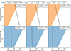 |
Fig. 7. Possible values of red giant wind particle number density scale and plasma temperature (n0, T0) (solid lines) for the 2016 VLA (top panels) and 2024 ALMA spectra (bottom) of T CrB, for an assumed stellar radius of R = 54 R⊙ (left), R = 70 R⊙ (middle), and R = 100 R⊙ (right). The regions allowed by the lower limit on the turnover frequency are in white. Inside the shaded regions, the lines of (n0, T0) solutions are shown as dashed in order to indicate that they do not respect the constraint set by the lower limit on the turnover frequency and are thus not physical. The top axis indicates stellar mass-loss rates corresponding to the number density, n0. A fiducial frequency, ν0 = 30 GHz, whose choice little alters the result compared to other systematics, was used to compute T0(n0) from equation (6). |
6.2. Data interpretation
The spectral indices we find for the ALMA and VLA data (Tables 4 and 5) are all incompatible with the fully optically thin regime. While there is a suggestion of some curvature in the VLA spectra, we do not see a significant break that would suggest that the turnover frequency is well inside our frequency range. Hereafter, we set a lower limit to the turnover frequency to the last data point of each dataset:
 (10)
(10)
 (11)
(11)
and we interpreted this data in the hybrid regime (ν < νt). With equation (2) and the spectral indices we fit, we deduced:
 (12)
(12)
 (13)
(13)
To derive the uncertainty estimates given in (12) and (13), we solved equation (2) for β and then propagated the uncertainty values of spectral index α from Tables 4 and 5, respectively, into an uncertainty of the corresponding β. The derived uncertainties of the β values do not include systematics arising from the simplifying assumptions of the model (e.g., assuming a power law for the wind density profile). These systematics would probably dominate but are not random and would shift both derived values of β in the same direction. So while the absolute values of β are quite uncertain, we can argue that they are different by more than 3σ, meaning that the underlying wind dynamics were different in the two time periods, with a more accelerating wind in 2016 – 2017, and a more uniform wind speed profile from its basis during our 2024 observations.
Since this data spans the hybrid regime, we only have the lower limits on the turnover frequency, νt, which translate into lower limits for n0 and R, and an upper limit for T0. Then, equation (3) delimits a range of possible triplets (n0, R, T0).
Next, we used equation (6) to obtain a relation between n0, R, and T0, knowing β and using the distance, D∼895 pc (Bailer-Jones et al. 2021). From the spectral type of the donor star, which is approximately M2 III to M4.5 III (Yudin & Munari 1993; Mürset & Schmid 1999; Munari et al. 2016; Zamanov et al. 2023), and from arguments related to mass transfer through Roche lobe overflow (Zamanov et al. 2023, 2024; Planquart et al. 2025), we expect a stellar radius ranging between 70 and 100 R⊙ according to the evolutionary tracks by Straizys & Kuriliene (1981). The latest analysis by Hinkle et al. (2025) suggests, however, that a radius of 63.4 R⊙ is more correct (assuming the Gaia DR3 distance), or an even lower value of 54 R⊙ if the distance is made a fit parameter (see introduction). We plot the relation T0(n0) from K for the two extreme potential values of R and for 70 R⊙, and we retain only the values that match the constraint from the corresponding turnover frequency’s lower limit.
The results are shown in Figure 7, where allowed values lie in the white regions. In the top x axis, we provide an estimate of the stellar mass-loss rate assuming a wind launched at 10 km/s from the stellar surface (and neglecting the inherent inconsistencies due to β > 2). We see that for the 2016-2017 VLA data, this model gives a range of possible values. The stellar mass loss rate we measure is in the range of 1 to 5 × 10⁻⁸ M⊙/yr, in agreement with the expected values from the accretion rate during the high state (Stanishev et al. 2004) and from the recurrence period of the nova (Schaefer 2023b). However, the 2024 ALMA data cannot be interpreted with this model. Indeed, the flux is too low and the turnover frequency too high to yield a range of possible values for n0 and T0, for any realistic stellar radius, R. The line of possible (T0, n0) values is fully inside the excluded region in the three lower plots in Fig. 7. We think that this is due to the low activity of the system in 2024 compared to 2016-2017, which would mean that the ionizing flux from the accretion disk was much lower and only a small fraction of the stellar wind, centered on the WD, was sufficiently ionized to radiate through free-free emission.
7. Conclusions
We analyzed our ALMA 2024 T CrB data and for comparison VLA 2016-2017 data by Linford et al. (2019) in order to determine the properties (density, temperature, and ionization) of the stellar wind in which the upcoming nova will take place. We find that the spectral index above 35 GHz in 2024 is significantly lower than the index measured just below 35 GHz in 2016-2017. But in both cases the index is well above the optical thin regime (−0.1). So, both in 2016-2017 and in 2024, the turnover frequency, νt, above which the wind becomes fully optically thin, was well above 35 GHz, and in 2024 it was even above 350 GHz. It is unlikely that the spectrum at ALMA energies was the same in 2016-2017 and in 2024, because it would not fit the expected shape of the turnover, which should happen within a decade of frequency. What we see at ALMA energies, however, is consistent with a straight power law from 40 GHz to 400 GHz. We conclude that the overall state of the object and its wind must have been very different in 2016-2017 and 2024, and the spectra of the two states are not just scaled versions of each other with different intensity scales.
We showed that the VLA 2016-2017 data can be well explained by radio free-free emission from an isotropic, isothermal, and fully ionized wind associated with a stellar mass loss rate of ∼10−8 M⊙/yr. However, this model is unable to account for the ALMA 2024 low flux and high turnover frequency, which suggests that a more complex model (beyond the scope of this paper) needs to be employed for the 2024 state involving an only partially ionized wind. This is in agreement with the reported end of the super-active phase in early 2023 (Munari 2023).
Our aggregate bandwidth images of the object in all ALMA bands are consistent with that of a point source. The most stringent limit on the presence of matter in the space near the object is achieved in bands 7 and 8 with a continuum sensitivity of 0.09 mJy/beam limiting the brightness temperature near 374 GHz to Tb < 4.7 K in a 720 AU to 1440 AU annulus (assuming the Gaia DR3 distance) around T CrB. The emission observed from the central point source is constrained to an angular radius of 0.4 arcsec (corresponding to 360 AU assuming the same distance). No line emission is detected in any band.
In future ALMA observations of the quiescent state of T CrB and similar objects, the turnover frequency could be further constrained by extending the concurrent frequency coverage (within a few days) into band 9 and doubling the flux sensitivity.
The T CrB position used was (ICRS) RA 15:59:30.154, Dec +25.55.12.909 (Epoch 2025-08-10, 22:40:20.4 UT), with proper motion in RA = −6.853E-16 rad/s, in Dec = 1.846E-15 rad/s in agreement with the values from Gaia Collaboration (2020).
Acknowledgments
This paper makes use of the following ALMA data: ADS/JAO.ALMA#2023.A.00038.T, ADS/JAO.ALMA#2023.A.00041.S. ALMA is a partnership of ESO (representing its member states), NSF (USA) and NINS (Japan), together with NRC (Canada), NSTC and ASIAA (Taiwan), and KASI (Republic of Korea), in cooperation with the Republic of Chile. The Joint ALMA Observatory is operated by ESO, AUI/NRAO and NAOJ. GS acknowledges support by the Spanish MINECO grant PID2023-148661NB-I00, by the E.U. FEDER funds, and by the AGAUR/Generalitat de Catalunya grant SGR-386/2021. GS acknowledges support from the Max-Planck-Institut für extraterrestrische Physik for her visit in summer 2024, when fruitful discussions about T CrB and ALMA with the coauthors gave rise to the present work. IEM acknowledges support from the grant ANID FONDECYT 11240206 and funding via the BASAL Centro de Excelencia en Astrofisica y Tecnologias Afines (CATA) grant PFB06/2007. We acknowledge useful discussions with Steven N. Shore (Universitá de Pisa) and the anonymous referee.
References
- Acciari, V. A., Ansoldi, S., Antonelli, L. A., et al. 2022, Nat. Astron., 6, 689 [NASA ADS] [CrossRef] [Google Scholar]
- Azzollini, A., Shore, S. N., & Kuin, P. N. 2022, Res. Notes Am. Astron. Soc., 6, 92 [Google Scholar]
- Azzollini, A., Shore, S. N., Kuin, P. N., & Page, K. L. 2023, A&A, 674, A139 [NASA ADS] [CrossRef] [EDP Sciences] [Google Scholar]
- Bailer-Jones, C. A. L., Rybizki, J., Fouesneau, M., Demleitner, M., & Andrae, R. 2021, AJ, 161, 147 [Google Scholar]
- CASA Team, Bean, B., Bhatnagar, S., et al. 2022, PASP, 134, 114501 [NASA ADS] [CrossRef] [Google Scholar]
- Cortes, P. C., Vlahakis, C., Hales, A., et al. 2024, ALMA Technical Handbook Cycle 11 (ALMA Doc. 11.3, ver. 1.4) https://almascience.eso.org/documents-and-tools/cycle11/alma-technical-handbook [Google Scholar]
- Darnley, M. J. 2021, in The Golden Age of Cataclysmic Variables and Related Objects V, 2, 44 [Google Scholar]
- de Ruiter, I., Nyamai, M. M., Rowlinson, A., et al. 2023, MNRAS, 523, 132 [NASA ADS] [CrossRef] [Google Scholar]
- Fekel, F. C., Joyce, R. R., Hinkle, K. H., & Skrutskie, M. F. 2000, AJ, 119, 1375 [NASA ADS] [CrossRef] [Google Scholar]
- Gaia Collaboration, 2020, Gaia EDR3 (CDS/ADC Collection of Electronic Catalogues), 1350 [Google Scholar]
- Hinkle, K. H., Nagarajan, P., Fekel, F. C., et al. 2025, ApJ, 983, 76 [Google Scholar]
- Hjellming, R. M., van Gorkom, J. H., Taylor, A. R., et al. 1986, ApJ, 305, L71 [NASA ADS] [CrossRef] [Google Scholar]
- Höfner, S., & Olofsson, H. 2018, A&A Rev., 26, 1 [CrossRef] [Google Scholar]
- Hunter, T. R., Indebetouw, R., Brogan, C. L., et al. 2023, PASP, 135, 074501 [NASA ADS] [CrossRef] [Google Scholar]
- José, J. 2016, Stellar Explosions: Hydrodynamics and Nucleosynthesis (CRC Press) [Google Scholar]
- José, J., & Hernanz, M. 1998, ApJ, 494, 680 [Google Scholar]
- Kato, M., & Hachisu, I. 2012, Bull. Astron. Soc. India, 40, 393 [NASA ADS] [Google Scholar]
- Kloppenborg, B. 2025, Observations from the AAVSO International Database, https://www.aavso.org [Google Scholar]
- Linford, J. D., Chomiuk, L., Sokoloski, J. L., et al. 2019, ApJ, 884, 8 [NASA ADS] [CrossRef] [Google Scholar]
- López-Coto, R., Sitarek, J., Bednarek, W., et al. 2015, in 34th International Cosmic Ray Conference (ICRC2015), Int. Cosmic Ray Conf., 34, 731 [Google Scholar]
- Munari, U. 2023, Res. Notes Am. Astron. Soc., 7, 145 [Google Scholar]
- Munari, U. 2025, Contrib. Astron. Obs. Skalnate Pleso, 55, 47 [Google Scholar]
- Munari, U., Dallaporta, S., & Cherini, G. 2016, New A, 47, 7 [Google Scholar]
- Munari, U., Giroletti, M., Marcote, B., et al. 2022, A&A, 666, L6 [NASA ADS] [CrossRef] [EDP Sciences] [Google Scholar]
- Mürset, U., & Schmid, H. M. 1999, A&AS, 137, 473 [NASA ADS] [CrossRef] [EDP Sciences] [Google Scholar]
- Nayana, A. J., Anupama, G. C., Roy, N., et al. 2024, MNRAS, 528, 5528 [NASA ADS] [CrossRef] [Google Scholar]
- O’Brien, T. J., Bode, M. F., Porcas, R. W., et al. 2006, Nature, 442, 279 [CrossRef] [Google Scholar]
- Orlando, S., Drake, J. J., & Laming, J. M. 2009, A&A, 493, 1049 [NASA ADS] [CrossRef] [EDP Sciences] [Google Scholar]
- Panagia, N., & Felli, M. 1975, A&A, 39, 1 [Google Scholar]
- Planquart, L., Jorissen, A., & Van Winckel, H. 2025, A&A, 694, A85 [NASA ADS] [CrossRef] [EDP Sciences] [Google Scholar]
- Rau, U., & Cornwell, T. J. 2011, A&A, 532, A71 [NASA ADS] [CrossRef] [EDP Sciences] [Google Scholar]
- Rupen, M. P., Mioduszewski, A. J., & Sokoloski, J. L. 2008, ApJ, 688, 559 [NASA ADS] [CrossRef] [Google Scholar]
- Schaefer, B. E. 2023a, MNRAS, 524, 3146 [NASA ADS] [CrossRef] [Google Scholar]
- Schaefer, B. E. 2023b, J. Hist. Astron., 54, 436 [CrossRef] [Google Scholar]
- Shafter, A. W. 2017, ApJ, 834, 196 [CrossRef] [Google Scholar]
- Shore, S. N. 2008, in RS Ophiuchi (2006) and the Recurrent Nova Phenomenon, eds. A. Evans, M. F. Bode, T. J. O’Brien, & M. J. Darnley, ASP Conf. Ser., 401, 19 [Google Scholar]
- Shore, S. N., & Aufdenberg, J. P. 1993, ApJ, 416, 355 [NASA ADS] [CrossRef] [Google Scholar]
- Sokoloski, J. L., Luna, G. J. M., Mukai, K., & Kenyon, S. J. 2006, Nature, 442, 276 [CrossRef] [Google Scholar]
- Sokoloski, J. L., Rupen, M. P., & Mioduszewski, A. J. 2008, ApJ, 685, L137 [NASA ADS] [CrossRef] [Google Scholar]
- Stanishev, V., Zamanov, R., Tomov, N., & Marziani, P. 2004, A&A, 415, 609 [NASA ADS] [CrossRef] [EDP Sciences] [Google Scholar]
- Starrfield, S., Iliadis, C., & Hix, W. R. 2016, PASP, 128, 051001 [Google Scholar]
- Starrfield, S., Bose, M., Woodward, C. E., et al. 2025, ApJ, 982, 89 [Google Scholar]
- Straizys, V., & Kuriliene, G. 1981, Ap&SS, 80, 353 [CrossRef] [Google Scholar]
- Taylor, A. R., & Seaquist, E. R. 1984, ApJ, 286, 263 [Google Scholar]
- Townsley, D. M. 2008, in RS Ophiuchi (2006) and the Recurrent Nova Phenomenon, eds. A. Evans, M. F. Bode, T. J. O’Brien, & M. J. Darnley, ASP Conf. Ser., 401, 131 [Google Scholar]
- van Hoof, P. A. M., Williams, R. J. R., Volk, K., et al. 2014, MNRAS, 444, 420 [Google Scholar]
- Walder, R., Folini, D., & Shore, S. N. 2008, A&A, 484, L9 [NASA ADS] [CrossRef] [EDP Sciences] [Google Scholar]
- Wright, A. E., & Barlow, M. J. 1975, MNRAS, 170, 41 [Google Scholar]
- Yudin, B., & Munari, U. 1993, A&A, 270, 165 [Google Scholar]
- Zamanov, R., Boeva, S., Latev, G. Y., et al. 2023, A&A, 680, L18 [NASA ADS] [CrossRef] [EDP Sciences] [Google Scholar]
- Zamanov, R. K., Stoyanov, K. A., Marchev, V., et al. 2024, Astron. Nachr., 345, e20240036 [NASA ADS] [CrossRef] [Google Scholar]
All Tables
Results from our power-law fits to the upper four points (13.5 GHz to 35 GHz) of the per-visit spectra of T CrB by Linford et al. (2019) observed with the VLA in 2016-2017.
All Figures
|
Fig. 2. Wideband image of T CrB obtained from a joint MTMFS deconvolution of all our ALMA 12 m array data on the target (bands 1 – 8) from 2024 as listed in Table 1. The size of the synthesized beam (angular resolution) is given by the ellipse plotted in the lower left corner. The parameters (major axis, minor axis, and position angle) are 1.62 arcsec, 1.16 arcsec, and 19.8°, respectively. The image resembles that of the PSF. The object is detected with 15σ significance but there are no resolved spatial features. ALMA was tracking the object at all times taking into account its proper motion. The spatial coordinates shown are those for 10 August 2024, the start of the observations. |
| In the text | |
|
Fig. 3. Continuum image obtained from combining only our band 7 and 8 observations of T CrB where we achieve the best angular resolution. The two magenta circles represent the boundaries of an annulus around the position of T CrB with inner radius 0.8 arcsec (twice the angular resolution of the observation) and outer radius 1.6 arcsec, inside which we derive an upper limit on diffuse emission in the circumbinary medium. |
| In the text | |
|
Fig. 4. Image from the peak channel of SPW 4 in our complete ALMA band 7 observations of the region around T CrB in 2024 (see Table 2), where we achieve the best angular resolution and sensitivity for an individual line. This SPW is centered (in LSRK) on the rest frequency of HCN v = 0 J = 4–3 line. The radio velocity shown in the upper right is relative to this line. The image is consistent with pure noise. The signal, for which this image shows the peak channel, is extracted from the annulus given by the two magenta circles around the image center, which are the same as in Fig. 3. The beam major and minor axes are 0.48 arcsec and 0.30 arcsec. We show this image in gray scale to draw attention the fact that this is a narrow-band image of a single spectral channel. |
| In the text | |
|
Fig. 1. Our 2024 ALMA T CrB flux density measurements from Table 3 plotted vs. centroid frequency and coloured by orbital phase (see legend). The error bars include the systematic errors. The solid line shows a power law fit to the points for orbital phase 0.43, while the dashed line shows a power law fit to all points. |
| In the text | |
|
Fig. 5. Comparison of our ALMA spectrum of T CrB for orbital phase 0.43 from 10 August 2024 (blue points) with a representative spectrum of the same object observed on 14 July 2016 with the VLA by Linford et al. (2019) (green circles). The fit parameters given in the caption are those of a power law fit to our points as is also shown in Fig. 1. |
| In the text | |
|
Fig. 6. The VLA data points from Linford et al. (2019) used by us to derive the spectral indices in Table 5. The lines show our power law fits. |
| In the text | |
|
Fig. 7. Possible values of red giant wind particle number density scale and plasma temperature (n0, T0) (solid lines) for the 2016 VLA (top panels) and 2024 ALMA spectra (bottom) of T CrB, for an assumed stellar radius of R = 54 R⊙ (left), R = 70 R⊙ (middle), and R = 100 R⊙ (right). The regions allowed by the lower limit on the turnover frequency are in white. Inside the shaded regions, the lines of (n0, T0) solutions are shown as dashed in order to indicate that they do not respect the constraint set by the lower limit on the turnover frequency and are thus not physical. The top axis indicates stellar mass-loss rates corresponding to the number density, n0. A fiducial frequency, ν0 = 30 GHz, whose choice little alters the result compared to other systematics, was used to compute T0(n0) from equation (6). |
| In the text | |
Current usage metrics show cumulative count of Article Views (full-text article views including HTML views, PDF and ePub downloads, according to the available data) and Abstracts Views on Vision4Press platform.
Data correspond to usage on the plateform after 2015. The current usage metrics is available 48-96 hours after online publication and is updated daily on week days.
Initial download of the metrics may take a while.