| Issue |
A&A
Volume 702, October 2025
|
|
|---|---|---|
| Article Number | A200 | |
| Number of page(s) | 8 | |
| Section | Stellar structure and evolution | |
| DOI | https://doi.org/10.1051/0004-6361/202556201 | |
| Published online | 21 October 2025 | |
The twin red giant branch system BD+20 5391
A case study of low-mass double-core evolution
1
Institut für Physik und Astronomie, Universität Potsdam, Haus 28, Karl-Liebknecht-Str. 24/25, 14476 Potsdam, Germany
2
Astronomical Institute AS CR, Fričova 298, 251 65 Ondřejov, Czech Republic
3
Astronomical Institute of the Slovak Academy of Sciences, 059 60 Tatranská Lomnica, Slovakia
4
Institute of Astronomy, KU Leuven, Celestijnenlaan 200D, 3001 Leuven, Belgium
5
Leuven Gravity Institute, KU Leuven, Celestijnenlaan 200D, box 2415, 3001 Leuven, Belgium
6
Thüringer Landessternwarte Tautenburg, Sternwarte 5, 07778 Tautenburg, Germany
7
University of Warwick, Department of Physics, Gibbet Hill Road, Coventry CV4 7AL, UK
⋆ Corresponding author: This email address is being protected from spambots. You need JavaScript enabled to view it.
Received:
1
July
2025
Accepted:
9
August
2025
Abstract
Context. Understanding interactions of binary systems on the red giant branch is crucial to understanding the formation of compact stellar remnants such as helium-core white dwarfs (He-WDs) and hot subdwarfs. However, the detailed evolution of such systems, particularly those with nearly identical components, remains under-explored.
Aims. We aim to analyse the double-lined spectroscopic binary system BD+20 5391, composed of two red giant stars, in order to characterise its orbital and stellar parameters and to constrain its evolution.
Methods. Spectroscopic data were collected between 2020 and 2025 using the Ondřejov Echelle Spectrograph and the Mercator Échelle Spectrograph. The time-resolved spectra were fitted with models to determine the radial velocity curve and derive the system’s parameters. We then used the position of both stars in the Hertzsprung-Russell diagram to constrain the system’s current evolutionary state, and we discuss potential outcomes of future interactions between the binary components.
Results. We find that the two stars in BD+20 5391 will likely initiate Roche lobe overflow (RLOF) simultaneously, leading to a double-core evolution scenario. The stars’ helium core masses at RLOF onset will be almost identical, at 0.33 M⊙. This synchronised evolution suggests two possible outcomes: common envelope ejection, resulting in a short-period double He-WD binary, or a merger without envelope ejection. In the former case, the resulting double He-WD may merge later and form a hot subdwarf star.
Conclusions. This study provides a valuable benchmark example for understanding the evolution of interacting red giant binaries, which will be discovered in substantial numbers in upcoming large-scale spectroscopic surveys.
Key words: binaries: spectroscopic / stars: evolution / stars: low-mass
© The Authors 2025
 Open Access article, published by EDP Sciences, under the terms of the Creative Commons Attribution License (https://creativecommons.org/licenses/by/4.0), which permits unrestricted use, distribution, and reproduction in any medium, provided the original work is properly cited.
This article is published in open access under the Subscribe to Open model. This email address is being protected from spambots. You need JavaScript enabled to view it. to support open access publication.
1. Introduction
Understanding binary stellar evolution is fundamental to our understanding of stellar populations, given that a significant fraction of stars form in binaries or higher-order systems. Of the known F-, G-, and K-type stars, more than 40% reside in multiple-star systems (Duchêne & Kraus 2013; Offner et al. 2023). However, many aspects of binary interaction physics remain poorly understood, even though they can have a profound impact on stellar evolution.
Some stellar classes, such as Be stars (Shao & Li 2014), helium-core white dwarfs (He-WDs; e.g. Li et al. 2019), R Coronae Borealis stars (Clayton 2012), magnetic Ap stars (Ferrario et al. 2009; Tutukov & Fedorova 2010), and hot subdwarfs (sdO/B, Heber 2024), are thought to form exclusively through binary evolution channels. Establishing connections between progenitor systems and their post-interaction products is essential for advancing our understanding of binary interactions and, by extension, stellar evolution.
In low-mass binary systems, significant interaction often begins once one or both components ascend the red giant branch (RGB). If a red giant fills its Roche lobe in a sufficiently wide orbit, stable Roche lobe overflow (RLOF) can strip it to a helium core, yielding a He-WD in a wide binary system (e.g. Iben & Tutukov 1984; Nelemans & Tout 2005), or a hot subdwarf star if helium is ignited. At high mass ratios, the mass transfer is unstable and a common envelope (CE) is formed, which can be ejected and leave a He-WD or sdB remnant in a short-period binary (Han et al. 2002).
In the extreme case that the two stars in a binary system simultaneously evolve into red giants, double-core CE evolution can occur (e.g. Paczynski 1976; Brown 1995; Belczynski & Kalogera 2001; Dewi et al. 2006; Justham et al. 2011). In this scenario, the expanding envelopes of the two stars form a CE as their cores spiral inwards. The parameter space that allows for double-core CE evolution is highly constrained. The two stars must have nearly equal initial masses so that the secondary has already evolved off the main sequence by the time the primary initiates RLOF, which must happen before it reaches the RGB tip (Dewi et al. 2006). In this case, stable mass transfer initially occurs; however, as the secondary expands in response to accretion, it ultimately overfills its Roche lobe and the two stars enter a CE phase simultaneously.
If the envelope is successfully ejected, the result is a compact binary composed of the exposed cores of both stars. Although the double-core CE scenario has not been directly confirmed observationally, compact double-core binaries like the double hot subdwarf system PG 1544+488 (Ahmad et al. 2004; Şener & Jeffery 2014) are known.
Binaries containing two red giant stars of similar mass (‘twin red giants’) are exceedingly rare. Previous research on such objects was focused on oscillating RGB stars (Rawls et al. 2016; Beck et al. 2018, 2022, 2024; Brogaard et al. 2022), but only two – KIC 9163796 (Beck et al. 2018) and KIC 4054905 (Brogaard et al. 2022) – feature components with nearly identical masses. Uzundag et al. (2022) compiled a volume-limited sample of low-mass red giants within 500 pc of the Sun that meet the criteria for potential hot subdwarf progenitors, using data from the second Gaia data release (Gaia DR2; Gaia Collaboration 2018), and conducted follow-up observations of candidates within 200 pc. Benitez-Palacios et al. (2025) expanded on this sample by following up on southern hemisphere candidates within 500 pc. They identified 184 RGB stars, 75 % of which have a high probability of belonging to binary systems with orbital periods of up to 900 days. None of these were identified as double-lined spectroscopic binaries (SB2s) in the Gaia DR3 non-single stars catalogue (Gaia Collaboration 2023a). Although their search was not specifically geared towards detecting SB2s, the absence of such systems in their follow-up spectroscopy is still notable. Eggleton & Yakut (2017) compared binary evolution models to 60 medium- to long-period binaries. Fewer than ten of their systems include two giants on the first giant branch. Finally, large spectroscopic surveys identified thousands of candidate SB2 systems, but only a few are within the red giant selection of Uzundag et al. (2022): about 20 to 30 in the GALAH survey (Traven et al. 2020) and 13 in the APOGEE survey (Kounkel et al. 2021).
In this work we present and analyse a rare instance of a twin red giant – the SB2 BD+20 5391 discovered during a binary red giant survey. It is composed of two giant stars with nearly identical masses and luminosities. This rare configuration provides an excellent opportunity to study binary interactions during the RGB phase.
We aimed to characterise the observational parameters of BD+20 5391 and constrain possible outcomes of its post-interaction evolution, providing a benchmark case for the study of binary interaction in stellar evolution. Section 2 details the observational data and spectra for this system. Section 3 outlines our analysis of the radial velocity curve, spectral fitting, and evolutionary tracks in the Hertzsprung-Russell diagram (HRD). In Sect. 4 we explore potential evolutionary scenarios for this system, including possible binary evolution outcomes. Finally, Sect. 5 summarises our findings and discusses the prospects for future research.
2. Target selection and observations
BD+20 5391 was initially identified as a double-lined system during a search for RGB stars, aimed at finding progenitors of hot subdwarf and He-WD stars, complementing the independent studies of Uzundag et al. (2022) and Benitez-Palacios et al. (2025). Originally using Gaia DR2, we constructed a volume-limited sample of RGB stars just below the red clump within 500 pc of the Sun (see Fig. 1), thus excluding helium-burning giants and mirroring the selection of the 500 pc volume-limited hot subdwarf sample by Dawson et al. (2024). Out of a randomly selected sample of 100 stars located in the northern hemisphere and observable from the Ondřejov Observatory and the Astronomical Institute of the Slovak Academy of Sciences (AISAS) at Skalnaté Pleso, 51 were observed using the high-resolution Ondřejov Echelle Spectrograph (OES; Koubský et al. 2004; Kabáth et al. 2020) mounted on the Perek 2 m Telescope at Ondřejov Observatory, which has a maximum resolving power of R = 51 600 at 5000 Å and a spectral coverage between about 3800 and 8800 Å. The remaining 49 were observed at Skalnaté Pleso Observatory with the 1.3 m telescope and the MUSICOS-style échelle spectrograph (Baudrand & Bohm 1992; Pribulla et al. 2015). BD+20 5391 is the only double-lined system identified in this sample and the focus of this work.
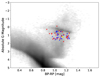 |
Fig. 1. Colour-magnitude diagram of observed red giant stars, based on Gaia DR3 (Gaia Collaboration 2023a). The sample includes RGB stars just below the red clump within 500 pc of the Sun. Blue triangles mark spectra from OES, red circles from AISAS. BD+20 5391 is highlighted in yellow. The grey background marks all Gaia DR3 objects with parallax_over_error > 100 within 500 pc of the Sun. |
Spectroscopic observations of BD+20 5391 were conducted from 2020 to 2025 using the OES, resulting in a total of 15 spectra. Our OES spectra feature an average mean signal-to-noise ratio per pixel of 30 to 35.
We reduced the OES spectra using an Image Reduction and Analysis Facility (IRAF; Tody 1986, 1993) package and a dedicated semi-automatic pipeline1 (Cabezas et al. 2023), which incorporates a full range of standard procedures for échelle spectra reduction: bias correction, flat-fielding, wavelength calibration, heliocentric velocity correction, and continuum normalisation. Additionally, one spectrum was obtained in late 2024 with the High-Efficiency and high-Resolution Mercator Échelle Spectrograph (HERMES; Raskin 2011) at the 1.2 m Mercator Telescope on La Palma, which offers a resolving power of R = 85 000 and a wavelength range from 3800 to 9000 Å, at a median signal-to-noise ratio of 59. The integrated HERMES data reduction pipeline performs standard corrections, robust spectral order tracing and extraction, pre-normalisation, and resampling or merging of spectra described in detail in Raskin (2011).
3. Analysis
Our analysis comprises four complementary methods: spectral analysis, radial velocity modelling, spectral energy distribution (SED) fitting, and HRD fitting to constrain the evolutionary state and future evolution of the system. The details of these methods are outlined in the following sections. Our results are summarised in Table 1.
System- and component-specific parameters.
3.1. Radial velocity curve
As a first step, we used the Interactive Spectral Interpretation System (ISIS; Houck & Denicola 2000) to perform χ2 fits to all spectra. Composite spectral templates were employed to derive the radial velocities of both components in the double-lined spectrum of BD+20 5391. The fitting procedure and model spectra are described in more detail in Sect. 3.2. Table A.1 gives an overview of the radial velocities computed from the spectra of BD+20 5391.
The radial velocities were then modelled assuming an eccentric orbit and fitted using a Markov chain Monte Carlo (MCMC) approach, implemented with the emcee package (Foreman-Mackey et al. 2013) in Python. The resulting radial velocity curves are presented in Fig. 2. We defined the mass ratio as q = MA/MB, where MB refers to the primary component, and MA to the secondary component, with MB > MA.
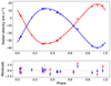 |
Fig. 2. Radial velocity curve of BD+20 5391 for components A (red) and B (blue). Circles show measurements obtained with the OES, and the triangles mark the HERMES measurement. |
The orbital period, P = 80.9 ± 0.5 d, and radial velocity semi-amplitudes KA and KB (see Table 1) are in good agreement with the values reported in the Gaia DR3 non-single star catalogue’s solution (Gaia Collaboration 2023a): PGaia = 81.054 ± 0.028 d, KA,Gaia = 27.7 ± 0.7 km s−1, and KB,Gaia = 27.2 ± 0.7 km s−1. However, the eccentricity derived from our spectra, e = 0.164 ± 0.030, is significantly lower than the Gaia value of eGaia = 0.339 ± 0.016. Since we cannot find a well-matching solution with such a high eccentricity, we conclude that Gaia likely overestimates the eccentricity of this system.
3.2. Spectral analysis
Given the higher resolution and well-defined continuum of the HERMES spectrum, we constrained the atmospheric parameters by performing a χ2 fit using only this spectrum. For this, we computed a grid of ATLAS12/SYNTHE (Kurucz 2013, 1993) models, which use the local thermal equilibrium (LTE) approximation in a 1D geometry. The grid covers a large parameter space in four dimensions: Teff from 3800 to 8000 K in 200 K steps, log g from 5.6 to 1.4 in steps of 0.2, microturbulent velocity ξ (0, 1, 2, 4 km s−1), and metallicity [Fe/H] from −2.5 to 0.5 in steps of 0.5.
Free parameters in the fit included the effective temperatures, radial velocities, and projected rotational velocities of both stars, as well as the surface ratio S = RA2/RB2. Given that the binary system likely formed as a coeval pair, we assumed a common scaled solar metallicity [Fe/H] for both components and no enhancement in alpha-process elements. We further used Newton’s law of gravity g = GM/R2 to impose an additional constraint on the surface gravities of the two components by expressing log gA in terms of log gB:
 (1)
(1)
where q = KB/KA = MA/MB is the mass ratio obtained from the radial velocity curve fit.
An excerpt of our best-fit model fit is shown in Fig. 3, highlighting the clearly resolved contributions of both stars. The derived atmospheric parameters are presented in Table 1.
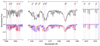 |
Fig. 3. Selected ranges in the double-lined HERMES spectrum of BD+20 5391. The upper section shows the observed data in light grey and the combined model fit as a dashed black line, while the lower part displays the contributions of the individual components, offset by −0.5 for clarity. Component A is shown in red, component B in blue; strong lines are labelled. |
To account for deficiencies in our model, such as the use of the LTE and 1D approximations, we assumed systematic uncertainties of ± 50 K to Teff and 0.1 to log g for the parameters derived from the spectral fit, which is roughly consistent with the study of Blanco-Cuaresma (2019, Fig. 8) for grid-based model fits. For ξ and v sin i we assumed uncertainties of 0.1 and 0.2, respectively, since the impact of statistical errors is negligible due to the high S/N and large number of data points in the HERMES spectrum. We note that the binary nature of BD+20 5391 may introduce additional uncertainties that are difficult to quantify. However, since both components are well resolved in the high-quality HERMES spectra, these uncertainties remain statistically small.
3.3. Spectral energy distribution
To constrain the stellar parameters of both components, we combined the spectroscopic parameters with the Gaia parallax (Lindegren et al. 2021) and the observed SED, as constructed from photometric measurements. Our SED fitting method is described in detail by Heber et al. (2018).
Here we performed a χ2 minimisation to obtain the best-fit angular diameter (Θ). The spectral fit parameters ξ, [Fe/H], log gA, log gB, Teff,A, Teff,B, and the surface ratio (S) were treated as fixed inputs.
In the fitting procedure, we accounted for reddening using the extinction law of Fitzpatrick et al. (2019), with an extinction parameter R55 = 3.02, which is standard for the Galaxy’s diffuse interstellar medium. To limit the number of free parameters, we fixed the monochromatic colour excess to a value of E(44−55) = 0.06 mag, based on the estimates provided by the Schlegel et al. (1998), Schlafly & Finkbeiner (2011), Capitanio et al. (2017), and Green et al. (2019) reddening maps. Our model predicts a marginally higher near-ultraviolet flux compared to the observed values from Gaia, which may be caused by limitations in the SYNTHE model used for the spectral fit.
To obtain the stellar radius,
 (2)
(2)
the angular diameter was then combined with the parallax ϖ = 2.341 ± 0.019 mas provided by Data Release 3 of the Gaia mission (Gaia Collaboration 2023a). We corrected the parallax for its zero-point offset following Lindegren et al. (2021) and inflated the corresponding uncertainty using the function suggested by El-Badry et al. (2021). The luminosity L was calculated using
 (3)
(3)
Table 1 lists the resulting parameters. Figure 4 shows the SED. Using the spectroscopic surface gravity and Newton’s law of gravity, we derived a stellar mass of MA = 1.5 ± 0.4 M⊙ for both stars. The large uncertainty on these masses originates from the limited accuracy of our spectroscopic surface gravity estimates (about 0.1 dex).
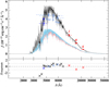 |
Fig. 4. SED of BD+20 5391. Component A is red, component B blue, and the combined model is grey. Photometric measurements are provided by Gaia/XP (black; De Angeli et al. 2023), Gaia (light blue; Riello et al. 2021), APASS (blue; Henden et al. 2016), and 2MASS (red; Skrutskie et al. 2006). Interstellar extinction was applied to the models. |
To investigate potential photometric variability due to pulsations or rotational modulation, we checked the light curve obtained from the Transiting Exoplanet Survey Satellite (TESS; Ricker et al. 2015), in particular the reduced full-frame light curves from Sector 83, available through the Barbara Mikulski Archive for Space Telescopes (MAST2). However, no significant variability was detected. Even without photometric data to constrain the rotation periods, the v sin i values of both components are similarly low and close to the spectral resolution, which suggests comparable rotation rates.
3.4. Evolution and onset of Roche lobe overflow
Leveraging the parameters derived from the SED fitting, we constrained the position of BD+20 5391 in the HRD. To further characterise the evolutionary state of both stellar components, we applied an interpolation approach based on MESA Isochrone and Stellar Tracks Collaboration (MIST; Choi et al. 2016) evolutionary tracks; this enabled a refined determination of theirproperties.
The tracks were interpolated using the scipy Python module (Virtanen et al. 2020) to create a multi-dimensional grid, enabling a smooth interpolation across initial mass, metallicity, and rotation for each equivalent evolutionary point. This interpolation function returns stellar parameters such as effective temperature (log Teff), luminosity (log L), mass, radius, and age at a given equivalent evolutionary point.
The observed stellar parameters, effective temperature and luminosity, are compared to the interpolated MIST tracks using an MCMC approach with Bayesian constraints. We then used the emcee Python module to sample the posterior distribution of the stellar parameters. In this process we minimised the likelihood function,
 (4)
(4)
where the individual chi-squared values for each star were computed based on the observed effective temperature (log Teff) and luminosity (log L) compared to the interpolated values at a given evolutionary phase, as
 (5)
(5)
To constrain the parameter space, we incorporated Gaussian prior distributions for metallicity based on the spectroscopic analysis ([Fe/H] = −0.136 ± 0.020) and for the mass ratio, as derived from the radial velocity curve (q = 0.981 ± 0.021). The resulting posterior distributions for the fitted parameters are shown in the left corner plot of Fig. A.1, and the resulting parameters are listed in Table 1.
The current semi-major axis of the binary orbit based on our fit is
 (6)
(6)
At an orbital period of only 81 days, and with a separation at periastron of  , the components of BD+20 5391 will begin mass transfer before they reach the tip of the RGB. We estimated the onset of RLOF by comparing stellar and Roche lobe radii along MIST tracks, iterating over MCMC samples to derive the corresponding age and helium core mass distribution. The Roche lobe radius was calculated using the Eggleton (1983) formula:
 (7)
(7)
where rL is the Roche lobe radius in units of separation.
The onset of RLOF was determined by comparing the stellar radius with the corresponding Roche lobe radius throughout the evolutionary track. If the stellar radius exceeds the Roche lobe radius, the star is considered to undergo RLOF. The onset of RLOF is considered to be the point where the first of the two stars fills out its Roche lobe.
At the onset of RLOF, we recorded the age, stellar radii, and helium core masses. This process was repeated for all posterior samples from the MCMC calculation, generating a distribution of RLOF ages and helium core masses. These distributions, along with the parameters derived from the fitting of the evolutionary tracks, are presented in the right plot of Fig. A.1. The corresponding values are listed in Table 1.
We performed a similar analysis using the BaSTI (Pietrinferni et al. 2021) stellar evolution models. While the resulting masses and radii are in good agreement with those previously discussed, the inferred metallicity from the HRD fit is significantly higher ([Fe/H] = +0.08) and inconsistent with the rest of our analysis. We therefore proceeded with the results based on the MIST tracks, noting that there is an intrinsic uncertainty to such model tracks.
4. Results and discussion
The MCMC techniques applied to model the evolutionary state of BD+20 5391 produced corner plots (Fig. A.1) and HRDs (Fig. 5), providing constraints on the stellar parameters. Our results indicate that RLOF is set to occur for both components before they reach the tip of the RGB. Based on our MCMC results, the two stars are expected to fill their Roche lobes at essentially the same time. The time remaining until RLOF for each component is calculated as Δτ = τRLOF − τ, yielding log ΔτA = 8.20 ± 0.04 yr and log ΔτB = 8.16 ± 0.04 yr. The delay between the two RLOF events is then given by  , which is consistent with simultaneous RLOF. Since the Eggleton formula provides an upper limit for the Roche lobe radius, the onset of mass transfer is likely to begin earlier due to additional factors such as stellar wind mass loss and the gradual expansion of the stellar atmospheres, further supporting a nearly simultaneous onset of RLOF for the two stars. This makes BD+20 5391 a strong candidate for undergoing double-core CE evolution.
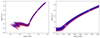 |
Fig. 5. HRD for BD+20 5391. Component A is marked in red and component B in blue. The squares denote the parameters derived from the SED and spectral fitting, while triangles indicate the onset of RLOF. The best-fit MIST evolutionary tracks are represented by discrete dots extending from the zero-age main sequence to the tip of the RGB. To visualise the uncertainties, we also show a random subset of tracks from our MCMC calculation. |
The most notable outcome of our analysis is that the helium core masses at the onset of RLOF are essentially identical: at that moment, components A and B are both predicted to have a core mass of 0.335 ± 0.003 M⊙ (statistical uncertainty only). Two primary evolutionary pathways emerge from our analysis: one in which the two stars merge and another in which they remain separate.
4.1. Merger scenario
If the binary components merge following RLOF, the combined helium core mass would be approximately 0.7 M⊙, which is sufficient for the remnant to ignite helium fusion. If the envelope is not ejected, this would result in a relatively massive red clump star. However, if the remaining envelope is expelled – which depends on the poorly constrained CE ejection efficiency – the two He cores might end up in a binary close enough that angular momentum loss through the emission of gravitational waves might lead to orbital shrinkage and an eventual merger. The remnant would likely turn into a relatively massive, core helium-burning hot subdwarf star. In particular, most helium-rich sdO (He-sdO) stars are thought to form from double He-WD mergers (Webbink 1984; Zhang & Jeffery 2012; Schwab 2018; Yu et al. 2021). Approximately one percent of He-sdOs exhibit strong magnetic fields, with average strengths between 200 and 500 kG (Dorsch et al. 2022, 2024; Pelisoli et al. 2022). Notably, all of these magnetic He-sdOs have observed masses of about 0.8 M⊙, which is close to the maximum mass attainable through He-WD mergers. This mass constraint implies that the two progenitor He-WDs must have been coeval, as expected for BD+20 5391. Indeed, Pakmor et al. (2024) recently suggested that magnetic He-sdOs originate from the merger of two equal-mass He-WDs, based on 3D magnetohydrodynamic simulations.
4.2. Non-merger scenario
If the system is able to eject a CE, but avoids merging, the result would be a double low-mass He-WD binary, likely with a short orbital period. Observational evidence of systems potentially formed through this evolutionary pathway has recently been reported by Munday et al. (2024), who identified approximately a dozen binaries with comparable component masses in the range of 0.2 to 0.4 M⊙, and by Burdge et al. (2020).
Justham et al. (2011) argue speculatively that systems consisting of two helium-rich hot subdwarfs could be the outcome of a double core CE phase as might happen for BD+20 5391. This includes the unique He-sdB binary PG 1544+4883 (Ahmad et al. 2004; Şener & Jeffery 2014).
The orbital separation after the interaction, which depends on the efficiency of mass transfer and envelope loss, will determine whether the system remains a wide double He-WD or undergoes further interactions. If the final separation is large, the system could persist as a stable double-degenerate system for a Hubble time.
5. Conclusions and outlook
Our analysis of BD+20 5391 reveals it to be a rare SB2 consisting of two nearly identical 1.4 M⊙ red giant stars in an 81-day orbit. The system’s orbital and stellar parameters suggest that the two stars have evolved in parallel without any significant mass transfer thus far.
By approximating their evolution using single-star MIST tracks, we find that the two stars will likely fill their Roche lobes almost simultaneously. This could lead to the so-called double-core evolution scenario, where the two stars orbit within a CE. Predicting their subsequent evolution requires detailed modelling that accounts for mass transfer, tidally enhanced stellar winds (Tout & Eggleton 1988; Han 1998), and the complex physics of the CE phase (Taam & Ricker 2010; Ivanova et al. 2013).
In our simplified model and given our choice of MIST tracks, both stars will have degenerate helium cores of 0.33 M⊙ when RLOF begins. If the envelope is ejected without merging, the system can evolve into a close double He-WD binary. Alternatively, the stars could merge, forming a possibly magnetic 0.7 M⊙ He-sdO, a type of star that is known to exist (Dorsch et al. 2024; Pelisoli et al. 2022; Pakmor et al. 2024).
BD+20 5391 thus provides a valuable observational benchmark for studying the progenitors of evolved compact objects such as hot subdwarfs and double He-WDs. We encourage future detailed evolutionary studies of this system. In addition, large spectroscopic surveys such as Gaia DR4+ and 4MOST (de Jong et al. 2019) will not only identify more systems like BD+20 5391 but also detect their possible descendants – double He-WDs and He-sdO stars. By observing systems before and after mass transfer, these surveys will help refine binary population synthesis models and improve our understanding oflow- and intermediate-mass binary evolution. This will build upon previous binary population synthesis studies, such as those by Han et al. (2003) for hot subdwarfs and Nelemans & Tout (2005) and van der Sluys et al. (2006) for white dwarfs.
With the release of DR3, Gaia’s Radial Velocity Spectrometer already enables the detection of some binaries and the determination of their spectroscopic orbits (Gaia Collaboration 2023b). Within the colour-magnitude selection of Uzundag et al. (2022), 19 SB2 red giants, including BD+20 5391, meet the criteria of having orbital periods between 20 and 250 days, mass ratios (q) > 0.95, and eccentricities (e) < 0.9. Future careful analyses of these systems are necessary to check whether they are genuine double RGB stars since this is not always the case: RZ Eri had previously been identified as an RGB + main sequence system (Eggleton & Yakut 2017), while BD+49 1747 and HD 7731 are likely red clump stars (Ruiz-Dern et al. 2018).
HE 0301-3039 was originally thought to be a PG 1544+488-like system (Lisker et al. 2004) but turned out to be single-lined and shows no radial velocity variations.
Acknowledgments
We thank the anonymous referee for their helpful suggestions, which have improved the quality of this paper. Research is based on data taken with the Perek telescope at the Astronomical Institute of the Czech Academy of Sciences (ASU) in Ondřejov. We thank the Stellar Physics Department of ASU and their technical staff for the support during the observations. This research was supported by funds from DAAD PPP Czech Republic project 57509654 and DAAD PPP Slovakia project 57513233. BK acknowledge the support from the Mobility Plus Project DAAD-24-02 and RVO:67985815. We thank the participants of the 2021 Ondřejov-Potsdam workshop for their observing assistance: Ayesha Arshad Arain, Saksham Arora, Radha Anil Gharapurkar, Siddarth Khalate, Chinmay Mahajan, Henrik Rose, Amrit Sedain, Tahereh Ramezani, Caiun Xia, Prapti Mondal, and Kateřina Pivoňková. MD was supported by the Deutsches Zentrum für Luft- und Raumfahrt (DLR) through grant 50-OR-2304. VS and MP were supported by the Deutsche Forschungsgemeinschaft (DFG) through grants GE2506/9-1 and GE2506/12-1, MP additionally through grant GE2506/18-1. IP acknowledges support by the DFG through grant GE2506/12-1 and from the Royal Society through a University Research Fellowship (URF/R1/231496). HD was supported by the DFG through grants GE2506/17-1 and GE2506/9-2. EK and JB acknowledge VEGA 2/0031/22. This research has used measurements obtained at the Mercator Observatory which receives funding from the Research Foundation Flanders (FWO) (grant agreement I000325N and I000521N). KD acknowledges funding from grant METH/24/012 at KU Leuven. We thank Rainer Hainich and Fabian Mattig for maintaining the Astronomical Observation Tracking System (AOTS) database. EK acknowledges support from the Slovak Research and Development Agency under contract No. APVV-20-0148. This work has made use of data from the European Space Agency (ESA) mission Gaia (https://www.cosmos.esa.int/gaia), processed by the Gaia Data Processing and Analysis Consortium (DPAC, https://www.cosmos.esa.int/web/gaia/dpac/consortium). Funding for the DPAC has been provided by national institutions, in particular the institutions participating in the Gaia Multilateral Agreement. This paper includes data collected with the TESS mission, obtained from the MAST data archive at the Space Telescope Science Institute (STScI). Funding for the TESS mission is provided by the NASA Explorer Program. STScI is operated by the Association of Universities for Research in Astronomy, Inc., under NASA contract NAS 5–26555. IRAF is distributed by the National Optical Astronomy Observatories, operated by the Association of Universities for Research in Astronomy, Inc. under a cooperative agreement with the National Science Foundation. This research has made use of NASA’s Astrophysics Data System.
References
- Ahmad, A., Jeffery, C. S., & Fullerton, A. W. 2004, A&A, 418, 275 [NASA ADS] [CrossRef] [EDP Sciences] [Google Scholar]
- Baudrand, J., & Bohm, T. 1992, A&A, 259, 711 [NASA ADS] [Google Scholar]
- Beck, P. G., Kallinger, T., Pavlovski, K., et al. 2018, A&A, 612, A22 [NASA ADS] [CrossRef] [EDP Sciences] [Google Scholar]
- Beck, P. G., Mathur, S., Hambleton, K., et al. 2022, A&A, 667, A31 [NASA ADS] [CrossRef] [EDP Sciences] [Google Scholar]
- Beck, P. G., Grossmann, D. H., Steinwender, L., et al. 2024, A&A, 682, A7 [NASA ADS] [CrossRef] [EDP Sciences] [Google Scholar]
- Belczynski, K., & Kalogera, V. 2001, ApJ, 550, L183 [CrossRef] [Google Scholar]
- Benitez-Palacios , D., Uzundag, M., Vučković, M., et al. 2025, A&A, 697, A98 [NASA ADS] [CrossRef] [EDP Sciences] [Google Scholar]
- Blanco-Cuaresma, S. 2019, MNRAS, 486, 2075 [Google Scholar]
- Brogaard, K., Arentoft, T., Slumstrup, D., et al. 2022, A&A, 668, A82 [NASA ADS] [CrossRef] [EDP Sciences] [Google Scholar]
- Brown, G. E. 1995, ApJ, 440, 270 [NASA ADS] [CrossRef] [Google Scholar]
- Burdge, K. B., Prince, T. A., Fuller, J., et al. 2020, ApJ, 905, 32 [Google Scholar]
- Cabezas, M., Šlechta, M., Škoda, P., & Kubátová, B. 2023, OESRED, the semi-automatic reduction code for Ondřejov Echelle Spectrograph [Google Scholar]
- Capitanio, L., Lallement, R., Vergely, J. L., Elyajouri, M., & Monreal-Ibero, A. 2017, A&A, 606, A65 [NASA ADS] [CrossRef] [EDP Sciences] [Google Scholar]
- Choi, J., Dotter, A., Conroy, C., et al. 2016, ApJ, 823, 102 [Google Scholar]
- Clayton, G. C. 2012, J. Am. Assoc. Variable Star Obs., 40, 539 [NASA ADS] [Google Scholar]
- Dawson, H., Geier, S., Heber, U., et al. 2024, A&A, 686, A25 [NASA ADS] [CrossRef] [EDP Sciences] [Google Scholar]
- De Angeli, F., Weiler, M., Montegriffo, P., et al. 2023, A&A, 674, A2 [NASA ADS] [CrossRef] [EDP Sciences] [Google Scholar]
- de Jong, R. S., Agertz, O., Berbel, A. A., et al. 2019, The Messenger, 175, 3 [NASA ADS] [Google Scholar]
- Dewi, J. D. M., Podsiadlowski, P., & Sena, A. 2006, MNRAS, 368, 1742 [NASA ADS] [CrossRef] [Google Scholar]
- Dorsch, M., Reindl, N., Pelisoli, I., et al. 2022, A&A, 658, L9 [NASA ADS] [CrossRef] [EDP Sciences] [Google Scholar]
- Dorsch, M., Jeffery, C. S., Philip Monai, A., et al. 2024, A&A, 691, A165 [NASA ADS] [CrossRef] [EDP Sciences] [Google Scholar]
- Duchêne, G., & Kraus, A. 2013, ARA&A, 51, 269 [Google Scholar]
- Eggleton, P. P. 1983, ApJ, 268, 368 [Google Scholar]
- Eggleton, P. P., & Yakut, K. 2017, MNRAS, 468, 3533 [NASA ADS] [CrossRef] [Google Scholar]
- El-Badry, K., Rix, H.-W., & Heintz, T. M. 2021, MNRAS, 506, 2269 [NASA ADS] [CrossRef] [Google Scholar]
- Ferrario, L., Pringle, J. E., Tout, C. A., & Wickramasinghe, D. T. 2009, MNRAS, 400, L71 [NASA ADS] [CrossRef] [Google Scholar]
- Fitzpatrick, E. L., Massa, D., Gordon, K. D., Bohlin, R., & Clayton, G. C. 2019, ApJ, 886, 108 [Google Scholar]
- Foreman-Mackey, D., Hogg, D. W., Lang, D., & Goodman, J. 2013, PASP, 125, 306 [Google Scholar]
- Gaia Collaboration (Brown, A. G. A., et al.) 2018, A&A, 616, A1 [NASA ADS] [CrossRef] [EDP Sciences] [Google Scholar]
- Gaia Collaboration (Vallenari, A., et al.) 2023a, A&A, 674, A1 [NASA ADS] [CrossRef] [EDP Sciences] [Google Scholar]
- Gaia Collaboration (Arenou, F., et al.) 2023b, A&A, 674, A34 [CrossRef] [EDP Sciences] [Google Scholar]
- Green, G. M., Schlafly, E., Zucker, C., Speagle, J. S., & Finkbeiner, D. 2019, ApJ, 887, 93 [NASA ADS] [CrossRef] [Google Scholar]
- Han, Z. 1998, MNRAS, 296, 1019 [NASA ADS] [CrossRef] [Google Scholar]
- Han, Z., Podsiadlowski, P., Maxted, P. F. L., Marsh, T. R., & Ivanova, N. 2002, MNRAS, 336, 449 [Google Scholar]
- Han, Z., Podsiadlowski, P., Maxted, P. F. L., & Marsh, T. R. 2003, MNRAS, 341, 669 [NASA ADS] [CrossRef] [Google Scholar]
- Heber, U. 2024, ArXiv e-prints [arXiv:2410.11663] [Google Scholar]
- Heber, U., Irrgang, A., & Schaffenroth, J. 2018, Open Astron., 27, 35 [Google Scholar]
- Henden, A. A., Templeton, M., Terrell, D., et al. 2016, VizieR On-line Data Catalog: II/336 [Google Scholar]
- Houck, J. C., & Denicola, L. A. 2000, ASP Conf. Ser., 216, 591 [Google Scholar]
- Iben, I., Jr, & Tutukov, A. V. 1984, ApJ, 284, 719 [NASA ADS] [CrossRef] [Google Scholar]
- Ivanova, N., Justham, S., Chen, X., et al. 2013, A&ARv, 21, 59 [Google Scholar]
- Justham, S., Podsiadlowski, P., & Han, Z. 2011, MNRAS, 410, 984 [CrossRef] [Google Scholar]
- Kabáth, P., Skarka, M., Sabotta, S., et al. 2020, PASP, 132, 035002 [CrossRef] [Google Scholar]
- Koubský, P., Mayer, P., Čáp, J., et al. 2004, Publ. Astron. Inst. Czechoslovak Acad. Sci., 92, 37 [Google Scholar]
- Kounkel, M., Covey, K. R., Stassun, K. G., et al. 2021, AJ, 162, 184 [NASA ADS] [CrossRef] [Google Scholar]
- Kurucz, R. L. 1993, SYNTHE spectrum synthesis programs and line data [Google Scholar]
- Kurucz, R. 2013, Astrophysics Source Code Library 03024 [Google Scholar]
- Li, Z., Chen, X., Chen, H.-L., & Han, Z. 2019, ApJ, 871, 148 [NASA ADS] [CrossRef] [Google Scholar]
- Lindegren, L., Bastian, U., Biermann, M., et al. 2021, A&A, 649, A4 [EDP Sciences] [Google Scholar]
- Lisker, T., Heber, U., Napiwotzki, R., et al. 2004, Ap&SS, 291, 351 [NASA ADS] [CrossRef] [Google Scholar]
- Munday, J., Pelisoli, I., Tremblay, P. E., et al. 2024, MNRAS, 532, 2534 [NASA ADS] [CrossRef] [Google Scholar]
- Nelemans, G., & Tout, C. A. 2005, MNRAS, 356, 753 [NASA ADS] [CrossRef] [Google Scholar]
- Offner, S. S. R., Moe, M., Kratter, K. M., et al. 2023, ASP Conf. Ser., 534, 275 [NASA ADS] [Google Scholar]
- Paczynski, B. 1976, IAU Symp., 73, 75 [NASA ADS] [Google Scholar]
- Pakmor, R., Pelisoli, I., Justham, S., et al. 2024, A&A, 691, A179 [NASA ADS] [CrossRef] [EDP Sciences] [Google Scholar]
- Pelisoli, I., Dorsch, M., Heber, U., et al. 2022, MNRAS, 515, 2496 [NASA ADS] [CrossRef] [Google Scholar]
- Pietrinferni, A., Hidalgo, S., Cassisi, S., et al. 2021, ApJ, 908, 102 [NASA ADS] [CrossRef] [Google Scholar]
- Pribulla, T., Garai, Z., Hambálek, L., et al. 2015, Astron. Nachr., 336, 682 [NASA ADS] [CrossRef] [Google Scholar]
- Raskin, G. 2011, Ph.D. Thesis, Katholieke University of Leuven Astronomical Institute [Google Scholar]
- Rawls, M. L., Gaulme, P., McKeever, J., et al. 2016, ApJ, 818, 108 [Google Scholar]
- Ricker, G. R., Winn, J. N., Vanderspek, R., et al. 2015, J. Astron. Telescopes Instrum. Syst., 1, 014003 [Google Scholar]
- Riello, M., De Angeli, F., Evans, D. W., et al. 2021, A&A, 649, A3 [NASA ADS] [CrossRef] [EDP Sciences] [Google Scholar]
- Ruiz-Dern, L., Babusiaux, C., Arenou, F., Turon, C., & Lallement, R. 2018, A&A, 609, A116 [NASA ADS] [CrossRef] [EDP Sciences] [Google Scholar]
- Schlafly, E. F., & Finkbeiner, D. P. 2011, ApJ, 737, 103 [Google Scholar]
- Schlegel, D. J., Finkbeiner, D. P., & Davis, M. 1998, ApJ, 500, 525 [Google Scholar]
- Schwab, J. 2018, MNRAS, 476, 5303 [Google Scholar]
- Åžener, H. T., & Jeffery, C. S. 2014, MNRAS, 440, 2676 [NASA ADS] [CrossRef] [Google Scholar]
- Shao, Y., & Li, X.-D. 2014, ApJ, 796, 37 [Google Scholar]
- Skrutskie, M. F., Cutri, R. M., Stiening, R., et al. 2006, AJ, 131, 1163 [NASA ADS] [CrossRef] [Google Scholar]
- Taam, R. E., & Ricker, P. M. 2010, New Astron. Rev., 54, 65 [CrossRef] [Google Scholar]
- Tody, D. 1986, SPIE Conf. Ser., 627, 733 [Google Scholar]
- Tody, D. 1993, The IRAF mail network, 26, 791 [Google Scholar]
- Tout, C. A., & Eggleton, P. P. 1988, MNRAS, 231, 823 [NASA ADS] [CrossRef] [Google Scholar]
- Traven, G., Feltzing, S., Merle, T., et al. 2020, A&A, 638, A145 [NASA ADS] [CrossRef] [EDP Sciences] [Google Scholar]
- Tutukov, A. V., & Fedorova, A. V. 2010, Astron. Rep., 54, 156 [CrossRef] [Google Scholar]
- Uzundag, M., Jones, M. I., Vučković, M., et al. 2022, A&A, 668, A89 [NASA ADS] [CrossRef] [EDP Sciences] [Google Scholar]
- van der Sluys, M. V., Verbunt, F., & Pols, O. R. 2006, A&A, 460, 209 [NASA ADS] [CrossRef] [EDP Sciences] [Google Scholar]
- Virtanen, P., Gommers, R., Oliphant, T. E., et al. 2020, Nat. Methods, 17, 261 [Google Scholar]
- Webbink, R. F. 1984, ApJ, 277, 355 [NASA ADS] [CrossRef] [Google Scholar]
- Yu, J., Zhang, X., & Lü, G. 2021, MNRAS, 504, 2670 [NASA ADS] [CrossRef] [Google Scholar]
- Zhang, X., & Jeffery, C. S. 2012, MNRAS, 419, 452 [NASA ADS] [CrossRef] [Google Scholar]
Appendix A: Additional material
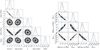 |
Fig. A.1. Corner plots displaying the posterior distributions of key parameters derived from the MCMC analysis. Left: Parameter distributions from the best-fit evolutionary model. Right: Posterior distributions at the point of RLOF. |
Heliocentrically corrected radial velocity (RV) measurements.
All Tables
All Figures
|
Fig. 1. Colour-magnitude diagram of observed red giant stars, based on Gaia DR3 (Gaia Collaboration 2023a). The sample includes RGB stars just below the red clump within 500 pc of the Sun. Blue triangles mark spectra from OES, red circles from AISAS. BD+20 5391 is highlighted in yellow. The grey background marks all Gaia DR3 objects with parallax_over_error > 100 within 500 pc of the Sun. |
| In the text | |
|
Fig. 2. Radial velocity curve of BD+20 5391 for components A (red) and B (blue). Circles show measurements obtained with the OES, and the triangles mark the HERMES measurement. |
| In the text | |
|
Fig. 3. Selected ranges in the double-lined HERMES spectrum of BD+20 5391. The upper section shows the observed data in light grey and the combined model fit as a dashed black line, while the lower part displays the contributions of the individual components, offset by −0.5 for clarity. Component A is shown in red, component B in blue; strong lines are labelled. |
| In the text | |
|
Fig. 4. SED of BD+20 5391. Component A is red, component B blue, and the combined model is grey. Photometric measurements are provided by Gaia/XP (black; De Angeli et al. 2023), Gaia (light blue; Riello et al. 2021), APASS (blue; Henden et al. 2016), and 2MASS (red; Skrutskie et al. 2006). Interstellar extinction was applied to the models. |
| In the text | |
|
Fig. 5. HRD for BD+20 5391. Component A is marked in red and component B in blue. The squares denote the parameters derived from the SED and spectral fitting, while triangles indicate the onset of RLOF. The best-fit MIST evolutionary tracks are represented by discrete dots extending from the zero-age main sequence to the tip of the RGB. To visualise the uncertainties, we also show a random subset of tracks from our MCMC calculation. |
| In the text | |
|
Fig. A.1. Corner plots displaying the posterior distributions of key parameters derived from the MCMC analysis. Left: Parameter distributions from the best-fit evolutionary model. Right: Posterior distributions at the point of RLOF. |
| In the text | |
Current usage metrics show cumulative count of Article Views (full-text article views including HTML views, PDF and ePub downloads, according to the available data) and Abstracts Views on Vision4Press platform.
Data correspond to usage on the plateform after 2015. The current usage metrics is available 48-96 hours after online publication and is updated daily on week days.
Initial download of the metrics may take a while.