| Issue |
A&A
Volume 702, October 2025
|
|
|---|---|---|
| Article Number | A9 | |
| Number of page(s) | 11 | |
| Section | Stellar structure and evolution | |
| DOI | https://doi.org/10.1051/0004-6361/202556234 | |
| Published online | 26 September 2025 | |
New line-driven wind mass-loss rates for OB stars with metallicities down to 0.01 Z⊙
1
Department of Theoretical Physics and Astrophysics, Faculty of Science, Masaryk University, CZ-611 37 Brno, Czech Republic
2
Astronomical Institute, Czech Academy of Sciences, CZ-251 65 Ondřejov, Czech Republic
⋆ Corresponding author.
Received:
3
July
2025
Accepted:
27
July
2025
Abstract
We provide new line-driven wind models for OB stars with metallicities down to 0.01 Z⊙. The models were calculated with our global wind code METUJE, which solves the hydrodynamical equations from nearly hydrostatic photosphere to supersonically expanding stellar wind together with the equations of statistical equilibrium and the radiative transfer equation. The models predict the basic wind parameters, namely, the wind mass-loss rates and terminal velocities just from the stellar parameters. In general, the wind mass-loss rates decrease with decreasing metallicity and this relationship steepens for very low metallicities, Z ≲ 0.1 Z⊙. Down to metallicities corresponding to the Magellanic Clouds and even lower, the predicted mass-loss rates reasonably agree with observational estimates. However, the theoretical and observational mass-loss rates for very low metallicities exhibit significant scatter. We show that the scatter of observational values can be caused by inefficient shock cooling in the stellar wind, which leaves a considerable fraction of the wind at too high temperatures with waning observational signatures. The scatter of theoretical predictions is caused by a low number of lines that effectively accelerate the wind at very low metallicities.
Key words: stars: early-type / stars: mass-loss / supergiants / stars: winds / outflows / Local Group / Magellanic Clouds
© The Authors 2025
 Open Access article, published by EDP Sciences, under the terms of the Creative Commons Attribution License (https://creativecommons.org/licenses/by/4.0), which permits unrestricted use, distribution, and reproduction in any medium, provided the original work is properly cited.
This article is published in open access under the Subscribe to Open model. This email address is being protected from spambots. You need JavaScript enabled to view it. to support open access publication.
1. Introduction
On the way from their formation toward their final core collapse, massive stars tend to lose most of their initial mass. The process of mass loss significantly influences the evolutionary pathways of these stars (Renzo et al. 2017; Keszthelyi et al. 2017). A considerable fraction of the stellar mass is lost via line-driven winds. These are long-lasting outflows, which are accelerated mostly by the momentum acquired from the radiation field via line absorption (Vink 2022, for a review). However, the implications of winds go far beyond their impact on the stellar evolution. Winds shape the interaction regions between massive stars and circumstellar environment (Gvaramadze et al. 2018; Kobulnicky et al. 2019), where the high-energy particles can be accelerated (Bednarek 2024; Peron et al. 2024), and contribute to the enrichment of the interstellar medium with heavy elements (Szécsi & Wünsch 2019).
Because the stellar winds of hot stars are driven mostly by line transitions of heavy elements, the strength of the wind depends on the abundance of each element. The dependence on metallicity is usually parameterized via the total mass fraction of heavier elements, Z, which is often a reasonable proxy. For instance, in O stars at metallicities higher than about 0.1 Z⊙, the rotational mixing, which brings freshly synthesized nitrogen at the expense of carbon and oxygen to the stellar surface, does not significantly affect basic wind properties (Krtička & Kubát 2014).
The mass-loss rate, Ṁ, is the key wind parameter, which gives the amount of mass lost by the star per unit of time. The metallicity dependence of the wind mass-loss rate is typically parameterized via power law, namely, Ṁ ∼ Zα. As follows from theoretical calculations (Puls et al. 2000), the power-law index, α, is related to the line-strength distribution parameters  and
and  as
as  . For a canonical value
  with
with  this gives a square-root dependence of mass-loss rate on metallicity α = 0.5. Calculations based on the Sobolev approximation with a realistic line-list give α = 0.94 (Abbott 1982), which is not too far but somewhat higher than the value derived from Monte Carlo calculations of α = 0.69 (Vink et al. 2001). Models based on the comoving-frame radiative transfer calculations (Krtička & Kubát 2018) give even lower value of α = 0.59, which is close to the canonical value mentioned above (α = 0.5). Their mass-loss rate scaling with metallicity also agrees with empirical estimates (Marcolino et al. 2022).
The terminal velocity, v∞, is another important wind parameter, which gives the speed of the wind at large distances from the star. Unlike the mass-loss rate, the wind terminal velocity only weakly depends on the metallicity and is mostly given by the escape speed from the stellar surface multiplied by the factor  (Castor et al. 1975). Therefore, the metallicity dependence of the terminal velocity stems from the variations of the
  parameter with metallicity. Detailed calculations do not offer any clear predictions concerning the dependence of wind terminal velocity on the metallicity (Krtička et al. 2024), partly because the terminal velocity is given by the integration of equation of motion over large interval of radii. Therefore, wind terminal velocity might be strongly affected by uncertainties of the radiative force connected, for example, with the influence of X-rays or clumping (e.g., Carneiro et al. 2016; Krtička et al. 2018; Sander & Vink 2020).
The observational analysis shows that the wind terminal velocity is correlated not only with the escape speed, but also with the stellar effective temperature (Prinja et al. 1990; Hawcroft et al. 2024b). Moreover, the observations indicate slight increase in the wind terminal velocity with metallicity, v∞ ∼ Z0.22 (Hawcroft et al. 2024b). While the variation in the terminal speed with effective temperature can be understood as coming from evolutionary effects (Kudritzki & Puls 2000; Krtička et al. 2024), the theoretical predictions of the wind terminal velocity variations with metallicity are ambiguous. Krtička & Kubát (2018) did not predict any strong correlation between the wind terminal velocity and metallicity; whereas Sander & Vink (2020) showed an increase in the wind terminal velocity with metallicity for optically thick winds of helium stars and the calculations from Björklund et al. (2021) offered predictions of different slopes for the variations in the dependence on luminosity. In any case, any variations of the wind terminal velocity with metallicity are likely weak, as exemplified in the case of stars from IC 1613, which are expected to have even lower metallicity than stars from the Large and Small Magellanic Clouds (LMC and SMC), while still exhibiting similar terminal velocities (Garcia et al. 2014).
Theoretical wind parameter estimates are typically confined to metallicities corresponding to our Galaxy and the LMC and SMC (e.g., Gormaz-Matamala et al. 2022; Björklund et al. 2023; Krtička et al. 2024) corresponding to the range of metallicities of 0.2 ≤ Z/Z⊙ ≤ 1. This metallicity range is well covered also by observational surveys, such as ULLYSES (Roman-Duval et al. 2025) and XShootU (Vink et al. 2023). However, observational studies become possible also for stars at even lower metallicities (Garcia et al. 2014; Telford et al. 2024). The theoretical wind predictions for stars at even lower metallicities than that corresponding to the SMC are scarce. Therefore, to enable test of the wind models for even lower metallicities, we provide mass-loss rate predictions for OB stars with metallicities down to 0.01Z/Z⊙ based on our METUJE code.
2. Wind models
State-of-the-art mass-loss rate predictions in hot stars are based on global (unified) wind models (Gräfener & Hamann 2008; Krtička & Kubát 2017; Sundqvist et al. 2019), which solve the radiative transfer equation line by line from IR to UV regions and self-consistently account for the interaction between the stellar wind and photosphere. In particular, we applied our METUJE global wind code (Krtička & Kubát 2017), which solves wind equations from nearly hydrostatic photosphere to supersonically expanding wind, while assuming spherical symmetry and stationarity.
The METUJE code determines radial variations of wind density, radial velocity, and temperature by solving corresponding hydrodynamical equations together with the radiative transfer and kinetic (statistical) equilibrium equations (usually referred to as the NLTE modeling). This allows us to consistently predict wind mass-loss rate from the equation of continuity and wind terminal speed from the equation of motion. The radiative force and radiative heating and cooling terms are derived from the solution of the radiative transfer equation, which is solved frequency by frequency in the comoving frame (Mihalas et al. 1975). The calculated radiation field is further used to determine the influence of the radiation processes on the level populations via kinetic equilibrium equations (Hubeny & Mihalas 2014). These equations are solved for most abundant elements (listed in Krtička et al. 2020), which can significantly contribute either to the radiative driving or heating. The models are calculated assuming a smooth wind neglecting small-scale structure (clumping).
METUJE solves all equations iteratively allowing us to determine a consistent solution of wind equations. The initial estimate of atmospheric structure is derived from TLUSTY stellar atmosphere code (Lanz & Hubeny 2003, 2007). We typically calculate the TLUSTY models for the same parameters as METUJE models; however, for subMagellanic metallicities, using models with SMC composition was sufficient in most cases.
In this work, the models were parameterized by the stellar effective temperature, Teff, stellar mass, M, radius, R*, and surface chemical composition. The resulting grid of wind parameters covers O main-sequence stars, giants, and supergiants and B supergiants. For O stars, we selected the same grid of stellar parameters as in Krtička & Kubát (2018), which was derived using relations of Martins et al. (2005). The grid for B supergiants was calculated at three different values of stellar luminosity, L, for the same stellar parameters as in Krtička et al. (2021). The selected parameters correspond to typical values determined for B supergiants from our Galaxy (Crowther et al. 2006). The models were calculated for three different metallicities Z⊙/10, Z⊙/30, and Z⊙/100 derived by scaling solar chemical composition (Z⊙) of Asplund et al. (2009) for each individual element.
3. Calculated wind parameters
Predicted values of wind mass-loss rates and terminal velocities are given in Table 1 for B supergiants and in Table 2 for O stars. For the subsequent analysis, these models were complemented with OB star wind models at Galactic (Z⊙), LMC (Z⊙/2), and SMC (Z⊙/5) metallicities calculated earlier with the same code for the same stellar masses, luminosities, and radii (Krtička & Kubát 2017, 2018; Krtička et al. 2021, 2024).
Predicted terminal velocities v∞ (in km s−1) and the mass-loss rates Ṁ (in M⊙ yr−1) for B supergiants.
Predicted terminal velocities v∞ (in km s−1) and the mass-loss rates Ṁ (in M⊙ yr−1) for O stars.
In general, the mass-loss rate increases with increasing luminosity and metallicity; in addition, it depends on the effective temperature. With increasing luminosity, the radiative force and, consequently, mass-loss rate also increase (Fig. 1).
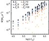 |
Fig. 1. Wind mass-loss rate as a function of the stellar luminosity from METUJE models at different metallicities for stars with Teff ≥ 27.5 kK. |
The metallicity dependence of the wind mass-loss rate stems from increase in the line opacity with increasing metallicity, which increases the line radiative force. The decrease in the wind mass-loss rate with decreasing metallicity is already visible from the downward shift of luminosity variations plotted for different metallicities in Fig. 1. Moreover, this plot also shows that while the luminosity dependence of the mass-loss rate is monotonic for higher metallicities, for subMagellanic metallicities (Z ≲ 0.1 Z⊙), the luminosity relationship shows scatter, which is a particularly considerable one for Z = 0.01 Z⊙. The metallicity dependence of the mass-loss rate is further demonstrated in Fig. 2, where we plot the steepness of the metallicity dependence of the mass-loss rate, Ṁ ∼ Zα,
 (1)
(1)
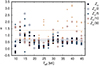 |
Fig. 2. Power of the metallicity dependence of the mass-loss rate Ṁ ∼ Zα (Eq. (1)) plotted as a function of the stellar effective temperature for models at different metallicities. Dashed lines describe mean relationship derived for individual metallicities. |
as a function of the effective temperature. The parameter α is evaluated for stellar models in Tables 1 and 2. The plot in Fig. 2 approximates the derivative using backward differences calculated for metallicities from the grid. For example, the α value at the solar metallicity is approximated as  . Consequently, there is no value for α(0.01 Z⊙). From the plot, it follows that while at the metallicities corresponding to our Galaxy and the Magellanic Clouds the metallicity dependence of the mass-loss rate can be approximated by a single relationship Ṁ ∼ z0.60, for lower metallicities (Z ≲ 0.1 Z⊙) the relationship significantly steepens, even reaching as high as Ṁ ∼ Z1.4 for Z⊙/30.
The variations in the power α with the temperature are not monotonic, but they do show a maximum around Teff ≈ 15 kK and a significant scatter for subMagellanic metallicities (Z ≲ 0.1 Z⊙) in Fig. 2. These variations can be understood using Fig. 3, where we plot contribution of individual elements to the radiative force. The radiative driving in the O star domain is dominated by CNO elements, while iron dominates in B supergiants at solar metallicity (Vink et al. 1999), which is replaced by silicon at subMagellanic abundances. These variations stem from dependence of flux distribution and ionization degree on the effective temperature. In the O star domain, a significant fraction of line driving originates in the spectral region of the Lyman continuum (Abbott 1982), where ions such as N IV, O V, and Ne IV have many strong lines driving the wind. As the temperature decreases, the maximum of the flux distribution shifts to the Balmer continuum, and ionization balance of CNO elements becomes dominated by C III, N III, and O II. However, these ions also have the strongest resonance lines in the Lyman continuum and this mismatch between the wavelength of the maximum flux and the position of the strongest lines leads to a decrease in the contribution of CNO elements to the radiative force1. Instead, a significant contribution of Fe III appears at solar metallicity, which has a large number of strong lines at longer wavelengths. However, the iron lines become optically thin at subMagellanic metallicities and iron contribution is replaced by Si IV, whose 1394 Å and 1403 Å resonance doublet together with C III 977 Å line might provide more than two thirds of the line acceleration at the lowest metallicities in the region of the critical point.
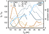 |
Fig. 3. Relative contribution of selected elements to the line radiative force as a function of the effective temperature, plotted at the wind critical point for O giants and B supergiants with M = 40 M⊙. While line colors denote individual elements, line styles differentiate between metallicity, with the solid line corresponding to Z⊙, dashed line to 0.1 Z⊙, and dotted line to 0.01 Z⊙. The thick blue line gives the mean ionization state driving the wind for 0.1 Z⊙. The mean ionization state is defined as ∑fizi/(∑fi), where fi is the contribution of ion i (with charge zi) to the line radiative force. The corresponding axis is on the right. The values of the radiative force were obtained within the Sobolev approximation. |
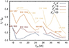 |
Fig. 4. Relative contribution of three lines that drive the wind most strongly to the radiative force. Plotted as a function of the stellar effective temperature for different metallicities at the critical point using the Sobolev approximation for O giants and 40 M⊙ B supergiants. We labeled selected strongest lines with wavelength in Å. |
The contribution of individual lines to the radiative force is further illustrated in Fig. 4, which gives the cumulative fraction of the radiative force coming from the three strongest lines. For higher metallicities, the contribution of the three strongest lines to the radiative force is typically below 10%. This implies that the wind is driven by a large number of lines at high metallicities. However, with decreasing metallicity, many of the strong lines become optically thin and their contribution to the radiative force becomes quenched. As a result, the wind is driven just by a few lines at the lowest metallicities.
The low number of lines that significantly drive the wind at the lowest metallicities leads to a strong variation in the mass-loss rate with stellar parameters. This can be seen as a high dispersion in the plots of the dependence of the mass-loss rate on luminosity in Fig. 1 and the power of metallicity dependence (Fig. 2) for Z ≤ 0.1 Z⊙. The decrease in the mass-loss rate with metallicity is not only caused directly by a decreased metallicity, but also indirectly by a reduced wind density. Lower wind density leads to ionization shift toward higher ions, which drive the wind less efficiently, leading to decrease in the mass-loss rate. For instance, the wind of a 400-1 star is driven to a large fraction by such ions as O IV and Ne IV. With decreasing metallicity, the line force decreases, leading to the reduction of the wind density. The decrease in the density leads to higher ionization, diminishes the ionization fraction of O IV and Ne IV and further reduces the mass-loss rate. As a result, the metallicity power α becomes very high around Teff ≈ 40 kK. Below and above this temperature, the changes due to ionization are not so high; therefore, α is lower.
A high value of the metallicity power α at Teff ≈ 15 kK in Fig. 2 is caused by yet another effect. Our models feature so-called bistability bump at solar metallicity in this temperature domain (Pauldrach & Puls 1990), which is caused by increase in the line force due to iron recombination from Fe IV to Fe III (Vink et al. 1999; Vink 2018; Krtička et al. 2021). With decreasing metallicity, the iron lines become optically thin, theircontribution to the radiative force decreases (Fig. 3) and the bistability jump vanishes. As a result, α is higher than one for Z ≳ 0.2 Z⊙ around Teff ≈ 15 kK.
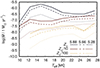 |
Fig. 5. Mass-loss rate variations with the temperature for B supergiants. The line color denotes metallicity, while the dash type corresponds to different stellar luminosities (log(L/L⊙) = 5.28, 5.66, and 5.88). |
The metallicity variations of the bistability jump are apparent also in Fig. 5 showing the mass-loss rate as a function of the effective temperature for different stellar luminosities. At solar metallicity, a clear maximum appears at about 15 kK, which weakens for lower metallicities and shifts toward lower temperatures (Vink et al. 2001, as follows from their Eqs. (14) and (15)). The shift appears due a stronger ionization in winds with lower densities. The extended width of the bistability region results from gradual dependence of recombination of Fe IV on temperature. The latter ion dominates at high effective temperatures, but at 20 kK the first part of the wind dominated by Fe III appears. Fe III starts to dominate the whole wind at Teff ≈ 15 kK or even cooler at low metallicities. Petrov et al. (2016) found a narrow bistability jump and at a higher effective temperature of 21 kK. This is likely the result of their adopted terminal velocity variation, which is based on the empirical results of Lamers et al. (1995), featuring a jump. Crowther et al. (2006) found smooth variations of the ratio of the wind terminal velocities and the escape speed, which likely smooths the jump in mass-loss rates. Vink (2018) also found smooth bistability jump and increasing wind mass-loss rate even below 20 kK from the consistent solution of the momentum equation. Calculations of Björklund et al. (2023) do not predict any bistability jump from their models. The reason for this absence is not fullyclear.
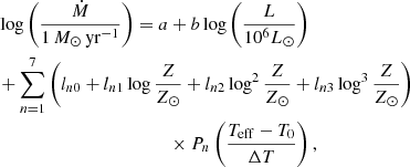
As a result of strong variations of the mass-loss rate with stellar parameters (mainly temperature), we were unable to derive a precise fit of the predicted mass-loss rates. Nonetheless, the mass-loss rates can be roughly fitted via a rather sloppyfit as
![Mathematical equation: $$ \begin{aligned} \log \left(\frac{\dot{M}}{1\, {M}_{\odot }\,\mathrm{yr}^{-1}} \right)&= \tilde{a} +\tilde{b} \log \left(\frac{L}{10^6L_\odot }\right) +\tilde{c}\log \left(\frac{Z}{Z_\odot }\right)+ \tilde{d}\log \left(\frac{T_{\rm eff}}{10^3\,\mathrm{K}}\right)\nonumber \\&\qquad + \tilde{e}\left(\frac{Z}{Z_\odot }\right) \exp \left[-\frac{(T_{\rm eff}-\tilde{T}_0)^2}{\Delta \tilde{T}^2}\right]. \end{aligned} $$](/articles/aa/full_html/2025/10/aa56234-25/aa56234-25-eq17.gif) (2)
(2)
Throughout our paper, log denotes decadic logarithm and exp the natural exponential function. Parameters of the fit are given in Table 3. The fit does not represent the predicted mass-loss rates particularly well with root mean square (rms) of the residual of about 0.28 dex and a maximum deviation for individual stars as high as a factor of 3.
A fussier fit can be derived using Legendre polynomials2
 (3)
(3)
where Pn(x) are Legendre polynomials of a degree, n, 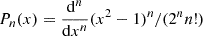 . The individual parameters are given in Table 4. This this fit does not represent the predicted mass-loss rates very well, with a rms of the residual of about 0.17 dex, while the deviations for some stars could be as high as a factor of 2. The differences between the mass-loss rates derived from the models and from the fit Eq. (3) increase toward lower metallicities. The fits in Eqs. (2) and (3) were derived for abundances of Z = 0.01 − 1 Z⊙ and effective temperatures of 10 − 45 kK; thus, their usage outside this range of parameters can lead to erroneous results.
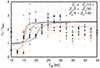 |
Fig. 6. Predicted ratio of the wind terminal velocity, v∞, and escape speed, vesc, as a function of the effective temperature. Solid lines colored according to the metallicity give fit to theoretical predictions (see Eq. (4)). |
The wind terminal velocity depends mostly on the escape speed and on stellar parameters such as stellar temperature and metallicity (Castor et al. 1975; Puls et al. 2000). Figure 6 demonstrates that this relationship is not smooth, but shows a considerable scatter. On average, the terminal velocity is nearly independent on metallicity for OB stars above the bistability jump (Teff ≥ 20 kK) with Z ≥ 0.2 Z⊙, while it scales roughly as v∞ ∼ Z0.18 for lower metallicities. On average, the ratio of the terminal velocity to the escape speed can be approximated as
![Mathematical equation: $$ \begin{aligned} \frac{v_\infty }{v_{\rm esc}}&= \frac{1}{2}\left[\left(v_+-v_-\right)\frac{t}{1+|t|}+v_++v_-\right],\end{aligned} $$](/articles/aa/full_html/2025/10/aa56234-25/aa56234-25-eq20.gif) (4)
(4)
 (5)
(5)
 (6)
(6)
where the fit parameters are given in Table 5. The fit was derived for stars with Teff ≤ 30 kK. Regarding the upper limit, the wind terminal velocity of stars with Teff ≥ 30 kK becomes affected by clumping (Krtička et al. 2018); consequently, we disregarded this region for the fit.
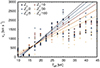 |
Fig. 7. Predicted wind terminal velocity as a function of the effective temperature for different metallicities. The linear fits are colored according to metallicity and derived from Eq. (7). |
From the observational analysis, it follows that the wind terminal velocity scales with the effective temperature (Prinja et al. 1990; Hawcroft et al. 2024b). We plot this relation derived from our models in Fig. 7. The theoretical predictions can be fitted as
![Mathematical equation: $$ \begin{aligned} \left(\frac{v_\infty }{\mathrm{km\,s}^{-1}}\right) = \left[v_a+v_{az}\log \left(\frac{Z}{Z_\odot }\right)\right] \left(\frac{T_{\rm eff}}{10^3\,\mathrm{K}}\right)+v_b+v_{bz}\log \frac{Z}{Z_\odot }. \end{aligned} $$](/articles/aa/full_html/2025/10/aa56234-25/aa56234-25-eq23.gif) (7)
(7)
The parameters of the fit are given in Table 6. These parameters were derived for 12.5 kK ≤ Teff ≤ 30 kK.
4. Comparison with observational estimates
There are several diagnostics that can be used to determine the wind mass-loss rates from observations, including near-infrared (NIR) line spectroscopy (Najarro et al. 2011), optical, and ultraviolet (UV) spectroscopy (Bouret et al. 2012; Šurlan et al. 2013), X-ray line profiles (Cohen et al. 2014), and wind bow shocks (Kobulnicky et al. 2019). However, at low metallicities, only results based on optical and UV analysis are typically available. To obtain a homogeneous observational sample, we focus only on the mass-loss rates estimated from optical and UV line spectroscopy that accounts for wind clumping. These values were obtained typically within the ULLYSES (Roman-Duval et al. 2025) and XShootU (Vink et al. 2023) projects in the case of the LMC and SMC.
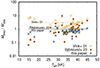 |
Fig. 8. Ratio of the predicted mass-loss rates and their observational estimates plotted as a function of the stellar effective temperature for stars from our Galaxy. The theoretical mass-loss rates from Vink et al. (2001), Björklund et al. (2023), and this paper are compared with observational estimates of Najarro et al. (2011), Bouret et al. (2012), Šurlan et al. (2013), Marcolino et al. (2017, supergiants), Hawcroft et al. (2021), and Bernini-Peron et al. (2023). The horizontal lines give mean values for individual theoretical predictions. |
Figure 8 compares the observational estimates with theoretical predictions calculated for parameters of individual stars from Galaxy. On average, the mean ratio of the theoretical values and observational determination is 0.94, which just slightly underestimates the observations, but the median is about 0.7. The predictions of Björklund et al. (2023) give comparable ratio of 1.13, but the mass-loss rates are underestimated by a factor of about 10 in the B star domain (Bernini-Peron et al. 2023). The predictions of Vink et al. (2001) overestimate the mass-loss rates on average by a factor of about 2.9. The ratio of the theoretical to observational estimates is nearly the same reported in the observational analysis of Bouret et al. (2012), which assumes optically thin clumps, as well as in Šurlan et al. (2013) and Hawcroft et al. (2021), where optically thick clumps were allowed. This indicates that the current approach to modeling of optically thick clumps does not introduce a systematic shift in estimated mass-loss rates (Hawcroft et al. 2021; Brands et al. 2025).
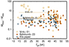 |
Fig. 9. Ratio of the predicted mass-loss rates and their observational estimates plotted as a function of the effective temperature for stars from the LMC. The theoretical mass-loss rates from Vink et al. (2001), Björklund et al. (2023), and this paper are compared with observational estimates of Brands et al. (2022), Hawcroft et al. (2024a), and Verhamme et al. (2024). The horizontal lines give mean values for individual theoretical predictions. |
Figure 9 gives a similar plot for the LMC. The mean ratio of the theoretical and observational mass-loss rates is 1.3 (for stars with Teff < 47 kK). The ratio is about 1.6 for mass-loss rates of Björklund et al. (2023) and about 7 for mass-loss rates of Vink et al. (2001).
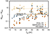 |
Fig. 10. Ratio of the predicted mass-loss rates and their observational estimates plotted as a function of the effective temperature for stars from the SMC. The theoretical mass-loss rates from Vink et al. (2001), Björklund et al. (2023), and this paper are compared with observational estimates of Bouret et al. (2013, 2021), Backs et al. (2024), and Bernini-Peron et al. (2024). The horizontal lines give mean values for individual theoretical predictions. |
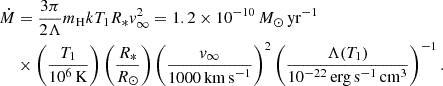
For the SMC our mass-loss rates overestimate the observational results by a factor of 2.8, while the rates of Björklund et al. (2023) perform better and give a mean ratio of about 1.2. However, these rates underestimate the mass-loss rates of B supergiants by an order of magnitude (see Bernini-Peron et al. 2024), while our mass-loss rates offer a reasonable fit. The rates of Vink et al. (2001) overestimate the observational values by a factor of about 7. Moreover, winds of stars with low mass-loss rates may be affected by weak-wind problem (Sect. 5.3). By disregarding stars with observational mass-loss rates lower than 3 × 10⁻⁸ M⊙ yr−1, we obtain a much more favorable ratio of the theoretical and observational mass-loss rates of about 1.0 (Fig. 10). On this basis, we can conclude that the poor agreement between our predictions and observational estimates for the SMC only applies to stars with a very low mass-loss rate and is likely caused by the inefficient shock cooling (Sect. 5.3).
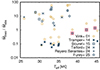 |
Fig. 11. Ratio of the predicted mass-loss rates and their observational estimates plotted as a function of the effective temperature for stars from galaxies with subMagellanic metallicities. Pink box denotes the only three stars with clumping-corrected mass-loss rate Ṁ > 10−7 M⊙ yr−1. |
These results are summarized in Table 7, which gives mean ratio of theoretical mass-loss rate predictions and observational determinations  . In addition, it includes the rms of residuals of this ratio,
 (8)
(8)
Mass-loss rate estimates for galaxies with metallicities lower than corresponding to the SMC are rare. Tramper et al. (2014) derived mass-loss rates of nine O-type stars in low-metallicity galaxies IC 1613, WLM, and NGC 3109 from optical spectroscopy neglecting clumping. Three of these stars were subsequently reanalyzed by Bouret et al. (2015) using UV spectroscopy. Telford et al. (2024) estimated mass-loss rates in three O stars in the nearby dwarf galaxies Leo P, Sextans A, and WLM, with abundances of 0.03 − 0.14 Z⊙. Reyero Serantes et al. (2024) derived the mass-loss rate estimate of the X-1 donor star in Holmberg II dwarf galaxy with a metallicity of 0.07 Z⊙ (Kaaret et al. 2004). Furey et al. (2025) derived wind properties of massive stars from five galaxies with subMagellanic metallicities down to Z = 0.03 Z⊙. All these predictions are plotted in Fig. 11 in comparison to the theoretical estimates. Apparently, the figure shows a relatively large scatter. As a result of weakness of these winds, a part of this scatter is caused by the weak-wind problem (Sect. 5.3). On the other hand, the prediction for the only three stars with the mass-loss rate higher than 10−7 M⊙ yr−1 and determined accounting for clumping (pink squares in Fig. 11) agree well with observations.
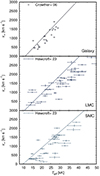 |
Fig. 12. Observational values of the wind terminal velocities (Crowther et al. 2006; Hawcroft et al. 2024b) compared with theoretical predictions Eq. (7) for stars from the Galaxy, LMC, and SMC. |
The linear fit of wind terminal velocities Eq. (7) obtained for stars with Teff ≤ 30 kK reasonably agrees with observational determinations not only in the domain of B supergiants, but also for luminous O stars (Fig. 12). A similar comparison for galaxies with subMagellanic metallicities shows lower than predicted terminal velocities in some stars (Fig. 13). Overall, however, the agreement is reasonable.
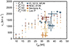 |
Fig. 13. Observational values of the wind terminal velocities (Bouret et al. 2015; Telford et al. 2024; Furey et al. 2025) compared with theoretical values for stars with subMagellanic metallicities. |
5. Discussion
5.1. Wind velocity
The wind radial velocity profile is often expressed in terms of the so-called beta velocity law. The typical observational value of the β parameter, which determines the steepness of the radial velocity profile, is about 0.7 − 1 (Brands et al. 2022; Hawcroft et al. 2021). This agrees well with results of our simulations, which typically give β = 0.6 − 1. The agreement shows that theoretical models are also able to reliably predict the radial variations of wind velocity. However, in some cases the observational analysis gives higher values of β = 1 − 3 (Crowther et al. 2006; Bernini-Peron et al. 2024). Such high values of β are typically not found in theoretical models (Pauldrach et al. 1986; Müller & Vink 2008; Gormaz-Matamala et al. 2021 however, see Bernini-Peron et al. 2025). This discrepancy indicates that either the line profile formation is not properly described by available spectrum-synthesis codes (Petrov et al. 2014) or some physics is missing in current numerical simulations.
Our wind models are able to reproduce the wind terminal velocities for stars with Teff ≤ 30 kK (Fig. 12). For hotter stars, the predicted terminal velocities are significantly lower than the values determined from observations. While the Sobolev-based models with Abbott (1982) line-force multipliers tend to overpredict the terminal velocities (e.g., Lamers et al. 1995), in our models, the problem of overly low terminal velocities emerged with inclusion of comoving-frame line force (Krtička & Kubát 2010). Therefore, the discrepancy likely results from line overlaps, which weaken the radiative force. However, unlike the mass-loss rate, the wind terminal velocity is given by the solution of the momentum equation from the stellar surface throughout the whole wind. Consequently, the terminal velocity is sensitive to processes that appear on large interval of radii and may modify the radiative force (Sander & Vink 2020). In particular, wind X-ray emission and clumping may lead to higher radiative force and, therefore, to higher wind terminal velocities (Krtička & Kubát 2009b; Krtička et al. 2018). This can at least partially alleviate a disagreement between observational and predicted values of terminal velocities for stars with Teff > 30 kK.
As a result of ionization changes in the wind, the contribution of individual elements strongly varies as a function of radius. Despite this, the radial velocity profiles are smooth and do not show nonmonotonic change of the slope. An exception is a model 150-40 at Z⊙/30, which as a result of Si IV recombination shows more complex velocity profile that may resemble double-beta velocity law (Hillier & Miller 1999; Gräfener & Hamann 2005).
5.2. Line driving at low metallicities
For the lowest metallicities and effective temperatures, the lines become optically thin, marking the approach to the wind limit, where the homogeneous winds cease to exist. This was studied by Krtička & Kubát (2009a) in the context of pure CNO-driven winds, who showed that in the domain of stars studied here the minimum mass fraction of heavy elements required to drive a wind is about Z ≈ 10−4. As a result of the relatively low abundance of elements heavier than oxygen, the model of purely CNO-driven wind provides a reasonable approximation even for wind models at very low metallicities and solar mixture of heavy elements. For instance, for the O V 630 Å resonance line, which dominates wind acceleration of the 400-5 wind model at lowest metallicities, Eq. (21) of Krtička & Kubát (2009a) gives the minimum mass-loss rate 7 × 10⁻¹⁰ M⊙ yr−1 for Z = 10−4; this value is not far off from the current theoretical prediction in Table 2. This indicates that the model is very close to the wind limit, where the lines cease to be optically thick and no longer accelerate the wind.
For very low metallicities, Z ≤ 0.1 Z⊙, the wind is driven by just a few strong lines (Fig. 4). Therefore, the radiative force and the mass-loss rates become sensitive to the fractional abundance of individual elements. As a result, the mass-loss rate can be significantly affected by the change of the composition caused by the mixing processes, which bring matter affected by CNO burning up to the surface (Krtička & Kubát 2014). In particular, oxygen, which is a significant wind driver for the lowest metallicities and higher effective temperatures, becomes depleted, leading to decrease in the wind mass-loss rate. This can contribute to a significant scatter of the observational mass-loss rates at the lowest metallicities (Fig. 11).
Below the limit of chemically homogeneous winds (denoted as “no wind” in Tables 1 and 2), the radiative force can still influence the structure of the atmosphere and trigger the chemical stratification (Michaud et al. 2011; Stift & Alecian 2012). The wind limit shifts toward higher temperatures in main-sequence stars with lower metallicities. Therefore, the stars with chemically stratified atmospheres, so-called chemically peculiar stars, may appear at higher temperatures in low-metallicity galaxies than in our Galaxy. In the region of chemically peculiar stars, purely metallic winds might still be possible (Babel 1996).
5.3. Inefficient shock cooling
At low luminosities, the mass-loss rates estimated from observations are by one to two orders of magnitude lower than the theoretical predictions (Bouret et al. 2003; Martins et al. 2004; Marcolino et al. 2009). This effect is possibly connected with wind cooling in post-shock regions. The shocks appear in the wind likely as a result of line-driven wind instability (Owocki et al. 1988; Feldmeier et al. 1997) and the associated cooling in the post-shock regions becomes inefficient in low-density environments (Cohen et al. 2008; Krtička & Kubát 2009b). As a result of the inefficient cooling, a significant fraction of the wind becomes hot, UV wind line profiles coming from ions with low ionization energies get weakened and the line acceleration is reduced (Lagae et al. 2021). This picture was supported by James Webb Space Telescope mid-infrared (MIR) spectroscopy of the weak-wind star 10 Lac (Law et al. 2024), whose forbidden lines of ions with high ionization energies indicate mass-loss rate that is within the range of theoretical predictions.
From Rankine-Hugoniot jump conditions, the post-shock gas temperature can be estimated as (e.g., Antokhin et al. 2004)
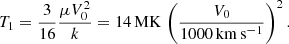 (9)
(9)
Here, V0 is the pre-shock velocity and μ is the mean atomic weight. With the radiative losses per volume equivalent to ϵ = nH2Λ(T), where nH is the hydrogen number density and Λ(T) is the cooling function, the characteristic time to radiate the thermal energy (cooling time) can be roughly estimated as
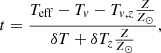
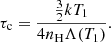 (10)
(10)
The factor of 4 in the denominator comes from the ratio of posts-shock and pre-shock densities at an infinitely large shock, ρ1/ρ0 = 4 (Feldmeier 2020). A large fraction of wind material is occupied by very hot gas in the case when the cooling time becomes comparable to the characteristic wind time, R*/v∞. With  , this gives a limiting mass-loss rate of
 (11)
(11)
For the calculation of the limiting mass-loss rate, we used the radiative losses from Schure et al. (2009), noting that they may be overestimated at around 105 K (Štofanová et al. 2021). For instance, for parameters corresponding to 10 Lac (Marcolino et al. 2017) R = 4 R⊙ and v∞ = 1200 km s−1, adopting V1 = v∞/2, we have T1 = 5 MK. For solar metallicity, this gives Λ(T1) = 2.7 × 10⁻²³ erg s−1 and a limiting mass-loss rate of 1.3 × 10⁻⁸ M⊙ yr−1. This value is not far from the lower limit of the 10 Lac mass-loss rate derived from infrared (IR) spectroscopy 3 × 10⁻⁸ M⊙ yr−1 (Law et al. 2024). For the SMC metallicity, Λ(T1) = 1.0 × 10⁻²³ erg s−1 and the limiting mass-loss rate is about 3 × 10⁻⁸ M⊙ yr−1 for the same terminal velocity.
For very low metallicities (Z < Z⊙/10) the cooling function becomes lower by a factor of about 2, shifting the limiting mass-loss rate to about 10−7 M⊙ yr−1. This implies that at the lowest metallicities considered here basically all O stars should be affected by weak-wind problem. The problem is less severe for B supergiants, which have slower winds and thus much weaker shocks and shorter shock cooling times.
5.4. Multicomponent effects
At very low metallicities, the coupling between radiatively accelerated heavy elements and light elements constituting the bulk of the wind, namely, hydrogen and helium, can become inefficient. This leads to frictional heating or decoupling of wind components (Springmann & Pauldrach 1992; Krtička & Kubát 2001; Owocki & Puls 2002). The importance of these effects can be estimated from the relative velocity difference between hydrogen and individual heavy elements.
We evaluated the relative velocity difference using Eq. (17) of Krtička (2006). For most of the models, the relative velocity difference is significantly lower than 1, meaning that the multicomponent effects are negligible. However, for several models with low mass-loss rates Ṁ ≲ 10−8 M⊙ yr−1 (especially in those with higher wind velocities), the difference becomes higher than one in the case of phosphorus in O stars and carbon, aluminium, and silicon in B stars. While the decoupling of phosphorus with low abundance would perhaps not significantly disrupt the flow, the decoupling of carbon can have more significant consequences.
However, the relative velocity difference reaches values of a few at most. Taking into account clumping, which is connected with higher densities in the region where the wind is accelerated, the real velocity differences are likely to be smaller. Thus, the effects of multicomponent structure are negligible in the studied sample.
6. Conclusions
We provide new line-driven wind models for luminous OB stars with metallicities down to 0.01 Z⊙. The models were calculated with our global wind code METUJE, which solves the hydrodynamical equations from nearly hydrostatic photosphere to supersonically expanding stellar wind. The radiative force accelerating the wind was derived from the solution of the radiative transfer equation in the comoving frame. The corresponding ionization and excitation structure was derived from the kinetic equilibrium equations (NLTE equations).
The models predict the wind structure including the wind mass-loss rate and terminal velocity just from the basic stellar parameters; namely, the stellar effective temperature, radius, mass, and chemical composition. The wind mass-loss rate depends mostly on the stellar luminosity and decreases with decreasing metallicity roughly as Ṁ ∼ Zα. For the metallicities down to the metallicity corresponding to the Magellanic Clouds (Z ≥ 0.2 Z⊙), the metallicity dependence of the mass-loss rate is rather weak, at α ≈ 0.6. For lower metallicities, this relationship steepens and α becomes higher than 1.
The wind mass-loss rate also significantly depends on the stellar effective temperature. The most significant feature coming from the temperature dependence of the wind mass-loss rate is the increase in the mass-loss rate with decreasing temperature for B supergiants with T < 20 kK, termed the bistability jump. This increase originates due to iron recombination and vanishes for subMagellanic metallicities (Z ≤ 0.1 Z⊙) coming from the weak iron contribution to the radiative force for very low metallicities.
Down to metallicities corresponding to the Magellanic Clouds, the predicted mass-loss rates agree reasonably well with observational estimates. On average, our mass-loss rates nicely reproduce the observational values with an exception of the SMC O stars. However, for the SMC metallicity our models reasonably reproduce the mass-loss rates in B supergiants, which other available predictions tend to either over- or underpredict to a significant degree. Moreover, the disagreement between observational mass-loss rate estimates and theoretical mass-loss rate predictions only concerns SMC O stars with low mass-loss rates. Therefore, the discrepancy is most likely caused by the inefficient shock cooling (weak-wind problem) and not by inadequate predictions.
For subMagellanic metallicities, both the theoretical mass-loss rate predictions and the observational values display significant scatter. On the theoretical side, the scatter is caused by a low number of lines significantly accelerating the wind, which leads to an increased sensitivity in the radiative acceleration to the detailed ionization structure of the wind. The observational values for low mass-loss rates Ṁ ≲ 10−7 M⊙ yr−1 and subMagellanic metallicities become affected by the inefficient shock cooling in the wind. The inefficient cooling leaves significant fraction of the stellar wind at very high temperatures weakening classical signatures of line-driven wind and the radiative force. Limiting the comparison only to stars with sufficiently high mass-loss rates, where the shock cooling is efficient, we arrive at good agreement between observational and theoretical mass-loss rate estimates.
The wind terminal velocity scales with the escape speed and with the stellar effective temperature. The predicted terminal velocities correspond well to the observational values up to the effective temperature of 30 kK. Above this value the models underpredict the observational values likely as a result of neglected wind clumping and X-ray emission. Despite this shortcoming, an extrapolation of terminal velocities derived below 30 kK to higher effective temperatures provides estimates that nicely agree with observations.
Here, we provide fits to theoretical predictions of the wind mass-loss rate and terminal velocity. The fits can be used in the evolutionary calculations and for the modeling of interaction of hot stars with their surrounding circumstellar environment.
Data availability
Wind model output files are available at the CDS via https://cdsarc.cds.unistra.fr/viz-bin/cat/J/A+A/702/A9
An exception is the C III 977 Å resonance line, which is able to significantly contribute to the line acceleration even in the B supergiant domain.
The code is available at https://zenodo.org/records/15965163
Acknowledgments
This work was supported by grant GA ČR 25-15910S. Computational resources were provided by the e-INFRA CZ project (ID:90254), supported by the Ministry of Education, Youth and Sports of the Czech Republic. The Astronomical Institute Ondřejov is supported by a project RVO:67985815 of the Academy of Sciences of the Czech Republic.
References
- Abbott, D. C. 1982, ApJ, 259, 282 [Google Scholar]
- Antokhin, I. I., Owocki, S. P., & Brown, J. C. 2004, ApJ, 611, 434 [Google Scholar]
- Asplund, M., Grevesse, N., Sauval, A. J., & Scott, P. 2009, ARA&A, 47, 481 [NASA ADS] [CrossRef] [Google Scholar]
- Babel, J. 1996, A&A, 309, 867 [Google Scholar]
- Backs, F., Brands, S. A., de Koter, A., et al. 2024, A&A, 692, A88 [NASA ADS] [CrossRef] [EDP Sciences] [Google Scholar]
- Bednarek, W. 2024, MNRAS, 527, 3818 [Google Scholar]
- Bernini-Peron, M., Marcolino, W. L. F., Sander, A. A. C., et al. 2023, A&A, 677, A50 [NASA ADS] [CrossRef] [EDP Sciences] [Google Scholar]
- Bernini-Peron, M., Sander, A. A. C., Ramachandran, V., et al. 2024, A&A, 692, A89 [NASA ADS] [CrossRef] [EDP Sciences] [Google Scholar]
- Bernini-Peron, M., Sander, A. A. C., Najarro, F., et al. 2025, A&A, 697, A41 [NASA ADS] [CrossRef] [EDP Sciences] [Google Scholar]
- Björklund, R., Sundqvist, J. O., Puls, J., & Najarro, F. 2021, A&A, 648, A36 [EDP Sciences] [Google Scholar]
- Björklund, R., Sundqvist, J. O., Singh, S. M., Puls, J., & Najarro, F. 2023, A&A, 676, A109 [NASA ADS] [CrossRef] [EDP Sciences] [Google Scholar]
- Bouret, J.-C., Lanz, T., Hillier, D. J., et al. 2003, ApJ, 595, 1182 [NASA ADS] [CrossRef] [Google Scholar]
- Bouret, J.-C., Hillier, D. J., Lanz, T., & Fullerton, A. W. 2012, A&A, 544, A67 [NASA ADS] [CrossRef] [EDP Sciences] [Google Scholar]
- Bouret, J.-C., Lanz, T., Martins, F., et al. 2013, A&A, 555, A1 [NASA ADS] [CrossRef] [EDP Sciences] [Google Scholar]
- Bouret, J.-C., Lanz, T., Hillier, D. J., et al. 2015, MNRAS, 449, 1545 [Google Scholar]
- Bouret, J. C., Martins, F., Hillier, D. J., et al. 2021, A&A, 647, A134 [NASA ADS] [CrossRef] [EDP Sciences] [Google Scholar]
- Brands, S. A., de Koter, A., Bestenlehner, J. M., et al. 2022, A&A, 663, A36 [Google Scholar]
- Brands, S. A., Backs, F., de Koter, A., et al. 2025, A&A, 697, A54 [NASA ADS] [CrossRef] [EDP Sciences] [Google Scholar]
- Carneiro, L. P., Puls, J., Sundqvist, J. O., & Hoffmann, T. L. 2016, A&A, 590, A88 [NASA ADS] [CrossRef] [EDP Sciences] [Google Scholar]
- Castor, J. I., Abbott, D. C., & Klein, R. I. 1975, ApJ, 195, 157 [Google Scholar]
- Cohen, D. H., Kuhn, M. A., Gagné, M., Jensen, E. L. N., & Miller, N. A. 2008, MNRAS, 386, 1855 [Google Scholar]
- Cohen, D. H., Wollman, E. E., Leutenegger, M. A., et al. 2014, MNRAS, 439, 908 [NASA ADS] [CrossRef] [Google Scholar]
- Crowther, P. A., Lennon, D. J., & Walborn, N. R. 2006, A&A, 446, 279 [NASA ADS] [CrossRef] [EDP Sciences] [Google Scholar]
- Feldmeier, A. 2020, Theoretical Fluid Dynamics (New York: Springer) [Google Scholar]
- Feldmeier, A., Puls, J., & Pauldrach, A. W. A. 1997, A&A, 322, 878 [NASA ADS] [Google Scholar]
- Furey, C., Telford, O. G., de Koter, A., et al. 2025, A&A, 698, A9 [NASA ADS] [CrossRef] [EDP Sciences] [Google Scholar]
- Garcia, M., Herrero, A., Najarro, F., Lennon, D. J., & Urbaneja, M. A. 2014, ApJ, 788, 64 [NASA ADS] [CrossRef] [Google Scholar]
- Gormaz-Matamala, A. C., Curé, M., Hillier, D. J., et al. 2021, ApJ, 920, 64 [NASA ADS] [CrossRef] [Google Scholar]
- Gormaz-Matamala, A. C., Curé, M., Meynet, G., et al. 2022, A&A, 665, A133 [NASA ADS] [CrossRef] [EDP Sciences] [Google Scholar]
- Gräfener, G., & Hamann, W.-R. 2005, A&A, 432, 633 [CrossRef] [EDP Sciences] [Google Scholar]
- Gräfener, G., & Hamann, W.-R. 2008, A&A, 482, 945 [NASA ADS] [CrossRef] [EDP Sciences] [Google Scholar]
- Gvaramadze, V. V., Alexashov, D. B., Katushkina, O. A., & Kniazev, A. Y. 2018, MNRAS, 474, 4421 [Google Scholar]
- Hawcroft, C., Sana, H., Mahy, L., et al. 2021, A&A, 655, A67 [NASA ADS] [CrossRef] [EDP Sciences] [Google Scholar]
- Hawcroft, C., Mahy, L., Sana, H., et al. 2024a, A&A, 690, A126 [NASA ADS] [CrossRef] [EDP Sciences] [Google Scholar]
- Hawcroft, C., Sana, H., Mahy, L., et al. 2024b, A&A, 688, A105 [NASA ADS] [CrossRef] [EDP Sciences] [Google Scholar]
- Hillier, D. J., & Miller, D. L. 1999, ApJ, 519, 354 [Google Scholar]
- Hubeny, I., & Mihalas, D. 2014, Theory of Stellar Atmospheres (Princeton: Princeton University Press) [Google Scholar]
- Kaaret, P., Ward, M. J., & Zezas, A. 2004, MNRAS, 351, L83 [NASA ADS] [CrossRef] [Google Scholar]
- Keszthelyi, Z., Puls, J., & Wade, G. A. 2017, A&A, 598, A4 [NASA ADS] [CrossRef] [EDP Sciences] [Google Scholar]
- Kobulnicky, H. A., Chick, W. T., & Povich, M. S. 2019, AJ, 158, 73 [NASA ADS] [CrossRef] [Google Scholar]
- Krtička, J. 2006, MNRAS, 367, 1282 [NASA ADS] [CrossRef] [Google Scholar]
- Krtička, J., & Kubát, J. 2001, A&A, 377, 175 [NASA ADS] [CrossRef] [EDP Sciences] [Google Scholar]
- Krtička, J., & Kubát, J. 2009a, A&A, 493, 585 [NASA ADS] [CrossRef] [EDP Sciences] [Google Scholar]
- Krtička, J., & Kubát, J. 2009b, MNRAS, 394, 2065 [Google Scholar]
- Krtička, J., & Kubát, J. 2010, A&A, 519, A50 [NASA ADS] [CrossRef] [EDP Sciences] [Google Scholar]
- Krtička, J., & Kubát, J. 2014, A&A, 567, A63 [NASA ADS] [CrossRef] [EDP Sciences] [Google Scholar]
- Krtička, J., & Kubát, J. 2017, A&A, 606, A31 [NASA ADS] [CrossRef] [EDP Sciences] [Google Scholar]
- Krtička, J., & Kubát, J. 2018, A&A, 612, A20 [NASA ADS] [CrossRef] [EDP Sciences] [Google Scholar]
- Krtička, J., Kubát, J., & Krtičková, I. 2018, A&A, 620, A150 [NASA ADS] [CrossRef] [EDP Sciences] [Google Scholar]
- Krtička, J., Kubát, J., & Krtičková, I. 2020, A&A, 635, A173 [NASA ADS] [CrossRef] [EDP Sciences] [Google Scholar]
- Krtička, J., Kubát, J., & Krtičková, I. 2021, A&A, 647, A28 [NASA ADS] [CrossRef] [EDP Sciences] [Google Scholar]
- Krtička, J., Kubát, J., & Krtičková, I. 2024, A&A, 681, A29 [NASA ADS] [CrossRef] [EDP Sciences] [Google Scholar]
- Kudritzki, R.-P., & Puls, J. 2000, ARA&A, 38, 613 [Google Scholar]
- Lagae, C., Driessen, F. A., Hennicker, L., Kee, N. D., & Sundqvist, J. O. 2021, A&A, 648, A94 [NASA ADS] [CrossRef] [EDP Sciences] [Google Scholar]
- Lamers, H. J. G. L. M., Snow, T. P., & Lindholm, D. M. 1995, ApJ, 455, 269 [Google Scholar]
- Lanz, T., & Hubeny, I. 2003, ApJS, 146, 417 [NASA ADS] [CrossRef] [Google Scholar]
- Lanz, T., & Hubeny, I. 2007, ApJS, 169, 83 [CrossRef] [Google Scholar]
- Law, D. R., Hawcroft, C., Smith, L. J., et al. 2024, ApJ, 976, L25 [Google Scholar]
- Marcolino, W. L. F., Bouret, J.-C., Martins, F., et al. 2009, A&A, 498, 837 [NASA ADS] [CrossRef] [EDP Sciences] [Google Scholar]
- Marcolino, W. L. F., Bouret, J. C., Lanz, T., Maia, D. S., & Audard, M. 2017, MNRAS, 470, 2710 [NASA ADS] [CrossRef] [Google Scholar]
- Marcolino, W. L. F., Bouret, J. C., Rocha-Pinto, H. J., Bernini-Peron, M., & Vink, J. S. 2022, MNRAS, 511, 5104 [NASA ADS] [CrossRef] [Google Scholar]
- Martins, F., Schaerer, D., & Hillier, D. J. 2005, A&A, 436, 1049 [NASA ADS] [CrossRef] [EDP Sciences] [Google Scholar]
- Martins, F., Schaerer, D., Hillier, D. J., & Heydari-Malayeri, M. 2004, A&A, 420, 1087 [NASA ADS] [CrossRef] [EDP Sciences] [Google Scholar]
- Michaud, G., Richer, J., & Vick, M. 2011, A&A, 534, A18 [NASA ADS] [CrossRef] [EDP Sciences] [Google Scholar]
- Mihalas, D., Kunasz, P. B., & Hummer, D. G. 1975, ApJ, 202, 465 [CrossRef] [Google Scholar]
- Müller, P. E., & Vink, J. S. 2008, A&A, 492, 493 [NASA ADS] [CrossRef] [EDP Sciences] [Google Scholar]
- Najarro, F., Hanson, M. M., & Puls, J. 2011, A&A, 535, A32 [NASA ADS] [CrossRef] [EDP Sciences] [Google Scholar]
- Owocki, S. P., & Puls, J. 2002, ApJ, 568, 965 [NASA ADS] [CrossRef] [Google Scholar]
- Owocki, S. P., Castor, J. I., & Rybicki, G. B. 1988, ApJ, 335, 914 [NASA ADS] [CrossRef] [Google Scholar]
- Pauldrach, A., Puls, J., & Kudritzki, R. P. 1986, A&A, 164, 86 [NASA ADS] [Google Scholar]
- Pauldrach, A. W. A., & Puls, J. 1990, A&A, 237, 409 [NASA ADS] [Google Scholar]
- Peron, G., Casanova, S., Gabici, S., Baghmanyan, V., & Aharonian, F. 2024, Nat. Astron., 8, 530 [CrossRef] [Google Scholar]
- Petrov, B., Vink, J. S., & Gräfener, G. 2014, A&A, 565, A62 [NASA ADS] [CrossRef] [EDP Sciences] [Google Scholar]
- Petrov, B., Vink, J. S., & Gräfener, G. 2016, MNRAS, 458, 1999 [NASA ADS] [CrossRef] [Google Scholar]
- Prinja, R. K., Barlow, M. J., & Howarth, I. D. 1990, ApJ, 361, 607 [NASA ADS] [CrossRef] [Google Scholar]
- Puls, J., Springmann, U., & Lennon, M. 2000, A&AS, 141, 23 [NASA ADS] [CrossRef] [EDP Sciences] [Google Scholar]
- Renzo, M., Ott, C. D., Shore, S. N., & de Mink, S. E. 2017, A&A, 603, A118 [NASA ADS] [CrossRef] [EDP Sciences] [Google Scholar]
- Reyero Serantes, S., Oskinova, L., Hamann, W. R., et al. 2024, A&A, 690, A347 [NASA ADS] [CrossRef] [EDP Sciences] [Google Scholar]
- Roman-Duval, J., Fischer, W. J., Fullerton, A. W., et al. 2025, ApJ, 985, 109 [Google Scholar]
- Sander, A. A. C., & Vink, J. S. 2020, MNRAS, 499, 873 [Google Scholar]
- Schure, K. M., Kosenko, D., Kaastra, J. S., Keppens, R., & Vink, J. 2009, A&A, 508, 751 [NASA ADS] [CrossRef] [EDP Sciences] [Google Scholar]
- Springmann, U. W. E., & Pauldrach, A. W. A. 1992, A&A, 262, 515 [NASA ADS] [Google Scholar]
- Stift, M. J., & Alecian, G. 2012, MNRAS, 425, 2715 [Google Scholar]
- Sundqvist, J. O., Björklund, R., Puls, J., & Najarro, F. 2019, A&A, 632, A126 [NASA ADS] [CrossRef] [EDP Sciences] [Google Scholar]
- Szécsi, D., & Wünsch, R. 2019, ApJ, 871, 20 [CrossRef] [Google Scholar]
- Štofanová, L., Kaastra, J., Mehdipour, M., & de Plaa, J. 2021, A&A, 655, A2 [NASA ADS] [CrossRef] [EDP Sciences] [Google Scholar]
- Šurlan, B., Hamann, W.-R., Aret, A., et al. 2013, A&A, 559, A130 [NASA ADS] [CrossRef] [EDP Sciences] [Google Scholar]
- Telford, O. G., Chisholm, J., Sander, A. A. C., et al. 2024, ApJ, 974, 85 [NASA ADS] [Google Scholar]
- Tramper, F., Sana, H., de Koter, A., Kaper, L., & Ramírez-Agudelo, O. H. 2014, A&A, 572, A36 [NASA ADS] [CrossRef] [EDP Sciences] [Google Scholar]
- Verhamme, O., Sundqvist, J., de Koter, A., et al. 2024, A&A, 692, A91 [NASA ADS] [CrossRef] [EDP Sciences] [Google Scholar]
- Vink, J. S. 2018, A&A, 619, A54 [NASA ADS] [CrossRef] [EDP Sciences] [Google Scholar]
- Vink, J. S. 2022, ARA&A, 60, 203 [NASA ADS] [CrossRef] [Google Scholar]
- Vink, J. S., de Koter, A., & Lamers, H. J. G. L. M. 1999, A&A, 350, 181 [Google Scholar]
- Vink, J. S., de Koter, A., & Lamers, H. J. G. L. M. 2001, A&A, 369, 574 [NASA ADS] [CrossRef] [EDP Sciences] [Google Scholar]
- Vink, J. S., Mehner, A., Crowther, P. A., et al. 2023, A&A, 675, A154 [NASA ADS] [CrossRef] [EDP Sciences] [Google Scholar]
All Tables
Predicted terminal velocities v∞ (in km s−1) and the mass-loss rates Ṁ (in M⊙ yr−1) for B supergiants.
Predicted terminal velocities v∞ (in km s−1) and the mass-loss rates Ṁ (in M⊙ yr−1) for O stars.
All Figures
|
Fig. 1. Wind mass-loss rate as a function of the stellar luminosity from METUJE models at different metallicities for stars with Teff ≥ 27.5 kK. |
| In the text | |
|
Fig. 2. Power of the metallicity dependence of the mass-loss rate Ṁ ∼ Zα (Eq. (1)) plotted as a function of the stellar effective temperature for models at different metallicities. Dashed lines describe mean relationship derived for individual metallicities. |
| In the text | |
|
Fig. 3. Relative contribution of selected elements to the line radiative force as a function of the effective temperature, plotted at the wind critical point for O giants and B supergiants with M = 40 M⊙. While line colors denote individual elements, line styles differentiate between metallicity, with the solid line corresponding to Z⊙, dashed line to 0.1 Z⊙, and dotted line to 0.01 Z⊙. The thick blue line gives the mean ionization state driving the wind for 0.1 Z⊙. The mean ionization state is defined as ∑fizi/(∑fi), where fi is the contribution of ion i (with charge zi) to the line radiative force. The corresponding axis is on the right. The values of the radiative force were obtained within the Sobolev approximation. |
| In the text | |
|
Fig. 4. Relative contribution of three lines that drive the wind most strongly to the radiative force. Plotted as a function of the stellar effective temperature for different metallicities at the critical point using the Sobolev approximation for O giants and 40 M⊙ B supergiants. We labeled selected strongest lines with wavelength in Å. |
| In the text | |
|
Fig. 5. Mass-loss rate variations with the temperature for B supergiants. The line color denotes metallicity, while the dash type corresponds to different stellar luminosities (log(L/L⊙) = 5.28, 5.66, and 5.88). |
| In the text | |
|
Fig. 6. Predicted ratio of the wind terminal velocity, v∞, and escape speed, vesc, as a function of the effective temperature. Solid lines colored according to the metallicity give fit to theoretical predictions (see Eq. (4)). |
| In the text | |
|
Fig. 7. Predicted wind terminal velocity as a function of the effective temperature for different metallicities. The linear fits are colored according to metallicity and derived from Eq. (7). |
| In the text | |
|
Fig. 8. Ratio of the predicted mass-loss rates and their observational estimates plotted as a function of the stellar effective temperature for stars from our Galaxy. The theoretical mass-loss rates from Vink et al. (2001), Björklund et al. (2023), and this paper are compared with observational estimates of Najarro et al. (2011), Bouret et al. (2012), Šurlan et al. (2013), Marcolino et al. (2017, supergiants), Hawcroft et al. (2021), and Bernini-Peron et al. (2023). The horizontal lines give mean values for individual theoretical predictions. |
| In the text | |
|
Fig. 9. Ratio of the predicted mass-loss rates and their observational estimates plotted as a function of the effective temperature for stars from the LMC. The theoretical mass-loss rates from Vink et al. (2001), Björklund et al. (2023), and this paper are compared with observational estimates of Brands et al. (2022), Hawcroft et al. (2024a), and Verhamme et al. (2024). The horizontal lines give mean values for individual theoretical predictions. |
| In the text | |
|
Fig. 10. Ratio of the predicted mass-loss rates and their observational estimates plotted as a function of the effective temperature for stars from the SMC. The theoretical mass-loss rates from Vink et al. (2001), Björklund et al. (2023), and this paper are compared with observational estimates of Bouret et al. (2013, 2021), Backs et al. (2024), and Bernini-Peron et al. (2024). The horizontal lines give mean values for individual theoretical predictions. |
| In the text | |
|
Fig. 11. Ratio of the predicted mass-loss rates and their observational estimates plotted as a function of the effective temperature for stars from galaxies with subMagellanic metallicities. Pink box denotes the only three stars with clumping-corrected mass-loss rate Ṁ > 10−7 M⊙ yr−1. |
| In the text | |
|
Fig. 12. Observational values of the wind terminal velocities (Crowther et al. 2006; Hawcroft et al. 2024b) compared with theoretical predictions Eq. (7) for stars from the Galaxy, LMC, and SMC. |
| In the text | |
|
Fig. 13. Observational values of the wind terminal velocities (Bouret et al. 2015; Telford et al. 2024; Furey et al. 2025) compared with theoretical values for stars with subMagellanic metallicities. |
| In the text | |
Current usage metrics show cumulative count of Article Views (full-text article views including HTML views, PDF and ePub downloads, according to the available data) and Abstracts Views on Vision4Press platform.
Data correspond to usage on the plateform after 2015. The current usage metrics is available 48-96 hours after online publication and is updated daily on week days.
Initial download of the metrics may take a while.